Frequentist and Bayesian Analysis of Random Coefficient Autoregressive models

Abstract

WANG, DAZHE. Frequentist and Bayesian Analysis of Random Coefficient Autore-gressive Models. (Under the direction of Dr. Sastry G. Pantula and Dr. Sujit K. Ghosh.)

Random Coefficient Autoregressive (RCA) models are obtained by introducing random coefficients to an AR or more generally ARMA model. These models have second order properties similar to that of ARCH and GARCH models. Historically an RCA model has been used to model the conditional mean of a time series, but it can also be viewed as a volatility model. In this thesis, we consider both Frequentist and Bayesian approaches to analyze the first order RCA models. For a weakly sta-tionary RCA(1), it has been shown that the Maximum Likelihood Estimates (MLEs) are strongly consistent and satisfy a classical Central Limit Theorem. We consider a broader class of RCA(1) models whose parameters lie in the region of strict station-arity and ergodicity. We show that similar asymptotic properties can be extended to this class of models which includes the unit-root RCA(1) as a special case. The existence of a unit root in an RCA(1) has significant impact on the inference of data especially in the aspect of model forecasting. We develop the Wald criterion based on MLEs for testing unit root and evaluate its power via simulation studies.

FREQUENTIST AND BAYESIAN ANALYSIS OF RANDOM COEFFICIENT AUTOREGRESSIVE MODELS

by

DAZHE WANG

A dissertation submitted to the Graduate Faculty of North Carolina State University

in partial fulfillment of the requirements for the Degree of

Doctor of Philosophy

STATISTICS

Raleigh

2003

APPROVED BY:

Dr. Sastry G. Pantula Dr. Sujit K. Ghosh

CO-Chair of Advisory Committee CO-Chair of Advisory Committee

Biography

Acknowledgements

I would first like to thank my co-advisors, Dr. Pantula and Dr. Ghosh for their guidance, advice and support throughout my research work. I am also grateful to my committee members, Dr. Dickey and Dr. Gumpertz for their valuable suggestions and comments on the revision of the thesis.

I owe thanks to the following people (past and present) in the Statistics De-partment of NC State University: Dr. Bibhuti B. Bhattacharyya, Terry Byron, Dr. Dennis D. Boos, Dr. Peter Bloomfield, Janice Gaddy, Dr. Subhashis Ghosal, Dr. Palanikumar Ravindran and Dr. Zeynep Isil Kalaylioglu.

Special thanks to my colleagues in Statistical Sciences group of GlaxoSmithKline in Research Triangle Park - thank you for giving me the opportunity to work closely with you and learn from you.

I couldn’t have accomplished this thesis and this degree without the support from my family. I want to take this time to thank my loving parents and my brother Yingzhe, for their support, understanding and encouragement in my pursuit of this degree and to all of my other endeavors in life.

Contents

List of Figures viii

List of Tables x

1 Random Coefficient Autoregressive (RCA) models 1

1.1 Introduction . . . 1

1.2 Parameter estimation in RCA(1) models . . . 6

1.3 Motivation for unit-root testing in RCA(1) . . . 14

2 Frequentist approach to RCA(1) models 19 2.1 Introduction . . . 19

2.2 Strict stationarity and ergodicity of RCA(1) . . . 21

2.3 Maximum likelihood method . . . 24

2.3.1 The computation of Maximum Likelihood Estimates . . . 27

2.3.2 The strong consistency of Maximum Likelihood Estimates . . 30

2.3.3 The Central Limit Theorem . . . 35

2.3.5 Unit-root testing for RCA(1) based on MLEs . . . 49

2.4 A simulation study . . . 51

3 Bayesian approach to RCA(1) models 67 3.1 Introduction . . . 67

3.2 Bayesian estimation for RCA(1) . . . 70

3.2.1 Choice of prior densities . . . 70

3.2.2 Model selection . . . 71

3.2.3 Posterior inference via Gibbs Sampling . . . 73

3.2.4 A simulation study . . . 78

3.3 Bayesian unit-root testing for RCA(1) . . . 86

3.3.1 Choice of prior densities . . . 88

3.3.2 Gibbs Sampling algorithm . . . 90

3.3.3 Bayesian unit-root testing procedures . . . 92

3.3.4 A simulation study . . . 96

4 Application 106 4.1 NASDAQ stock index data . . . 106

4.1.1 Parameter estimation . . . 107

4.1.2 Model selection . . . 109

4.1.3 Unit-root testing . . . 110

4.1.4 Forecasting . . . 111

4.2.1 Parameter estimation . . . 113 4.2.2 Unit-root testing . . . 115 4.2.3 Forecasting . . . 116

5 Conclusions 120

List of Figures

1.1 Plot of the returns xt versus time t simulated from several RCA(1) models (n=500 observations) . . . 7 1.2 Comparison of sample path for RCA(1) series with η < 1 and η = 1

(n=500 observations) . . . 16

2.1 Region of strict stationarity and ergodicity for RCA(1) . . . 25 2.2 Histogram of Tw for different unit-root RCA(1) models (sample size

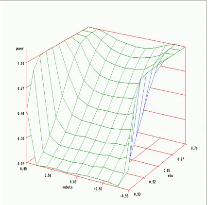
n=5000, 1000 MC replications) . . . 59 2.3 Power of Wald test on the space of (µβ, η) (sample size n=500, 1000

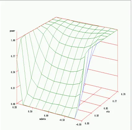
MC replications) . . . 60 2.4 Power of Wald test on the space of (µβ, η) (sample size n=1000, 1000

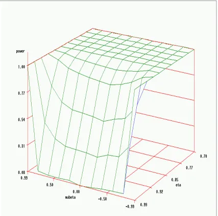
MC replications) . . . 61 2.5 Power of Wald test on the space of (µβ, η) (sample size n=5000, 1000

MC replications) . . . 62 2.6 Power of Wald test as a function ofµβ for various fixed values ofη≥µ2β

2.7 Power of Wald test as a function ofµβ for various fixed values ofη≥µ2β (sample size n=1000, 1000 MC replications) . . . 64 2.8 Power of Wald test as a function ofµβ for various fixed values ofη≥µ2β

(sample size n=5000, 1000 MC replications) . . . 65

4.1 Time series plot of the NASDAQ daily transaction volume data (vol-ume in log scale) . . . 107 4.2 Time series plot of the residuals after detrending for NASDAQ data 108 4.3 Forecasts for detreneded NASDAQ daily transaction volume data based

on RCA(1) and AR(1)-GARCH(1,2) models . . . 113 4.4 Forecasts for NASDAQ daily transaction volume data based on RCA(1)

model . . . 114 4.5 Time series plot of the IBM daily transaction volume data (volume in

million) . . . 115 4.6 Forecasts for IBM daily transaction volume data . . . 117 4.7 Time series plot for detrended IBM daily transaction volume data

(vol-ume in log scale) . . . 118 4.8 Forecasts for IBM daily transaction volume data based on fitting an

List of Tables

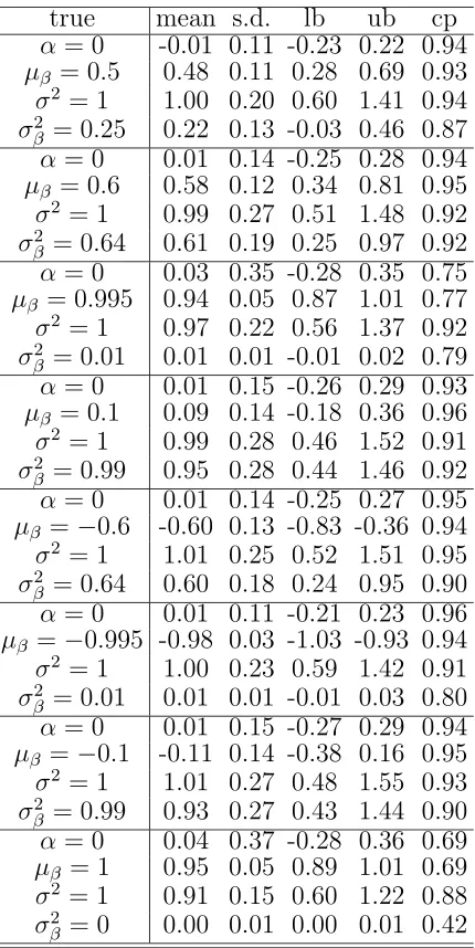
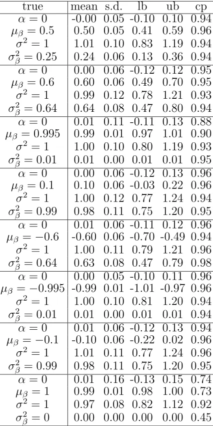
2.1 Monte Carlo average of MLEs for different RCA(1) models (sample size n=100, 500 MC replications). . . 56 2.2 Monte Carlo average of MLEs for different RCA(1) models (sample

size n=500, 500 MC replications). . . 57 2.3 Empirical significance levels and powers from the 5% level Wald test

for different sample sizes (500 MC replications) . . . 66 2.4 Average proportion that the MLEs for RCA(1) models fall outside

the strictly stationary and ergodic region (sample size n=500, 500 MC replications) . . . 66

3.1 Monte Carlo average of posterior summaries for different RCA(1) mod-els (sample size n=100, 500 MC replications). . . 81 3.2 Monte Carlo average of posterior summaries for different RCA(1)

mod-els (sample size n=500, 500 MC replications). . . 82 3.3 Monte Carlo average of AIC and GGC for different RCA(1) models

3.4 Monte Carlo average of AIC and GGC for different RCA(1) models (sample size n=500, 500 MC replications). . . 84 3.5 Posterior summary for fitting RCA(1) and AR(1) when data are

gener-ated from RCA(1) and AR(1) (sample size n=100, 500 MC replications). 87 3.6 Posterior summary for fitting RCA(1) and AR(1) when data are

gener-ated from RCA(1) and AR(1) (sample size n=500, 500 MC replications). 87 3.7 Average values of Posterior Odds (PO) and Bayes Factor (BF) and the

Proportion of Correct Decision (PCD) for unit-root testing (sample size n=300, 100 MC replications). . . 102 3.8 Proportion of Correct Decision (PCD) for unit-root testing based on

BF method using MU(0.5) for different sample sizes (500 MC replica-tions). . . 103 3.9 Proportion of Correct Decision (PCD) for unit-root testing based on

PI method (sample size n=1500, 100 MC replications). . . 104 3.10 Proportion of Correct Decision (PCD) for unit-root testing based on PI

method using Uinf(0,2) for different sample sizes (500 MC replications). 105 3.11 Proportion of Correct Decision (PCD) for unit-root testing based on PI

method using MU(0.5) for different sample sizes (500 MC replications). 105

4.1 MLEs of an RCA(1) fit to NASDAQ daily transaction volume data . 109 4.2 Bayesian posterior summaries of an RCA(1) fit to NASDAQ daily

4.3 AIC from fitting different volatility models to NASDAQ daily transac-tion volume data . . . 110 4.4 Frequentist and Bayesian unit-root tests for NASDAQ daily

transac-tion volume data . . . 111 4.5 MLEs of an RCA(1) fit to IBM daily transaction volume data . . . . 114 4.6 Bayesian posterior summaries of an RCA(1) fit to IBM daily

transac-tion volume data . . . 115 4.7 Frequentist and Bayesian unit-root tests for IBM daily transaction

vol-ume data . . . 116

5.1 Coverage probabilities of Frequentist and Bayesian estimation for dif-ferent RCA(1) models (sample size n=100, 500 MC replications). . . 124 5.2 Total error rates of Frequentist and Bayesian unit-root tests (sample

size n=1000, 500 MC replications). . . 125 5.3 Total error rates of Frequentist and Bayesian unit-root tests (sample

size n=2500, 500 MC replications). . . 125 5.4 Total error rates of Frequentist and Bayesian unit-root tests (sample

Chapter 1

Random Coefficient Autoregressive

(RCA) models

1.1

Introduction

variance of xt given the past information, that is,

µt = E(xt|Ft−1)

σ_t2 = V ar(xt|Ft−1) (1.1)

where Ft−1 denotes the information set available up to time t−1. Empirically, the conditional mean µt has simple structure, and it is usually assumed that xt follows a simple time series model such as a stationary ARMA(p,q) model, see Tsay (2002) for some examples. Modeling the conditional variance is usually classified into two general categories in the literature: one is to use a deterministic function that governs the evolution of σ_t2, whereas the other models σ2_t through a stochastic relation. The GARCH type of model belongs to the first category, and the Stochastic Volatility model falls in the second category.

A model that is commonly used to describe the unobserved volatility is known as Autoregressive Conditional Heteroscedastic (ARCH) model first proposed by Engle (1982). The most simple ARCH model, denoted by ARCH(1), is defined via the mean-corrected return, or the shock,rt =xt−µt as,

rt = σtut

σ_t2 = α₀+α₁r_t2₋₁. (1.2)

rt−1 and hence a large past square return value implies a large conditional variance σ_t2. Consequently, rt tends to assume a large value in absolute scale. This means that under ARCH structure, a large shock is often followed by another large shock. This feature is similar to the volatility clustering observed commonly in asset return series.

Empirically, an ARCH model often requires many parameters to adequately de-scribe the volatility process of an asset return. An extension to ARCH proposed by Bollerslev (1986) is known as Generalized ARCH (GARCH) model. The idea of GARCH model is that the volatility is allowed to depend not only on the past return, but also on the past volatility. For example, GARCH(1,1) is expressed as,

rt = σtut

σ_t2 = α₀ +α₁r_t2₋₁+β₁σ2_t−1, (1.3) whereα₀ >0,α₁ ≤1, β₁ ≥0 andα₁+β₁ <1. Similar to an ARCH model, a GARCH model can pick up the volatility clustering feature in real financial time series.

Another way to produce conditional heteroscedasticity is to use so-called Con-ditional Heteroscedastic ARMA (CHARMA) model, see Tsay (1987). A CHARMA model is different from an ARCH model but these two models possess similar second-order properties. A pth _{order CHARMA is defined as,}

{_δ˜_{t} ={(δ1t, . . . , δpt)} is a sequence of iid random vectors with mean zero and}

non-negative definite covariance matrix Ω, and {δ˜t} is independent of {ηt}. It should be noted that the CHARMA model uses cross-products of the lagged return of rt in the volatility equation, while the ARCH model doesn’t. However, if the matrix Ω in CHARMA is diagonal, then these two models have the same conditional variance structure.

Another class of models that are very similar in spirit to CHARMA models is known as the Random Coefficient Autoregressive (RCA) models studied in detail by Nicholls and Quinn (1982). Historically an RCA model has been used to model conditional mean of a time series, but it can also be viewed as a volatility model. A return series {xt} is said to follow an RCA model of order p if it satisfies,

xt = α+ p

j=1

βtjxt−j +t. (1.5)

where ˜βt = (βt₁, . . . , βtp), is a sequence of independent random vectors with mean ˜

µβ = (µβ1, . . . , µβp) and covariance matrix Ωβ. Furthermore ˜βt andtare assumed to be independent. The conditional mean and conditional variance of RCA model have the same form as that of the CHARMA model. However, there is a subtle difference between these two models in modeling financial time series data. For RCA models, the volatility is a quadratic function of the observed lagged returns xt’s, whereas for CHARMA models, the volatility is a quadratic function of the lagged mean-corrected returns rt’s.

are satisfied:

1. E(rt) = 0 for any t >0;

2. E(rtrt+h) = 0 for any t >0 and h >0;

3. E[g(rt)g(rt+h)]= 0, where g(.) is an even function.

In another word, the series {rt} is uncorrelated but dependent. Consider an RCA series, in particular, a first order RCA series {xt},

xt =α+βtxt−1+t=α+µβxt−1+rt,

where rt =σβvtxt−1+t, where vt is a random variable with mean 0 and variance 1 and independent of t. It is obvious that {rt} series satisfy the first two properties described above. For the third property, it can be shown that for g(r) = r2 or g(r) = |r|, the property holds. This justifies that we can use an RCA model as a volatility model.

In this thesis, we will consider only the simplified case of RCA model, namely the case with p= 1. With a slight abuse of notation, we will write the model (1.5) as,

xt = α+βt1xt−1+t. (1.6)

of problem at hand might motivate to assume the two random variables βt and t to be correlated, see Hwang and Basawa (1998). Another modification might be to drop the intercept term α from the model, see Nicholls and Quinn (1982).

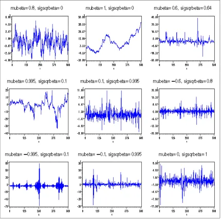
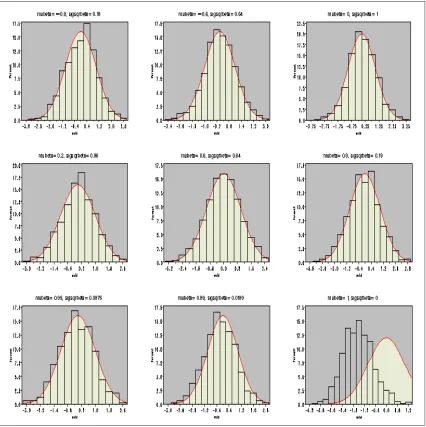
In Figure (1.1), we present several simulated RCA(1) series of lengthn = 500. To generate the RCA series for these plots we have fixed α = 0 and σ2 = 1 and used different values for the pair (µβ, σβ2).See the top of each plot to find the specific values of the pair (µβ, σβ2) that generated different series. It turns out that the RCA series is stationary if µ2_β +σ_β2 <1. It is also obvious that when σ2_β = 0 the RCA becomes a regular AR series. These time series plots in Figure (1.1) clearly demonstrate the flexibility of the RCA models in representing different types of volatility models. One feature observed from these plots is the clustering of the volatility. For instance, for the case with µβ = −0.995 and σβ2 = 0.1, we see that the volatility is high and clustered around time t= 250 and t= 400, and low for other time period.

1.2

Parameter estimation in RCA(1) models

Figure 1.1: Plot of the returnsxtversus timetsimulated from several RCA(1) models (n=500 observations)

from the model. For RCA(1) model, they write

whereβt’s are iid random variables with meanµβ and varianceσβ2,t’s are iid random variables with mean 0 and variance σ2, and βt’s and t’s are independent.

The first estimation method they propose is based on the least square criterion, which is a two-step procedure. Let Ft be the information set up to time t, and let ut=xt−µβxt−1, then it is seen that

E(ut|Ft−1) = 0 and E(u2t|Ft−1) = σ2+σβ2x2t−1

Given a sample x₀, x₁, . . . , xn, the first step is to estimateµβ by minimizing n

t=1u2t with respect to µβ, thus the least square estimate ˆµβ,LS is given by,

ˆ µβ,LS =

_n

t₌₁ x2_t−1

−1n

t₌₁

xt−1xt.

The second step in the estimation procedure is to form the residual ˆut=xt−µˆβ,LSxt−1 and then regress ˆu2_t on 1 and x2_t−1, which is equivalent to minimize n_t=1(ˆu2_t −σ2− σ_β2x2_t−1)2 with respect toσ2 and σ2_β. Consequently the LS estimates of σ2 and σ_β2 are obtained as,

ˆ σ_β,LS2 =

_n

t=1

(x2_t−1−z)¯ 2

_{−1 n}

t=1 ˆ

u2_t(x2_t−1−z)¯ and

ˆ

σ2_LS =n−1 n

t=1 ˆ

u2_t −σˆ_β,LS2 z,¯

where ¯z = n−1n_t=1x2_t−1. It is shown that if the second moments of βt and t exist, then ˆµβ,LS is a consistent estimator for µβ. And if E(x4t)< ∞ then

√

n(ˆµβ,LS−µβ) converges in distribution to a normal random variable. For Model (1.7), let us define ˆ

(µβ, σ2β, σ2). And

√

n(ˆθLS−θ) converges to a normal random variable ifE(x8t)<∞. In practice, the eighth moment condition required for xt is rather restrictive and not easy to verify. However, if βt and t are assumed to be jointly normal, then a necessary and sufficient condition for E(x4_t) < ∞ becomes µ4_β + 6µ2_βσ2_β + 3σ_β2 < 1. Under this condition, the LS estimator ˆθLS converges almost surely to θ and hence proves to be a good initial estimate for θ in any iterative estimation procedure such as the Maximum Likelihood procedure that will be discussed momentarily.

The second estimation procedure Nicholls and Quinn studied in great details is based on the maximum likelihood criterion. Because of the non-linear nature of the RCA model, the maximum likelihood type of estimation method would be an iterative procedure. It is desirable to commence the procedure at some point close to the global maximum of the likelihood function. The least square estimators, if consistent, prove to be a good initial choice for this iterative procedure. The maximum likelihood procedure is based on maximizing the likelihood function constructed by assuming that βt and t are jointly normal. The estimates obtained this way are referred to as the Maximum Likelihood estimates, or MLE, and denoted by ˆθM LE. Nicholls and Quinn show that under the normality of βt and t, if the process is second order stationary, then ˆθM LE is consistent for θ and moreover, if the fourth moments of βt and t are finite, then

√

n(ˆθM LE −θ) has a limiting normal distribution.

There are other approaches in the literature which is related to the estimation of the parameter µβ in the RCA(1) model (1.7).

indexed by a family of bounded measurable functions. Let Φ be the set of all bounded measurable function φ such thatxφ(x)>0 for x= 0. Set

ˆ

µn(φ) = n

j=1φ(xj−1)xj n

j=1φ(xj−1)xj−1

and V(φ) = E[φ

2_(x

0)w(x0)]

[E(φ(x₀)x₀)]2

wherew(x) =σ2+σ2_βx2. It is shown that for every φ∈Φ,√n(ˆµn(φ)−µβ) converges in distribution to a normal random variable with mean 0 and variance V(φ). Fur-thermore, an asymptotically optimal estimator which possesses the smallest variance within this class of estimators is defined by taking

φ(x) = φ(x) = x

1 +τ x2, where τ = σ2_β σ2. Hence, Schick’s estimator has the form,

ˆ

µn(φ) = _n

t=1

xtxt−1 σ2+σ2_βx2_t−1

n

t=1

x2_t−1 σ2+σ_β2x2_t−1

₋₁

(1.8)

In practice,τ is an unknown quantity in the above expression. Schick provides a class of consistent estimates τn, for τ and shows that by replacing τ by τn in ˆµn(φ), the asymptotic normality still holds, that is,

√

n(ˆµn(φτˆn)−µβ) D

−→N[0, V(φτ)].

Thavaneswaran and Abraham (1998) consider the RCA models as a special case of the general non-linear time series and discuss the estimation problem using the esti-mation equation approach of Godambe (1985). Godambe’s idea is to consider the so-called regular unbiased estimation function, that is, a real function g ofx₀, x₁, . . . , xn and the parameter θ such that

EF[g(x0, x1, . . . , xn;θ(F)] = 0 forF ∈ F,

where F is the class of distribution functions F on Rn+1_{. Let F}

t be the σ-field generated byx₀, x₁, . . . , xtand letLbe the class of estimating functionsg of the form g = n_t=1htat−1, where the function ht is such that E(ht|Ft−1) = 0 and at−1 is a function of x₀, x₁, . . . , xt−1 and θ. Godambe’s Theorem states that in the class L of unbiased estimating functions g, the optimum estimation functiong _{is the one which} minimizes EF(g2)/EF(∂g_∂θ)2 for all F ∈ F and is given by

g = n

t=0

htat−1, where at−1 =E(∂ht/∂θ|Ft−1)/E(h2t|Ft−1).

For RCA(1) model (1.7), by taking g = n_t=1htat−1, where ht = xt−E(xt|Ft−1) = xt−µβxt−1, as the estimating function, it follows that the optimal estimate forµβ is obtained by solving the equation

n

t₌₁

htat−1 = 0, wherea

t−1 =−

xt−1 σ2+σ2_βx2_t−1 So the optimal estimate ˆµβ,G is given by

ˆ µβ,G =

_n

t=1

xtxt−1 σ2+σ_β2x2_t−1

n

t=1

x2_t−1 σ2+σ_β2x2_t−1

−1

which has exactly the same form as the optimal estimator ˆµn(φ) of Schick’s. Com-pared with the LS estimate ˆµβ,LS, the optimal estimate ˆµβ,G according to Godambe’s criterion can be regarded as a weighted LS estimate. However,σ2andσ_β2 in the weight-ing factor are unknown in practice. The estimation procedure should be started by constructing consistent estimates for σ_β2 and σ2 respectively. One possible approach is to use ˆµβ,LS to obtain consistent estimates for σβ2 and σ2 and then calculate ˆµβ,G by plugging in these consistent estimates in the expression of ˆµβ,G.

It should be noted that all existing estimation methods assume the RCA(1) process to be second-order stationary, i.e. µ2_β +σ_β2 < 1. To the author’s knowledge, no attempts have been made to derive the asymptotic properties of different types of estimators when the process is unit-root non-stationary, i.e. µ2_β+σ2_β = 1. Knowing the asymptotic properties of the estimator under this situation is important in deriving a test criterion for unit-root testing, that is, to test H₀ :µ2_β+σ_β2 = 1. We will derive the asymptotic properties for ML estimates ofα, µβ, σ2β, σ2 in Chapter 2 of this thesis.

distribution of θ is specified. It follows that the likelihood function of θ is given by,

L(θ) = t

f(xt|xt−1, βt, θ)f(βt|θ)dβt,

where f(a|b) denotes the conditional density function of a given b. In general the above integral may be difficult to obtain analytically. However in some special cases the integration can be done analytically and thus simplifying the likelihood function. For instance, following the work of Nicholls and Quinn, assuming that βt and t are iid normal, the above expression reduces to

L(θ) = φ(x₀, α, σ) n

i=1

φ(xt;α+µβxt−1,

σ2+σ_β2x2_t−1), (1.9) where φ(x;µ, σ) denotes the density function of a normal distribution with mean µ and standard deviation σ.

methods. MCMC methods consist of algorithms to construct a Markov Chain of the parameters such that its stationary distribution is the distribution of interest, i.e. the posterior distribution of the parameters. Hence, under certain regularity condi-tions, the realizations of the Markov Chain can be thought of as approximate values sampled from the posterior distribution of θ given the xt’s. We will carry out the Gibbs sampler, see Gelfand and Smith (1990), a widely used MCMC method, to ob-tain dependent samples from the posterior distribution by using a software named

WinBUGS, (Speigelhalter et al. 2001) which can be down-loaded free from the web

(http://www.mrc-bsu.cam.ac.uk/bugs/winbugs/contents.shtml). We will

con-sider the Bayesian estimation of RCA(1) model in Chapter 3 of this thesis.

1.3

Motivation for unit-root testing in RCA(1)

for RCA(1) as compared to testing H₀ : µβ = 1, i.e., the unit-root non-stationarity of AR(1). Testing for unit-roots for AR processes has received considerable attention since the work by Dickey and Fuller (1979), who consider the test based on the Ordinary Least Squares (OLS) estimator. Gonzalez-Farias and Dickey (1992) consider Maximum Likelihood (ML) estimators of AR process and suggest tests for unit root based on these parameters. Dickey, Hasza and Fuller (1984), Park and Fuller(1995) discuss the Weighted Symmetric (WS) estimators and consider a unit-root testing criterion based on these estimators. For a thorough review of the comparison of different unit-root test criteria, see Pantula, Gonzalez-Farias and Fuller (1994).

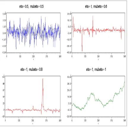
To illustrate the implications of unit-root for an RCA(1) model, we generate four series according to Equation (1.6) with the following set of parameter values,

1. α= 0, σ2 = 1, µβ = 0.5, σβ2 = 0.25

2. α= 0, σ2 = 1, µβ = 0.6, σ_β2 = 0.64

3. α= 0, σ2 = 1, µβ = 0.8, σβ2 = 0.36

4. α= 0, σ2 = 1, µβ = 1, σ2β = 0

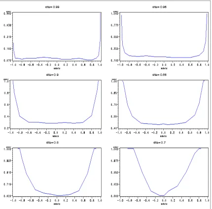
Figure (1.3) shows 500 observations generated for each of the above cases by assum-ing the joint normality of βt and t. Notice only Series 1 is second-order stationary, whereas the other three represent various cases of unit-root non-stationarity. In par-ticular, Series 4 represent a purely random walk process.

Figure 1.2: Comparison of sample path for RCA(1) series with η < 1 and η = 1 (n=500 observations)

series seems to be free to wander, and there is no tendency for the series to be clustered around any fixed level.

RCA(1) and test whether it has a unit root or not.

Chapter 2

Frequentist approach to RCA(1)

models

2.1

Introduction

Consider the RCA(1) model defined in the previous chapter,

xt = α+βtxt−1+t. (2.1)

For this model the following assumptions are made:

A1. {t} is an independent sequence of random variables with mean 0 and variance σ2 >0.

A3. {βt} and {t} are independent.

Before proceeding to derive the properties of RCA(1) model (2.1), let us first give a formal definition of strict stationarity and ergodicity for a stochastic process defined on a probability space (Ω,F, P).

The stochastic process X = (. . . , X₋₁, X₀, X₁, . . .) is said to be strictly stationary

if for any set of random variables {Xt₁, Xt₂, . . . , Xtn} from the collection {Xt : t ∈ T = (0,±1,±2, . . .)} and for any integer h, it is true that,

FX_t1,X_t2,...,X_tn(xt₁, xt₂, . . . , xt_n) = FX_t1+h,X_t2+h,...,X_tn+h(xt₁+h, xt₂+h, . . . , xt_n+h) where FX_t1,X_t2,...,X_tn(xt₁, xt₂, . . . , xt_n) = P(Xt₁ ≤ xt₁, Xt₂ ≤ xt₂, . . . , Xt_n ≤ xt_n) de-notes the joint distribution function of {Xt₁, Xt₂, . . . , Xt_n}.

Given that Y = (. . . , Y₋₁, Y₀, Y₁, . . .) is a strictly stationary random sequence, we need the following concepts to define the ergodicity of Y.

An F − F measurable transformation T: Ω →Ω is said to be measure-preserving

if P(T−1(F)) = P(F) for all F ∈ F. A set F ∈ F is invariant with respect to a transformation T if T−1(F) = F. A measure-preserving transformation T is ergodic

if every invariant set has measure 0 or 1.

2.2

Strict stationarity and ergodicity of RCA(1)

We start by stating a result from Billingsley (1995), which shall be used in the proof for the main theorem of this section.

Lemma 1 Given a stochastic process X = (. . . , X₋₁, X₀, X₁, . . .), define

Y = (. . . , Y₋₁, Y₀, Y₁, . . .) in terms of X by Yn = Φ(. . . , Xn₋₁, Xn, Xn₊₁, . . .). If X is strictly stationary and ergodic, in particular if the Xn’s are independent and

identi-cally distributed, then Y is strictly stationary and ergodic.

Proof. See Theorem 36.4 of Billingsley (1995) for more details. 3

Quinn(1982) considers the problem of the existence of a strictly stationary and ergodic solution to the class of bilinear equations,

Xn =aXn−1+benXn−1+en

where{en}is a sequence of strictly stationary and ergodic random variables. He gives the sufficient and necessary condition to beE(ln|a+ben|)<0 and E(ln|a+ben|)≤0 respectively. Similar arguments can be applied to other types of non-linear discrete time stochastic equations. The following theorem provides one such case which is closely related to the RCA(1) (2.1) we are considering.

Theorem 1 Consider the following class of equations,

Yn = βnYn−1+en, (2.2)

t=n, n-1, . . .}. If E(ln|βn|) < 0, then there exists a strictly stationary and ergodic

solution {Yn} to (2.2), and Yn is measurable with respect to Fn.

Proof. Assume E(ln|βn|) = a < 0. Define the sequence {Tj} by T0 = en, and Tj =j_i=0−1βn₋ien₋j, for j = 1,2, . . ., and let Sr =r_j=1Tj,then we have

ln|Tj| = j−1

i=0

ln|βn₋i|+ln|en₋j|.

By Ergodic theorem, asj → ∞, 1 jln|Tj|

a.s.

−→E(ln|βn|)

and

|Tj|

1

j −→a.s. _exp[E(ln|_βn|_{)] =exp(a)<1}

Now take any realization {T_j} for which the above convergence holds. Then given δ >0, such that δ+a < ρ <1 for some ρ, we can find anRδ such that |Tj|< ρj for j > Rδ. Hence

r j=0|T

j| converges and consequentlySr = r

j=1Tj converges a.s. as r→ ∞.

Now let

Y_n = lim

r→∞Sr =en+

∞

j=1 j−1

i=0

βn−ien−j.

It is obvious thatY

n is aFn-measurable solution to Equation (2.2). Furthermore, by assumption, {en, βn} is stictly stationarity and ergodic, we have {Yn} to be strictly stationary and ergodic according to Lemma (1). 3

are identically distributed sequences, then the weakly stationary solution is also a strictly stationary and ergodic one. We will extend their result to the cases of RCA(1) models whose parameters lie on the region which includes the boundary region of weak stationarity as the interior. This extension turns out to be a crucial result to derive the asymptotic properties of the Maximum Likelihood type of estimators.

In practice, for a RCA(1) model, the sufficient condition in Theorem (1) is not easy to verify for certain distribution ofβt. However, whenβtis normally distributed, the sufficient condition E(ln|βt|)<0 can be evaluated to get an explicit expression.

Theorem 2 Consider the RCA(1) model (2.1) with {βt, t} satisfying assumptions A1−A3. Assume further that {βt, t} are identically normally distributed. Then the sufficient condition for the existence of a strictly stationary and ergodic solution is

that

ln(σ_β2) < ζ +ln(2)−2 ₁

0

1−exp[−λ(1−w2)]

1−w2 dw, (2.3)

where ζ ≈0.57721, denotes the Euler’s constant and λ=µ2_β/2σ2_β.

Proof. Let et = α+t, then {βt, et} is a sequence of stictly stationary and ergodic random vectors. It is trivial to see that E|ln|et|| < ∞ and E|ln|βt|| < ∞. In order to appeal to Theorem (1), we need to show E(ln|βt|) =E(ln|µβ +σβvt|)<0, where vt ∼N(0,1). Now consider the following two situations:

I) If µβ = 0, then

E(ln|βt|) =E(ln|σβvt|) =ln|σβ|+E(ln|vt|) = 1 2ln(σ

2

β)− 1

II) Ifµβ = 0, then

E(ln|βt|) =E(ln|µβ+σβvt|) = 1 2ln(µ

2

β) +E(ln|1 +Z|)

where Z ∼ N(0,σ_µβ2₂

β). An evaluation of E(ln|1 +Z|), see Page 250 of Quinn (1982)

for a similar derivation, gives that,

E(ln|βt|)<0 ⇐⇒ ln(σβ2)< ζ +ln(2)−2 ₁

0

1−exp[−λ(1−w2)] 1−w2 dw.3 Theorem (2) shows that there exists a strictly stationary and ergodic solution of the formxn=en+

_∞ j=1

j₋₁

i=0 βn−ien−j to a RCA(1) model when the parameters lie in the region given by Inequality (2.3). This is demonstrated in Figure (2.1). The shaded area (excluding the upper bound curve) represents the region of strict stationarity and ergodicity. It is easily seen that the region for second-order stationarity (lower left triangle region in light color, see Theorem (3) in Section 2.3) is contained in the region of strict stationarity and ergodicity, and that the boundary region of second-order stationarity µ2_β +σ_β2 = 1 and σ_β2 = 0 lies in the interior of region for strict stationarity and ergodicity.

2.3

Maximum likelihood method

Figure 2.1: Region of strict stationarity and ergodicity for RCA(1)

Theorem 3 Let Ft denote the σ-field generated by {(βs, s), s ≤ t}. There exists a

unique Ft-measurable weakly stationary solution to (2.1) if and only if µ2β+σβ2 <1.

Now, given an RCA(1) process to be weakly stationary, Nicholls and Quinn, hence-forth NQ, show that the Maximum Likelihood estimators are strongly consistent and satistfy a central limit theorem. In this section, we will extend these results to a broader class of model whose parameters can be taken on the space which includes the boundary region of weak stationarity, namely,µ2_β+σ_β2 ≤1 and σ_β2 = 0.

refer to the estimates obtained in this way as the ML estimates, even though it can be shown that all asymptotic results will hold for {βt} and {t} to be non-normal but satisfy the conditions in Theorem (1). In NQ’s work, the assumption of strict stationarity and ergodicity plays a crucial role in deriving the asymptotic results of ML estimators. In Theorem (2) we have shown that the boundary region for second-order stationarity is contained in the region for strict stationarity except for the random walk case, hence most of the results in NQ can be generalized to be applicable for the case of RCA(1) model with a unit root.

Let us denote Θ to be the space over which the parameters of an RCA(1) model is defined. The following assumptions are needed to set further restriction on Θ, which are necessary in proving the consistency and asymptotic normality of the ML estimates.

A4. E(4_t)<∞ and E(β_t4)<∞.

A5. σ2 ≥δ₁ >0 andσ_β2 ≥δ₂ >0, whereδ₁ and δ₂ can be taken as small as required.

A6. (µβ, σβ2) ∈ D, where D can be any closed set contained in the region of strict stationarity and ergodicity given by Inequality (2.3).

Assumption A4 will be used in proving a central limit theorem for ML estimators, and assumptions A5−A6 are imposed so that the space

over which the parameters of RCA model is defined is compact, hence certain results from real analysis can be used in proving the strong consistency of ML estimators. We will derive the asymptotic results of ML estimates of RCA(1) models under as-sumptions A1-A6.

2.3.1

The computation of Maximum Likelihood Estimates

Consider a sample x₀, x₁, . . . , xn from a time series {Xt} which is strictly stationary, ergodic, Ft-measurable and satisfy Equation (2.1) under condition A1-A6. Condi-tional on the known and fixed value x₀, we shall derive the likelihood function by assuming the joint normality ofβt and t. From (2.1), it is easily seen that

E(xt|xt−1) = α+µβxt−1

and

V ar(xt|xt−1) =σ2+σ2βx2t−1, hence the likelihood function (conditional on x₀) has the form:

fn(x1, . . . , xn|x0) = n

i=1

f(xt|xt−1)

= (2π)−n2

n

t=1

(σ2+σ_β2x2_t−1)−12_exp

−(xt−α−µβxt−1)2 2(σ2+σ_β2x2_t−1)

.

= Ln(α, µβ, σβ2, σ2)

Define

˜

ln(α, µβ, σβ2, σ2) = − 2

nln[Ln(α, µβ, σ

2

= 1 n

n

t=1

ln(σ2+σ2_βx2_t−1)− 1 n

n

t=1

(xt−α−µβxt−1)2 σ2+σ2_βx2_t−1

(2.4)

It is more convenient to minimize ˜ln(α, µβ, σ2β, σ2) instead of maximizing Ln(α, µβ, σβ2, σ2). Furthermore, if we re-parameterize τ =

σ2_β

σ2 , we may be able to minimize a function of τ alone, by concentrating out the parameters α, µβ and σ2. Let ¯ln(α, µβ, τ, σ2) = ˜ln(α, µβ, σβ2, σ2), and we have

¯

ln(α, µβ, τ, σ2)

= ln(σ2) +n−1 n

t=1

ln(1 +τ x2_t−1) +σ−2n−1 n

t=1

(xt−α−µβxt−1)2 1 +τ x2_t−1

(2.5)

Now the first derivatives of ¯ln(α, µβ, τ, σ2) with respect to the first three parameters are:

∂ ∂α

¯

ln(α, µβ, τ, σ2) = −2σ−2n−1 n

t=1

xt−α−µβxt−1 1 +τ x2_t−1 , ∂

∂µβ ¯

ln(α, µβ, τ, σ2) = −2σ−2n−1 n

t=1

(xt−α−µβxt−1)xt−1 1 +τ x2_t−1 , and

∂ ∂σ2

¯

ln(α, µβ, τ, σ2) =σ−2−σ−4n−1 n

t₌₁

(xt−α−µβxt−1)2 1 +τ x2_t−1 . Now we have

∂ ∂(α, µβ, σ2)

¯

ln(α, µβ, τ, σ2) = 0 only if

α=αn(τ) =

c₃ −µβ,n(τ)c4 c₁ , and

σ2 =σ_n2(τ) =n−1 n

t=1

[xt−αn(τ)−µβ,n(τ)xt−1]2 1 +τ x2_t−1 , where

c₁ = n

t=1 1

1 +τ x2_t−1, c2 = n

t=1

xtxt−1

1 +τ x2_t−1, c3 = n

t=1

xt 1 +τ x2_t−1, c₄ =

n

t=1

xt−1

1 +τ x2_t−1, c5 = n

t=1

x2_t−1

1 +τ x2_t−1 and c6 = n

t=1

x2_t 1 +τ x2_t−1.

The ML estimates of ˆαn, µˆβ,n, σˆn2 and ˆσ2β,n can be obtained by calculating ˆτn, where ˆ

τn is the minimizer of the following function of τ,

gn(τ) = ln[σn2(τ)] +n−1 n

t=1

ln(1 +τ x2_t−1)

That is, we have profiled the log-likelihood as a function of τ only. This function is nonlinear with respect to τ, and the minimization can be readily done by any numerical routines.

Alternatively, we may consider minimizing the function

ln(α, µβ, τ) = inf σ2

¯_l

n(α, µβ, τ, σ2)−1 = n−1

n

t=1

ln(1 +τ x2_t−1) +ln

n−1 n

t=1

(xt−α−µβxt−1)2 1 +τ x2_t−1

(2.6)

The ML estimates ˆαn, ˆµβ,n, ˆσ2n and ˆσβ,n2 are obtained by

ln( ˆαn,µˆβ,n,τˆn) = inf

ˆ

σ2_n=n−1 n

t=1

(xt−αˆn−µˆβ,nxt−1)2 1 + ˆτnx2t−1 and

ˆ

σ2_β,n= ˆσ_n2τˆn.

2.3.2

The strong consistency of Maximum Likelihood

Esti-mates

The strong consistency of ˆαn, ˆµβ,n, ˆσn2 and ˆσ2β,n will be shown by means of examining the function ln(α, µβ, τ). It should be noted that the minimizer of ln(α, µβ, τ) is the same as the minimizer of l_n(α, µβ, τ) defined by

l_n(α, µβ, τ) = ln(α, µβ, τ)−ln(α0, µβ,0, τ0) = n−1

n

t=1 ln

1 +τ x2_t−1 1 +τ₀x2_t−1

+ln

n−1

n

t=1

(xt−α−µβxt−1)2 1 +τ x2_t−1

−ln

n−1 n

t=1

(xt−α0−µβ,0xt−1)2 1 +τ₀x2_t−1

(2.7)

where α₀, µβ,0 and τ0 denote some fixed values of α, µβ and τ.

Lemma 2 (Ergodic Theorem) Let ξ = (ξ₁, ξ₂, . . .) be a strictly stationary and er-godic random sequence with E|ξ₁|<∞. Then

lim n→∞

1 n

n

k=1

ξk(ω) = E(ξ1) almost surely.

.

Proof. See Theorem 3 of Chapter 5 of Shiryaev (1996). 3 The following result similar to Lemma 3.1 in NQ will be used in proving the main theorem of this section. We will state it without giving the proof. Readers are referred to Nicholls and Quinn (1982) for more details.

Lemma 3 Under Assumption A1-A3, the random variable Yt defined by Yt = Xt2

is non-constant almost surely for all t, where Xt is a strictly stationary and ergodic

solution to Equation (2.1).

The following Lemma is useful in the proofs of the strong consistency and asymp-totic normality of the ML estimators.

Lemma 4 Consider the function of the following form

g(x) = ax

2_+bx+c

dx2+e

where d >0 and e >0. There exists a constant M >0 such that |g(x)| ≤M for any

x.

Proof. Take M =a_d+ b

2√de

Theorem 4 Let {xt}be a strictly stationary, ergodic, Ft-measurable sequence which

satisfies Equation (2.1) with θ = (α, µβ, σβ2, σ2) = (α0, µβ,0, σβ,20, σ02) = θ0 under

conditions A1-A3 and A5-A6. Define π = (α, µβ, τ), where τ = σ2_β

σ2. Let Θ

_{be the}

image ofΘfrom the continuous mappingT :θ→π, whereΘis defined in the previous section. Let π₀ = (α₀, µβ,0, τ0), where τ0 =

σ_β,2₀

σ₀2 . Then limn→∞l

n(α, µβ, τ) exists

almost surely for all (α, µβ, τ) ∈ Θ and the limit l(α, µβ, τ) is uniquely minimized

over Θ _{at π}

0 provided that π0 ∈int(Θ).

Proof. First, Lemma 4.1 in NQ shows that under assumptions A1-A3 and A5-A6 the set Θ is a compact set for suitable δ₁ and δ₂, and δ₁ and δ₂ may be chosen so that (α₀, µβ,0, σβ,20, σ02) ∈int(Θ). SinceT is a continuous mapping and Θ is compact, we also have Θ to be compact and π₀ ∈ int(Θ). Now, by Ergodic Theorem, the three terms in l

n(α, µβ, τ) converge toE

ln

_{1+τ x2}

t−1

1+τ0x2_t−1

,ln

E

(xt−α−µ_βxt−1)2

1+τ x2_t−1 and ln E

(x_t−α₀−µ_β,0x_t−1)2

1+τ₀x2_t−1

respectively, provided the expectations exist. For the first term, it is easy to see that

max

1, τ τ₀

≥ 1 +τ x2t−1

1 +τ₀x2_t−1 ≥min 1, τ τ₀ hence E ln

_{1+τ x2}

t−1

1+τ₀x2_t−1

is finite. For the second term, by Lemma (4) we have

E

(xt−α−µβxt−1)2 1 +τ x2_t−1

=E(xt−α−µβxt−1)

2

1 +τ x2_t−1

≤E(xt−α−µβxt−1)

2

1 +τ x2_t−1 <∞.

For the third term, we have

0< E

(xt−α0−µβ,0xt−1)2 1 +τ₀x2_t−1

Moreover, E[(xt−₁₊α−_{τ x}µβ2xt−1)2

t−1 ] is strictly greater than 0, for otherwise, we would have

xt=α+µβxt−1 = 0 almost surely, which is excluded by Assumption A5 and A6. Now applying the Ergodic Theorem, we have thatl_n(α, µβ, τ) converges almost surely to

l(α, µβ, τ) = E

ln

1 +τ x2_t−1 1 +τ₀x2_t−1

+ln

E

(xt−α−µβxt−1)2 1 +τ x2_t−1

−ln(σ₀2)

Now

E

(xt−α−µβxt−1)2 1 +τ x2_t−1

=E

[(xt−α0−µβ,0xt−1) + (α0−α) + (µβ,0−µβ)xt−1]2 1 +τ x2_t−1

=E

(xt−α0−µβ,0xt−1)2 1 +τ x2_t−1

+E

[(α₀−α) + (µβ,0−µβ)xt−1]2 1 +τ x2_t−1

≥E _σ2

0+σβ,20x2t−1 1 +τ x2_t−1

=σ2₀E

1 +τ₀x2_t−1 1 +τ x2_t−1

,

and the equality will hold in the above only when (α₀ −α) + (µβ,0 −µβ)xt−1 = 0 almost surely, that is whenα=α₀ andµβ =µβ,0 sincext−1 is a non-constant random variable by Lemma(3). Hence,

inf

(α,µ_β)

l(α, µβ, τ) = l(α0, µβ,0, τ)

= E

ln

1 +τ x2_t−1 1 +τ₀x2_t−1

+ln

E

1 +τ₀x2_t−1 1 +τ x2_t−1

and l(α, µβ, τ) = inf(α,µ_β)l(α, µβ, τ) only atα =α0 and µβ =µβ,0.

Now for any non-negative random variable Y with expectation 1, we haveE[ln(Y)]≤ ln[E(Y)] = 0 by Jensen’s Inequality, with equality holding good only when Y = 1 almost surely. Let W =c−1 1+₁₊τ_{τ x}0x22t−1

t−1, wherec=E

1+τ₀x2_t−1

1+τ x2_t−1

.Clearly E(W) = 1 and

inf

(α,µ_β)l

(α, µβ, τ) = E[−ln(cW)] +ln(c) = −E[ln(W)]

with equality holding only when

W =c−11 +τ0x

2

t−1 1 +τ x2_t−1 = 1

almost surely, that is, when (τ₀ −cτ)x2_t−1 + (1 +c) = 0 almost surely. By Lemma (3), this occurs only when τ₀−cτ = 0 and 1−c= 0, that is, when τ = τ₀. Hence, l_{(α, µ}

β, τ) is uniquely minimized at α=α0, µβ =µβ,0 and τ =τ0. 3

Corollary 1 limn_→∞˜ln(α, µβ, σ_β2, σ2) exists almost surely and is minimized uniquely at α=α₀, µβ =µβ,0, σβ2 =σβ,20 and σ2 =σ02.

Proof. First recall that

l_n(α, µβ, τ) = ln(α, µβ, τ)−ln(α0, µβ,0, τ0) = inf

σ2 ¯

ln(α, µβ, τ, σ2)−1−ln(α0, µβ,0, τ0) = inf

σ2 ˜

ln(α, µβ, σβ2, σ2)−1−ln(α0, µβ,0, τ0).

Following Theorem (4) and the definition of ln(α, µβ, τ), it is seen that

limn→∞˜ln(α, µβ, σ2β, σ2) exists almost surely and is uniquely minimized at α = α0, µβ =µβ,0 and σ2 =σ2 =E[(xt−α0−µβ,0xt−1)2/(1 +τ0x2t−1)] and σβ2 =τ0σ2. But

σ2 =E{E[(xt−α0−µβ,0xt−1)2|Ft−1]/(1 +τ0x2t−1)}

=E[(σ₀2+σ_β,2₀x2_t−1)/(1 +τ₀x2_t−1)] = σ2₀.

Theorem(4) is the main result needed in the proof of the following theorem, which states the strong consistency of ML estimates. The proof of this theorem can be given in a similar fashion as that of Theorem 4.2 in NQ. So we will omit the proof. Readers are referred to Nicholls and Quinn (1982) for more details.

Theorem 5 Let ln(α, µβ, τ)be minimized over Θ at α= ˆαn, µβ = ˆµβ,n andτ = ˆτn,

where Θ is defined in Theorem (4). Let πˆn = ( ˆαn,µˆβ,n,τˆn). Then ˆπn converges

almost surely to π₀ = (α₀, µβ,0, τ0)provided that π0 ∈int(Θ). Moreover,σˆβ,n2 and ˆσ2n

converge almost surely to σ2_β and σ2 respectively.

2.3.3

The Central Limit Theorem

First we provide a version of Martingale Central Limit Theorem, see Billingsley (1961), which will be useful in deriving the asymptotic distributions of Maximum Likelihood estimators for an RCA(1) model.

Theorem 6 Let {ξt}be a sequence of random variables with the property that ξt may

be expressed as a function, independent of t, which is measurable with respect to the

σ-field Ft generated by a sequence {αt, αt−1, . . .} of strictly stationary and ergodic

random variables. Furthermore, suppose that E(ξt|Ft−1) = 0 and E(ξt2) = c2 < ∞,

then(c2n)−12 n_t=1ξt converges in distribution to a standard normal random variable.

Proof. Omitted. See Billingsley (1961). 3

˜

ln(α, µβ, σ2β, σ2) to derive a central limit theorem for ˆθn = ( ˆαn,µˆβ,n,σˆβ,n2 ,σˆ2n), the ML estimates ofθ= (α, µβ, σβ2, σ2).Now letθ0 = (α0, µβ,0, σ2β,0, σ02) denote the true values of the parameters. We will prove a central limit theorem forn12(ˆθn−θ0).Before doing that, let us first consider the following lemmata.

Lemma 5 Let fn(θ) be a sequence of continuous and differentiable functions on a

compact set Θ. If limn→∞supθ∈Θ ∂fn(θ)

∂θ

<∞, then fn(θ) is equicontinuous on Θ.

Proof. We need to show that for any > 0, there exists an integer N and a δ >0, both depending on, such that|fn(θ1)−fn(θ2)|< forn > N whenever||θ1−θ2||< δ. Since fn(θ) is continuous and differentiable on Θ, by Mean Value Theorem, we have for θ₁, θ₂ ∈Θ,

fn(θ1)−fn(θ2) = (θ1 −θ2)

∂fn(θ) ∂θ where θ _=λθ

1+ (1−λ)θ2 for some λ∈(0,1). Now since

(θ₁−θ₂)∂fn(θ ₎ ∂θ

2 ≤ ||θ₁−θ₂||2∂fn(θ ₎ ∂θ

2,

it will follow thatfn(θ) is equicontinuous if limn→∞supθ∈Θ ∂fn(θ)

∂θ

<∞. 3

The above stated lemma can be used to show the equicontinuity of the second derivative of ˜ln(θ), {∂

2˜l_n(θ)

∂θ∂θ }, on a compact neighborhood N(θ0) of θ0. Following the lemma, it suffices to show each element of the third derivative of ˜ln(θ) is uniformly bounded on N(θ₀). For example, for

∂2˜ln(θ) ∂µ2_β = 2n

−1

n

t=1

where λt=σ2+σβ2x2t−1, we have

∂3˜ln(θ) ∂µ2_β∂σ2

= 2n−1| n

t₌₁

λ−_t2x2_t−1|

≤ 2n−1 n

t=1

|λ−_t1x2_t−1||λ−_t1|

≤ 2

σ_β2σ2. < ∞

Similar argument can be made term by term for other elements of the derivative of

{∂2˜ln(θ) ∂θ∂θ }.

Lemma 6 Let {θn} be a sequence of random variables such that θn converges to θ0

almost surely for some constant value θ₀. Let {fn(.)} be a sequence of functions

such that fn(θ)converges to a continuous function f(θ) uniformly almost surely on a

neighborhood N(θ₀) of θ₀. Then we have that fn(θn)converges to f(θ0) almost surely. Proof. Take any ω for which θn(ω) converges to θ0(ω), then for n sufficiently large, we have θn(ω)∈N(θ0). Now fix ω, we have

|fn(θn)−f(θ0)| = |fn(θn)−f(θn) +f(θn)−f(θ0)|

≤ |fn(θn)−f(θn)|+|f(θn)−f(θ0)|

The first term in the above inequality can be bounded by an arbitrary small number, say /2, because of the uniform convergence of fn(.) to f(.) on the neighborhood

N(θ₀) ofθ₀. The second term can be bounded by/2 because of the continuity off(.) onN(θ₀). Hence by taking n sufficiently large, we have

hence fn(θn) converges to f(θ0) almost surely. 3

Lemma 7 The sequence {∂_∂θ∂θ2˜ln(θ)} converges uniformly almost surely on a compact neighborhood N(θ₀) of θ₀ to {∂_∂θ∂θ2˜l(θ)}, where ˜l(θ) = limn→∞˜ln(θ).

Proof. First, define λt=σ2+σβ2x2t−1 and ut =xt−α−µβxt−1. We have

E(ut|Ft₋₁) = E[(xt−α₀−µβ,₀xt₋₁) + (α₀−α) + (µβ,₀−µβ)xt₋₁|Ft₋₁] = α₀−α+ (µβ,0−µβ)xt−1

and

E(u2_t|Ft−1) = E{[(xt−α0−µβ,0xt−1) + (α0−α) + (µβ,0−µβ)xt−1]2|Ft−1} = σ₀2+σ2_β,0x2_t−1+ [(α₀−α) + (µβ,0−µβ)xt−1]2.

Now the second derivative of ˜ln(θ) is element-wise given by, ∂2˜ln(θ)

∂α2 = 2n

−1

n

t=1 λ−_t1, ∂2˜ln(θ)

∂α∂µβ

= 2n−1 n

t=1

λ−_t1xt−1, ∂2˜ln(θ)

∂α∂σ_β2 = 2n

−1

n

t=1

λ−_t2utx2t₋₁, ∂2˜ln(θ)

∂α∂σ2 = 2n

−1

n

t=1

λ−_t2ut, ∂2˜ln(θ)

∂µ2_β = 2n

−1

n

t=1

λ−_t1x2_t−1, ∂2˜ln(θ)

∂µβ∂σ2_β

= 2n−1 n

t=1

λ−_t2utx3t−1, ∂2˜ln(θ)

∂µβ∂σ2

= 2n−1 n

t=1