Pak.j.stat.oper.res. Vol.XIII No.3 2017 pp501-528
under Different Loss Functions
Tabasam Sultana
Department of Statistics, Quaid-i-Azam University, Islamabad, Pakistan [email protected]
Muhammad Aslam
A Department of Basic Sciences, Ripha International University, Islamabad, 44000, Pakistan [email protected].
Javid Shabbir
Department of Statistics, Quaid-i-Azam University, Islamabad, Pakistan [email protected]
Abstract
This paper has to do with 3-component mixture of the Frechet distributions when the shape parameter is known under Bayesian view point. The type-I right censored sampling scheme is considered due to its extensive use in reliability theory and survival analysis. Taking different non-informative and informative priors, Bayes estimates of the parameter of the mixture model along with their posterior risks are derived under squared error loss function, precautionary loss function and DeGroot loss function. In case, no or little prior information is available, elicitation of hyper parameters is given. In order to study numerically, the execution of the Bayes estimators under different loss functions, their statistical properties have been simulated for different sample sizes and test termination times. A real life data example is also given to illustrate the study.
Keywords: Bayes Estimators, Censoring, Informative prior, Loss Functions, Posterior Risks.
1. Introduction
Frechet distribution was introduced by a French mathematician named Maurice Frechet (1878, 1973) who had determined before one possible limit distribution for the largest order statistic in 1927. The Frechet distribution has been manifested to be helpful for modeling and analysis of several extreme events ranging from accelerated life testing to earthquakes, floods, rain fall, sea currents and wind speed.
Several types of data are encountered in everyday life, regarding simple data, grouped data, truncated data, censored data and progressively censored data. Censoring is an inevitable part of the lifetime data. A valuable account of censoring is given in Gijbles (2010) and Kalbfleisch and Prentice (2011). There are different sorts of censoring schemes, including right, left and interval censoring, single or multiple censoring and type-1 and type-II censoring. Kundu and Howlader (2010) discussed the Bayesian inference and prediction of the IW distribution for type-II censored data. Shi and Yan (2010) derived the empirical Bayes estimates of the two parameter exponential distribution under type-I censoring. Saleem et al. (2010) discussed Bayesian analysis on the power function mixture distribution using typeI censored data. Ali (2015) described the 2-component mixture of the inverse Rayleigh distributions under Bayesian framework. Aslam et al. (2015) presented 3-component mixture of Rayleigh distributions, properties and estimation under the Bayesian framework.
Inspired by above mentioned applications of mixture models, we intend to study Bayesian analysis of a 3-component mixture of the Frechet distributions with unknown mixing proportions. The parameters of component distributions are assumed to be unknown. Four different priors and three different loss functions are used for the Bayesian analysis. Moreover, we consider an ordinary type-I right censored sampling schemes.
The structure of this article is as follows. The Frechet mixture model along with its likelihood function is formulated in section 2. The expressions for posterior distributions using the non-informative and informative priors are derived in section 3. In section 4, the Bayes estimators and posterior risks using the uniform, the Jeffreys’, the exponential and the inverse levy priors under squared error loss function (SELF), precautionary loss function (PLF) and DeGroot loss function (DLF) are presented. The elicitation of hyperparameters is given in section 5. In section 6, the limiting expressions of the Bayes estimators and their posterior risks are derived. The simulation study and the real data applications are presented in section 7 and 8, respectively. This article concludes with a brief discussion in section 9.
2. 3-Component mixture of the Frechet distributions
Pak.j.stat.oper.res. Vol.XIII No.3 2017 pp501-528 503 When the shape parameterα = 1, then the above p.d.f and c.d.f will become as:
(3)
(4)
A finite 3-component mixture model with the unknown mixing proportions p1and p2 is:
(5)
(6)
While the c.d.f of 3-component mixture model is:
(7)
(8)
2.1. The Likelihood Function. Suppose ‘n’ units from the 3-component mixture of Frechet distributions are used in a life testing experiment with fixed test termination time t. Let ‘r’ units out of ‘n’ units failed until fixed test termination time ‘t’ and the remaining (n-r) units are still working. According to Mendenhall and Hader (1958), there are many practical situations in which the failed objects can be pointed out easily as subset of subpopulation-I, subpopulation-II or subpopulation-III. Out of ‘r’ units, supposer1, r2 and r3units belong to subpopulation-I, subpopulation-II or subpopulation-III respectively and such that r = r1+r2+r3. Now we definexlk,0 < xlk < t be the failure time of kth unit
belonging to the lth subpopulation, where l = 1,2,3andk = 1, 2, ..., rl. For a 3-component
mixture model, the likelihood function can be written as:
3
1 2
1 1 1 2 2 2 1 2 3 3
1 1 1
( 1 1 (9)
r
r r
n r
k k k
k k k
L x p f x p f x p p f x F t
After simplification, the likelihood function of 3-component mixture of Frechet distributions is given:
(10)
Where X = (x1, x12, ..., x1r1, x21, x22, ..., x2r2, x31, x32, …, x3r3) are the observed failure times
3.1. The posterior distribution using the Uniform Prior (UP). When elicitation of hyper parameters is difficult or little prior information is given, then usually the non-informative prior is assumed to be the UP. Ups over the intervals (0, ∞) and (0,1) are taken for the parameters (β1, β2 &β3) of Frechet distribution and for the mixing proportions (p1, p2) respectively. With these settings, joint prior distribution of parameters (β1, β2, β3, p1, p2), is given by:
π1 (φ) ∝ 1; β1, β2, β3 > 0, p1, p2 ≥ 0, p1 + p2 ≤ 1
The joint posterior distribution of parameters β1, β2, β3, p1 and p2 given data x assuming the UP is:
(11) where
31 31 31 21 21 21 11 11 11 01 01 01 01 010 0 0
1 3 01 2 01 1 01 3 1 1 3 31 2 1 1 2 21 1 1 1 1 11 3 31 2 21 1 11 , , 1 , 1 , 1 , 1 , , , , 1 , 1 , 1 A A A r n i i j j l i r k k r k k r k k M A M A M A C A B B C A B l j j i i r n C r l C r l j B r j i A t l x M t l j x M t j i x M r A r A r A
3.2. The posterior distribution using the Jeffreys’ prior (JP).
According to Jeffreys’ (1946, 1998) and Berger (1985), the JP is defined as
I ,m1,2,3
pm m , where
2 2 m m m x f E I
Pak.j.stat.oper.res. Vol.XIII No.3 2017 pp501-528 505 The joint posterior distribution of parameters β1, β2, β3, p1 and p2 given data x assuming the JP is:
(12) where 32 32 32 22 22 22 12 12 12 02 02 02 02 02 0 0 0
2 3 02 2 02 1 02 3 1 1 3 32 2 1 1 2 22 1 1 1 1 12 3 32 2 22 1 12 , , 1 , 1 , 1 , 1 , , , , , , A A A r n i i j j l i r k k r k k r k k M A M A M A C A B B C A B l j j i i r n C r l C r l j B r j i A t l x M t l j x M t j i x M r A r A r A
3.3. The posterior distribution using the Exponential prior (EP). As an informative prior, we take the exponential prior for the component parameters β1, β2, β3 and Bivariate Beta prior for proportion parameters p1, p2. Symbolically, it can be written as: β1 ∼ Exponential(k1), β2 ∼ Exponential(k2), β3 ∼ Exponential(k3) and p1, p2 ∼Bivariate Beta (a, b, c). Again assuming independence of all parameters, the joint prior distribution of (β1, β2, β3, p1, p2) is given by:
The joint posterior distribution of parameters β1, β2, β3, p1 and p2 given data x is:
(13) where 33 33 33 23 23 23 13 13 13 03 03 03 03 03 0 0 0
Beta (a, b, c). Again assuming independence of all parameters, the joint prior distribution of (β1, β2, β3, p1, p2) is given by:
The joint posterior distribution of parameters β1, β2, β3, p1 and p2 given data x is:
(14) where 34 34 34 24 24 24 14 14 14 04 04 04 04 04 0 0 0
4 3 04 2 04 1 04 3 3 1 1 3 34 2 2 1 1 2 24 1 1 1 1 1 14 3 34 2 24 1 14 , , 1 , , , , 2 , 2 , 2 , 2 1 , 2 1 , 2 1 A A A r n i i j j l i r k k r k k r k k M A M A M A C A B B C A B l j j i i r n C c r l C b r l j B a r j i A a t l x M a t l j x M a t j i x M r A r A r A
4. Bayes estimators and posterior risks using the UP, the JP, the Exponential and Inverse Levy prior under SELF, PLF and DLF
If dˆ is a Bayes estimator, then
dˆ is called posterior risk and is defined as:
dˆ E |x
L
,dˆ
. Our purpose, in this study, is to look for efficient Bayes estimates of the different parameters. For this purpose, three different loss functions, namely SELF, PLF and DLF used to obtain Bayes estimators and their posterior risks. The SELF, defined as
,d d2
L ,was introduced by Legendre to develop the least squares theory. Norstrom
(1996) discussed an asymmetric PLF and also introduced a special case of general class
of PLFs, which is defined as
d d d L 2 ,
Pak.j.stat.oper.res. Vol.XIII No.3 2017 pp501-528 507
where v=1 for the UP, v=2 for the JP, v=3 for the EP and v=4 for the ILP.
4.2. The Bayes estimators and posterior risks using the UP, the JP and IP under PLF. Norstrom (1996) discussed an asymmetric PLF and also introduced a special case
of general class of PLFs, which is defined as
d d d
L
2
,
. The Bayes estimator and
posterior risk are:
Ex
d
Ex
Ex d 2 |
1 2 | 2
1 2
| , ˆ 2 2
ˆ , respectively. The respective marginal posterior
Pak.j.stat.oper.res. Vol.XIII No.3 2017 pp501-528 513
5. Elicitation of Hyper-parameters
Elicitation is the main task for subjective Bayesian. The complete procedure for quantifying the prior information in the form of prior distribution is precisely known as the elicitation. Aslam (2003) presented different methods of elicitation based on prior predictive distribution for the elicitation of the hyper-parameters. In this study, we use the method of elicitation using prior predictive distribution based on the predictive probabilities. In this approach, confidence levels of the prior predictive are gained for the particular intervals of the random variables. The set of hyper parameters, for which the difference between the elicited probabilities and the expert predictive probabilities is minimum, is considered.
5.1. Elicitation of hyper-parameters using the Exponential Prior. For eliciting the hyper-parameters, prior predictive distribution (PPD) is used. The PPD for a random variable X is:
(15)
(16)
For eliciting the hyper parameters k1, k2, k3, a, b and c and the equations are simultaneously solved through the computer program developed in SAS package using the ‘PROC SYSLIN’ command, the values of the hyper parameters are found to be 2.0003,3.0030,4.0016,2.0103,1.7607and 1.50 respectively.
5.2. Elicitation of hyper parameters using the Inverse Levy Prior. The PPD using Inverse Levy prior for a random variable X is given by:
(17)
(18)
Using same canon defined as above for the exponential prior, the values of the hyper-parameters a1, a2, a3, a, b and c are 1.9520, 2.5321, 3.7735, 0.2763, 0.1167 and 1.0.
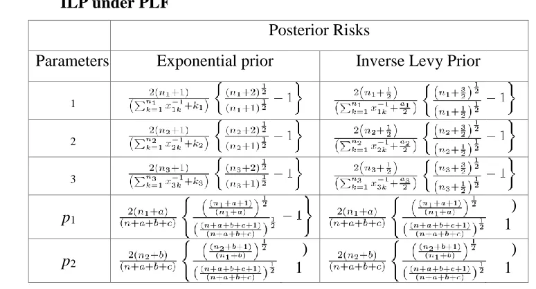
6. Limiting Expressions. Letting t → ∞, all the observations that are assimilated in our analysis are uncensored and therefore r tends n, r1tends to the unknown n1, r2tends to the unknown n2 and r3tends to the unknown n3. As a result, the amount of information carried in the sample expands, which results in the depletion of the variances of the estimates. The limiting (complete sample) expressions for Bayes estimators and posterior risks using the UP, the JP, the EP and the ILP under SELF, PLF and DLF are given in the Tables 1-6.
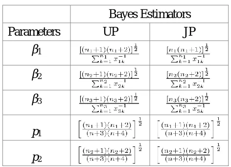
Table 1: Limiting Expressions for the Bayes Estimators as t →∞ assuming the UP, the JP and the IP under SELF
Bayes Estimators
Parameters UP JP Exponential prior Inverse Levy Prior
Pak.j.stat.oper.res. Vol.XIII No.3 2017 pp501-528 515
Table 2: Limiting Expressions for the Bayes Estimators as t →∞ using the UP and the JP under PLF
Bayes Estimators
Parameters UP JP
β1
β2
β3
p1
p2
Table 3: Limiting Expressions for the Bayes Estimators as t →∞ using the EP and the ILP under PLF
Bayes Estimators
Parameters Exponential Prior Inverse Levy Prior β1
β2
β3
p1
p2
Table 4: Limiting Expressions for the Bayes Estimators as t →∞ using the UP and the JP, EP and ILP under DLF
Bayes Estimators
Parameters UP JP Exponential Prior Inverse Levy Prior
β1
β2 β3
p1
4 2
1
n n
4 2
1
n n
p2
4 2
2
n n
4 2
2
n n
c b a n
b n
1
2
c b a n
b n
1
β1
β2
β3
p1
p2
Table 6: Limiting Expressions for the Posterior risks as t →∞ using the UP and the JP under PLF
Posterior Risks
Parameters UP JP
β1
β2
β3
p1
p2
Table 7: Limiting Expressions for the Posterior risks as t →∞ using the EP and ILP under PLF
Posterior Risks
Parameters Exponential prior Inverse Levy Prior
Pak.j.stat.oper.res. Vol.XIII No.3 2017 pp501-528 517
7. Simulation Study
A comprehensive simulation study was conducted in order to explore the performance of the Bayes estimators, impact of sample size and censoring rate to be appropriate for the model. Samples of sizes n=25, 40, 55 are generated from a 3-component mixture of the Frechet distributions with various set of the parametric values β1, β2, β3, p1 and p2 fixed as (β1, β2, β3, p1, p2) = (0.50, 1.0, 1.50, 0.30, 0.50), (1.50, 1.0, 0.50, 0.50, 0.30). For fixed sample size, test termination time and set of parameters, the simulation is repeated 1000 times and the results are then averaged. Sample of sizes p1n, p2n and (1 − p1 − p2) n are chosen randomly from first component densityf1 (x; θ1), second component density f2 (x; θ2) and third component densityf3 (x; θ3), respectively.
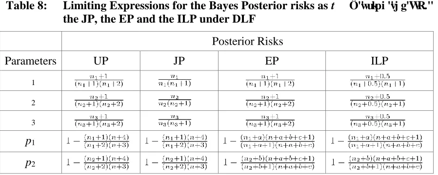
Table 8: Limiting Expressions for the Bayes Posterior risks as t →∞ using the UP, the JP, the EP and the ILP under DLF
Posterior Risks
Parameters UP JP EP ILP
β1 β2 β3
p1
p2
The observations which are greater than a fixed t are declared as censored observations. For each t only failures have been inspected either as a member of subpopulation-I or subpopulation-II or subpopulation-III. On the basis of each sample size, the Bayes estimators (BEs) and Posterior risks (PRs) are computed using the informative and non-informative priors under SELF, PLF and DLF. In order to conduct Bayesian analysis under informative priors, elicitation of hyper-parameters is obtained by using the prior predictive approach. In order to evaluate the impact of test termination time on Bayes estimators, the Type-I right censoring scheme is used for fixed test termination time t=15 and 20. For each of the 1000 samples, the Bayes estimators and Posterior risks were calculated using a routine in Mathematica 10.0 and the results are presented in Tables 9-16. The simulation study gives us some interesting characteristics of the Bayes estimates. The properties have been foregrounded in terms of sample sizes, size of mixing proportion parameters, different loss functions and censoring rates. It is noticed that because of censoring, the posterior risks of all the parameters are reduced with an increase in sample size.
8. A Real Life Data Application
. 5522 . 13
3 1
1 3
k k x
Bayes estimates and Bayes Posterior risks using the UP, the JP, the EP and the ILP under SELF, PLF and DLF are in Table 17 given in appendix.
It is noted that the results gained from real data are compatible with simulation results. The results declare that the execution of the informative prior is better than the non-informative priors. It is also examined that execution of DLF preferred for estimating the component parameters, while SELF better for estimating the proportion parameters.
9. Final Remarks
In this study, the Bayesian estimation of 3-component mixture of the Frechet distributions has been considered assuming the case when the shape parameter is known based on type-I censored data. The purpose of this paper is to find out the appropriate combinations of prior distributions and loss functions to estimate the parameters of the 3-component mixture of the Frechet distributions. We conducted all-encompassing simulation study to find out the relative performance of the Bayes estimators when the shape parameter is assumed to be known. From simulated results, we observed that an increase in the sample size and test termination time provides better Bayes estimators. Furthermore, as sample size increases (decreases) the posterior risks of Bayes estimators’ decreases (increases) for a fixed test termination time. Also, the DLF is perceived as an appropriate choice for estimating component parameters and SELF is expedient for estimating the proportion parameters. Finally, we deduce that the EP is apt prior in order to estimate the component parameters. When SELF is used, the EP is an appropriate prior for proportion parameters. The similar pattern is examined for the JP when non-informative priors are contemplated.
References
1. Abbas, K. and Y. Tang. Analysis of Frechet Distribution Using Reference Priors, Communications in Statistics-Theory and Methods 44(14), 2945-2956, 2015.
Pak.j.stat.oper.res. Vol.XIII No.3 2017 pp501-528 519 5. Aslam, M. An application of prior predictive distribution to elicit the prior
density, Journal of Statistical Theory and applications 2(1), 70-83, 2003.
6. Aslam, M., Tahir, M., Hussain, Z., & Al-Zahrani, B. A 3-Component Mixture of Rayleigh Distributions: Properties and Estimation in Bayesian Framework, PloS one 10(5), e0126183, 2015.
7. Chatterjee, A., and Chatterjee, A. Use of the Frechet distribution for UPV measurements in concrete, NDT and E International 52, 122-128, 2012
8. Crowder, M. J., A. Kimber, et al. Statistical analysis of reliability data (CRC Press, 1994).
9. DeGroot, M. H. Optimal statistical decisions (John Wiley and Sons, 2005). 10. Frechet, M. Sur la loi de probabilite de lecart maximum, Annales Soc.Polon.
Math 6(95), 1927.
11. Gijbels, I. (2010). Censored data, Wiley Interdisciplinary Reviews: Computational Statistics 2(2), 178-188, 2010.
12. Harlow, D. G. Applications of the Frechet distribution function, International Journal of Materials and Product Technology 17(5-6), 482-495, 2002.
13. Jeffreys, H. An invariant form for the prior probability in estimation problems, Proceedings of the Royal Society of London A: Mathematical, Physical and Engineering Sciences, The Royal Society, 1946.
14. Jeffreys, H. The theory of probability (OUP Oxford, 1998).
15. Kalbfleisch, J. D. and R. L. Prentice. The statistical analysis of failure time data (John Wiley & Sons, 2011).
16. Kundu, D. and H. Howlader. Bayesian inference and prediction of the inverse Weibull distribution for Type-II censored data, Computational Statistics and Data Analysis 54, 1547-1558, 2010.
17. Legendre, A. M. Nouvelles methodes pour la determination des orbites des cometes F. Didot, 1805.
18. Mendenhall, W. and R. Hader. Estimation of parameters of mixed exponentially distributed failure time distributions from censored life test data, Biometrika 45(3-4), 504-520, 1958.
19. Nadarajah, S. and S. Kotz. Sociological models based on Frechet random variables, Quality and Quantity 42 (1), 89-95, 2008.
20. Norstrom, J. G. The use of precautionary loss functions in risk analysis, IEEE Transactions on reliability 45 (3), 400-403, 1996.
21. Saleem, M., Aslam, M., & Economou, P. On the Bayesian analysis of the mixture of power function distribution using the complete and the censored sample, Journal of Applied Statistics 37(1), 25-40, 2010.
22. Shi, Y. and Yan, W. The EB Estimation of Scale-parameter for Two Parameter Exponential Distribution Under the Type-I Censoring Life Test, 2010.
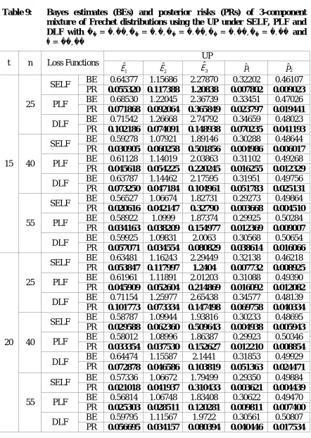
DLF with 𝜷𝟏= 𝟎. 𝟓𝟎, 𝜷𝟐 = 𝟏. 𝟎, 𝜷𝟑 = 𝟏. 𝟓𝟎, 𝒑𝟏= 𝟎. 𝟑𝟎, 𝒑𝟐= 𝟎. 𝟓𝟎 and
𝒕 = 𝟏𝟓, 𝟐𝟎
t n Loss Functions UP
1
ˆ
ˆ2
3
ˆ
pˆ1 pˆ2
15 25
SELF BE 0.64377 1.15686 2.27870 0.32202 0.46107
PR 0.055320 0.117388 1.20838 0.007802 0.009023
PLF BE 0.68530 1.22045 2.36739 0.33451 0.47026
PR 0.071868 0.092064 0.365849 0.023797 0.019441
DLF BE 0.71542 1.26668 2.74792 0.34659 0.48023
PR 0.102186 0.074091 0.148938 0.070235 0.041193
40
SELF BE 0.59278 1.07921 1.89146 0.30288 0.48644
PR 0.030905 0.060258 0.501856 0.004986 0.006017
PLF BE 0.61128 1.14019 2.03863 0.31102 0.49268
PR 0.045618 0.054225 0.220245 0.016255 0.012329
DLF BE 0.63787 1.14462 2.17595 0.31951 0.49756
PR 0.073250 0.047184 0.104961 0.051783 0.025131
55
SELF BE 0.56527 1.06674 1.82731 0.29273 0.49864
PR 0.020616 0.042147 0.32790 0.003668 0.004510
PLF BE 0.58922 1.0999 1.87374 0.29925 0.50284
PR 0.034163 0.038209 0.154977 0.012369 0.009007
DLF BE 0.59925 1.09831 2.0063 0.30568 0.50654
PR 0.057071 0.034554 0.080829 0.038614 0.016066
20 25
SELF BE 0.63481 1.16243 2.29449 0.32138 0.46218
PR 0.053847 0.117997 1.2404 0.007732 0.008925
PLF BE 0.61961 1.11891 2.01203 0.31088 0.49390
PR 0.045909 0.052604 0.214869 0.016092 0.012082
DLF BE 0.71154 1.25977 2.65438 0.34577 0.48139
PR 0.101773 0.073334 0.147498 0.069758 0.040334
40
SELF BE 0.58787 1.09944 1.93816 0.30233 0.48695
PR 0.029588 0.062360 0.509643 0.004938 0.005943
PLF BE 0.58012 1.08996 1.86387 0.29923 0.50346
PR 0.033354 0.037530 0.152627 0.012210 0.008854
DLF BE 0.64474 1.15587 2.1441 0.31853 0.49929
Pak.j.stat.oper.res. Vol.XIII No.3 2017 pp501-528 521
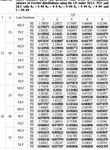
Table 10: Bayes estimates (BEs) and posterior risks (PRs) of 3-component mixture of Frechet distributions using the UP under SELF, PLF and DLF with 𝜷𝟏= 𝟏. 𝟓𝟎, 𝜷𝟐 = 𝟏. 𝟎, 𝜷𝟑 = 𝟎. 𝟓𝟎, 𝒑𝟏= 𝟎. 𝟓𝟎, 𝒑𝟐= 𝟎. 𝟑𝟎 and 𝒕 = 𝟏𝟓, 𝟐𝟎
t n Loss Functions UP
1
ˆ
ˆ2 ˆ3 pˆ1 pˆ2
15 25
SELF BE 1.74859 1.29527 0.75497 0.46006 0.32346
PR 0.270075 0.225689 0.130652 0.009132 0.008040
PLF BE 1.83555 1.35025 0.82037 0.47208 0.33400
PR 0.138592 0.14421 0.12496 0.01961 0.024479
DLF BE 1.90234 1.44896 0.91036 0.48072 0.34776
PR 0.074547 0.104087 0.146394 0.041797 0.072502
40
SELF BE 1.65716 1.19814 0.65269 0.48610 0.30248
PR 0.143936 0.129094 0.056772 0.006090 0.005145
PLF BE 1.70319 1.22146 0.67259 0.49308 0.31114
PR 0.081165 0.092916 0.070894 0.012431 0.016763
DLF BE 1.72312 1.30093 0.73093 0.49883 0.32006
PR 0.047247 0.074745 0.102658 0.025266 0.053523
55
SELF BE 1.60162 1.14253 0.59521 0.49681 0.29308
PR 0.089013 0.086113 0.032680 0.003948 0.003298
PLF BE 1.64833 1.17848 0.63863 0.50219 0.30031
PR 0.057169 0.069427 0.051312 0.009029 0.012717
DLF BE 1.65163 1.21835 0.65325 0.50761 0.30658
PR 0.034042 0.058143 0.079678 0.017355 0.041676
20 25
SELF BE 1.74164 1.26138 0.75824 0.46195 0.32211
PR 0.263732 0.2034 0.132482 0.008973 0.007877
PLF BE 1.82546 1.34552 0.82642 0.47233 0.33397
PR 0.136515 0.141848 0.12488 0.019230 0.024031
DLF BE 1.86253 1.45122 0.85807 0.48077 0.34732
PR 0.073767 0.102882 0.145164 0.040847 0.071070
40
SELF BE 1.66985 1.18325 0.65066 0.48769 0.30177
PR 0.143726 0.123538 0.056842 0.005962 0.005027
PLF BE 1.68955 1.23244 0.69396 0.49364 0.31069
PR 0.079878 0.092856 0.072807 0.012222 0.016509
DLF BE 1.72569 1.26653 0.71998 0.49894 0.31941
PR 0.046851 0.073979 0.101862 0.024806 0.052370
55
SELF BE 1.60023 1.14286 0.60400 0.49943 0.29279
PR 0.094254 0.085622 0.034621 0.004502 0.003697
PLF BE 1.62303 1.1672 0.61780 0.50322 0.29982
PR 0.056158 0.067970 0.049419 0.008894 0.012476
DLF BE 1.65811 1.20219 0.65917 0.50655 0.30703
t n Loss Functions JP
1
ˆ
ˆ2 ˆ3 pˆ1 pˆ2
15 25
SELF BE 0.58091 1.07457 1.85935 0.32217 0.46147
PR 0.051092 0.109223 0.951593 0.007807 0.009032
PLF BE 0.60021 1.13312 2.08241 0.33307 0.47157
PR 0.070939 0.092292 0.381584 0.023884 0.019457
DLF BE 0.65665 1.18461 2.34335 0.34626 0.48170
PR 0.114117 0.079845 0.176529 0.070452 0.041015
40
SELF BE 0.55630 1.05499 1.67388 0.30230 0.48745
PR 0.029581 0.060950 0.43985 0.004982 0.006022
PLF BE 0.56735 1.077 1.83786 0.31062 0.49246
PR 0.045768 0.053800 0.221624 0.016264 0.012335
DLF BE 0.59180 1.11057 1.95818 0.319287 0.49886
PR 0.079044 0.049363 0.117900 0.051770 0.024977
55
SELF BE 0.53448 1.02133 1.66279 0.29362 0.49907
PR 0.019683 0.039942 0.298843 0.003652 0.004498
PLF BE 0.55075 1.04966 1.74973 0.29920 0.50327
PR 0.033769 0.037669 0.158084 0.012287 0.008977
DLF BE 0.57305 1.07198 1.8412 0.30605 0.50608
PR 0.061325 0.036334 0.087157 0.041727 0.01864
20 25
SELF BE 0.57603 1.07749 1.87336 0.32097 0.46305
PR 0.049727 0.109074 0.943486 0.007725 0.008929
PLF BE 0.57162 1.08094 1.80660 0.31099 0.49397
PR 0.045693 0.053343 0.217134 0.016094 0.012096
DLF BE 0.63484 1.16903 2.27552 0.34558 0.48200
PR 0.113312 0.079047 0.173688 0.069736 0.040230
40
SELF BE 0.54322 1.0624 1.73359 0.30293 0.48638
PR 0.027587 0.061416 0.464869 0.004935 0.005931
PLF BE 0.55228 1.05684 1.72704 0.29962 0.50377
PR 0.033652 0.037662 0.154077 0.012207 0.008851
DLF BE 0.58417 1.10718 1.91391 0.31895 0.49892
PR 0.078584 0.048943 0.116287 0.051297 0.024487
SELF BE 0.54156 1.02793 1.64473 0.29325 0.49877
Pak.j.stat.oper.res. Vol.XIII No.3 2017 pp501-528 523
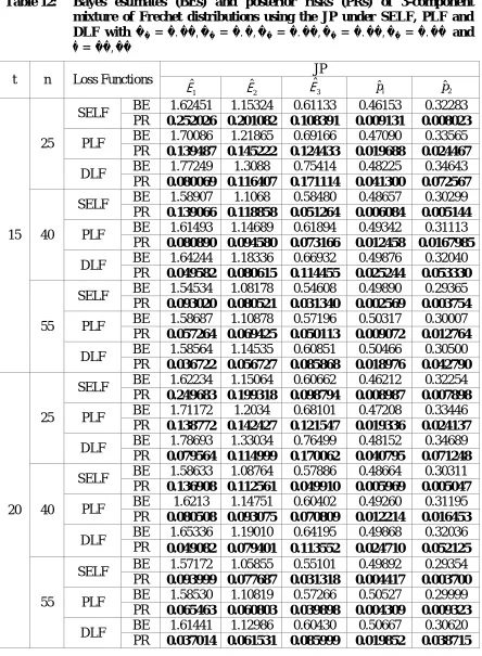
Table 12: Bayes estimates (BEs) and posterior risks (PRs) of 3-component mixture of Frechet distributions using the JP under SELF, PLF and DLF with 𝜷𝟏= 𝟏. 𝟓𝟎, 𝜷𝟐 = 𝟏. 𝟎, 𝜷𝟑 = 𝟎. 𝟓𝟎, 𝒑𝟏= 𝟎. 𝟓𝟎, 𝒑𝟐= 𝟎. 𝟑𝟎 and 𝒕 = 𝟏𝟓, 𝟐𝟎
t n Loss Functions JP
1
ˆ
ˆ2 ˆ3 pˆ1 pˆ2
15 25
SELF BE 1.62451 1.15324 0.61133 0.46153 0.32283
PR 0.252026 0.201082 0.108391 0.009131 0.008023
PLF BE 1.70086 1.21865 0.69166 0.47090 0.33565
PR 0.139487 0.145222 0.124433 0.019688 0.024467
DLF BE 1.77249 1.3088 0.75414 0.48225 0.34643
PR 0.080069 0.116407 0.171114 0.041300 0.072567
40
SELF BE 1.58907 1.1068 0.58480 0.48657 0.30299
PR 0.139066 0.118858 0.051264 0.006084 0.005144
PLF BE 1.61493 1.14689 0.61894 0.49342 0.31113
PR 0.080890 0.094580 0.073166 0.012458 0.0167985
DLF BE 1.64244 1.18336 0.66932 0.49876 0.32040
PR 0.049582 0.080615 0.114455 0.025244 0.053330
55
SELF BE 1.54534 1.08178 0.54608 0.49890 0.29365
PR 0.093020 0.080521 0.031340 0.002569 0.003754
PLF BE 1.58687 1.10878 0.57196 0.50317 0.30007
PR 0.057264 0.069425 0.050113 0.009072 0.012764
DLF BE 1.58564 1.14535 0.60851 0.50466 0.30500
PR 0.036722 0.056727 0.085868 0.018976 0.042790
20 25
SELF BE 1.62234 1.15064 0.60662 0.46212 0.32254
PR 0.249683 0.199318 0.098794 0.008987 0.007898
PLF BE 1.71172 1.2034 0.68101 0.47208 0.33446
PR 0.138772 0.142427 0.121547 0.019336 0.024137
DLF BE 1.78693 1.33034 0.76499 0.48152 0.34689
PR 0.079564 0.114999 0.170062 0.040795 0.071248
40
SELF BE 1.58633 1.08764 0.57886 0.48664 0.30311
PR 0.136908 0.112561 0.049910 0.005969 0.005047
PLF BE 1.6213 1.14751 0.60402 0.49260 0.31195
PR 0.080508 0.093075 0.070809 0.012214 0.016453
DLF BE 1.65336 1.19010 0.64195 0.49868 0.32036
PR 0.049082 0.079401 0.113552 0.024710 0.052125
55
SELF BE 1.57172 1.05855 0.55101 0.49892 0.29354
PR 0.093999 0.077687 0.031318 0.004417 0.003700
PLF BE 1.58530 1.10819 0.57266 0.50527 0.29999
PR 0.065463 0.060803 0.039898 0.004309 0.009323
DLF BE 1.61441 1.12986 0.60430 0.50667 0.30620
t n Loss Functions EP
1
ˆ
ˆ2
3
ˆ
pˆ1 pˆ2
15 25
SELF BE 0.55551 0.92274 0.82568 0.33441 0.45521
PR 0.038928 0.071285 0.126697 0.007427 0.008348
PLF BE 0.60325 0.96364 0.88972 0.34532 0.46587
PR 0.063094 0.071811 0.142077 0.021865 0.018126
DLF BE 0.61983 0.98655 0.98501 0.35626 0.47369
PR 0.101987 0.073424 0.152642 0.062567 0.038909
40
SELF BE 0.53918 0.94815 0.97882 0.31189 0.48209
PR 0.025079 0.045927 0.119074 0.004823 0.005667
PLF BE 0.56027 0.97349 1.03919 0.31946 0.48807
PR 0.041728 0.045955 0.114565 0.015421 0.011869
DLF BE 0.58569 0.99463 1.10532 0.32711 0.49421
PR 0.073225 0.046676 0.107356 0.047865 0.024225
55
SELF BE 0.53334 0.96646 1.07127 0.29926 0.49509
PR 0.018262 0.033959 0.106453 0.001430 0.003336
PLF BE 0.54891 0.98020 1.13557 0.30700 0.49951
PR 0.031655 0.033735 0.095852 0.015732 0.010110
DLF BE 0.57275 0.99541 1.18032 0.31050 0.50200
PR 0.056119 0.041438 0.083530 0.673658 0.241394
20 25
SELF BE 0.56097 0.92326 0.84294 0.33325 0.45548
PR 0.039252 0.070531 0.129385 0.007329 0.008234
PLF BE 0.59266 0.95149 0.90292 0.34441 0.46431
PR 0.061654 0.070581 0.140858 0.021652 0.017932
DLF BE 0.62771 0.99097 0.97710 0.35541 0.47325
PR 0.10156 0.072974 0.150129 0.062167 0.038447
40
SELF BE 0.53557 0.95070 0.98197 0.31147 0.48189
PR 0.024145 0.045846 0.118041 0.004779 0.005613
PLF BE 0.56062 0.98039 1.03043 0.31939 0.48731
PR 0.041432 0.046058 0.111838 0.015184 0.011632
DLF BE 0.58082 0.99449 1.07534 0.32699 0.49348
PR 0.072586 0.046353 0.105614 0.047042 0.023690
Pak.j.stat.oper.res. Vol.XIII No.3 2017 pp501-528 525
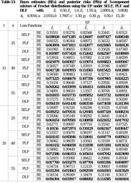
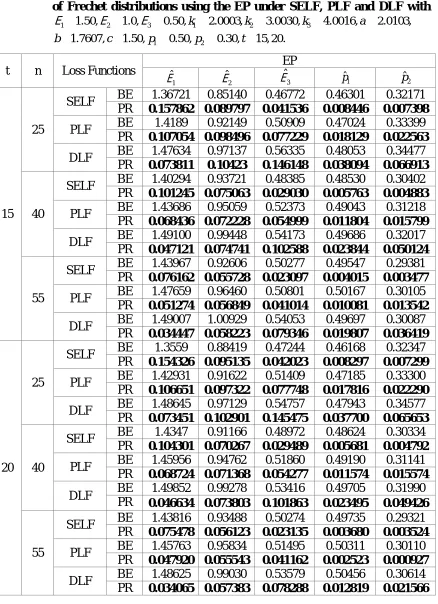
Table 14: Bayes estimates (BEs) and posterior risks (PRs) of 3-component mixture of Frechet distributions using the EP under SELF, PLF and DLF with
1 2 3 1 2 3
1 2
1.50, 1.0, 0.50, 2.0003, 3.0030, 4.0016, 2.0103,
1.7607, 1.50, 0.50, 0.30, 15, 20.
k k k a
b c p p t
t n Loss Functions EP
1
ˆ
ˆ2
3
ˆ
pˆ1 pˆ2
15 25
SELF BE 1.36721 0.85140 0.46772 0.46301 0.32171
PR 0.157862 0.089797 0.041536 0.008446 0.007398
PLF BE 1.4189 0.92149 0.50909 0.47024 0.33399
PR 0.107054 0.098496 0.077229 0.018129 0.022563
DLF BE 1.47634 0.97137 0.56335 0.48053 0.34477
PR 0.073811 0.10423 0.146148 0.038094 0.066913
40
SELF BE 1.40294 0.93721 0.48385 0.48530 0.30402
PR 0.101245 0.075063 0.029030 0.005763 0.004883
PLF BE 1.43686 0.95059 0.52373 0.49043 0.31218
PR 0.068436 0.072228 0.054999 0.011804 0.015799
DLF BE 1.49100 0.99448 0.54173 0.49686 0.32017
PR 0.047121 0.074741 0.102588 0.023844 0.050124
55
SELF BE 1.43967 0.92606 0.50277 0.49547 0.29381
PR 0.076162 0.055728 0.023097 0.004015 0.003477
PLF BE 1.47659 0.96460 0.50801 0.50167 0.30105
PR 0.051274 0.056849 0.041014 0.010081 0.013542
DLF BE 1.49007 1.00929 0.54053 0.49697 0.30087
PR 0.034447 0.058223 0.079346 0.019807 0.036419
20 25
SELF BE 1.3559 0.88419 0.47244 0.46168 0.32347
PR 0.154326 0.095135 0.042023 0.008297 0.007299
PLF BE 1.42931 0.91622 0.51409 0.47185 0.33300
PR 0.106651 0.097322 0.077748 0.017816 0.022290
DLF BE 1.48645 0.97129 0.54757 0.47943 0.34577
PR 0.073451 0.102901 0.145475 0.037700 0.065653
40
SELF BE 1.4347 0.91166 0.48972 0.48624 0.30334
PR 0.104301 0.070267 0.029489 0.005681 0.004792
PLF BE 1.45956 0.94762 0.51860 0.49190 0.31141
PR 0.068724 0.071368 0.054277 0.011574 0.015574
DLF BE 1.49852 0.99278 0.53416 0.49705 0.31990
PR 0.046634 0.073803 0.101863 0.023495 0.049426
55
SELF BE 1.43816 0.93488 0.50274 0.49735 0.29321
PR 0.075478 0.056123 0.023135 0.003680 0.003524
PLF BE 1.45763 0.95834 0.51495 0.50311 0.30110
PR 0.047920 0.055543 0.041162 0.002523 0.000927
DLF BE 1.48625 0.99030 0.53579 0.50456 0.30614
t n Loss Functions ILP
1
ˆ
ˆ2 ˆ3 pˆ1 pˆ2
15 25
SELF BE 0.56523 1.01139 1.12826 0.31465 0.45912
PR 0.044554 0.090911 0.267451 0.008230 0.009621
PLF BE 0.59757 1.04628 1.23254 0.32907 0.46956
PR 0.065972 0.081507 0.211980 0.025600 0.020770
DLF BE 0.63355 1.0946 1.33595 0.34240 0.47914
PR 0.107596 0.076576 0.164423 0.076680 0.044163
40
SELF BE 0.54201 1.00966 1.23515 0.29845 0.48646
PR 0.026295 0.053873 0.208363 0.005167 0.006284
PLF BE 0.57394 1.02998 1.31238 0.30605 0.49318
PR 0.044519 0.049916 0.152275 0.017071 0.012805
DLF BE 0.59161 1.06348 1.40867 0.31462 0.49928
PR 0.076175 0.047963 0.112568 0.055395 0.026073
55
SELF BE 0.53336 1.00855 1.30808 0.28957 0.49727
PR 0.018927 0.038060 0.169564 0.003838 0.004994
PLF BE 0.55034 1.03025 1.38071 0.29622 0.50312
PR 0.032747 0.036346 0.121035 0.015682 0.014800
DLF BE 0.57377 1.04171 1.42649 0.30118 0.50569
PR 0.058687 0.034896 0.085874 0.044595 0.019809
20 25
SELF BE 0.57062 1.00137 1.12997 0.31516 0.45869
PR 0.044086 0.087920 0.263408 0.008132 0.009446
PLF BE 0.59099 1.04844 1.23516 0.32663 0.47035
PR 0.065263 0.080717 0.208417 0.025358 0.020369
DLF BE 0.63333 1.08936 1.32068 0.34144 0.47984
PR 0.10689 0.075730 0.161844 0.075847 0.043153
40
SELF BE 0.54405 1.00478 1.24465 0.29727 0.48533
PR 0.026580 0.053027 0.20577 0.005089 0.006168
PLF BE 0.56536 1.02789 1.33523 0.30662 0.49226
PR 0.043443 0.049528 0.152538 0.016898 0.012658
DLF BE 0.5856 1.05776 1.41234 0.31451 0.49793
PR 0.075514 0.047664 0.110136 0.054559 0.025622
Pak.j.stat.oper.res. Vol.XIII No.3 2017 pp501-528 527
Table 16: Bayes estimates (BEs) and posterior risks (PRs) of 3-component mixture of Frechet distributions using the ILP under SELF, PLF and DLF with
1 1.50, 2 1.0, 3 0.50,a1 1.9520,a2 2.5321,a3 3.7735,a 0.2763,
1 2
0.1167, 1.0, 0.50, 0.30, 15, 20.
b c p p t
t n Loss Functions ILP
1
ˆ
ˆ2
3
ˆ
pˆ1 pˆ2
15 25
SELF BE 1.50074 1.0113 0.52618 0.46474 0.30720
PR 0.201677 0.139007 0.059989 0.009709 0.008305
PLF BE 1.54865 1.07166 0.59254 0.47333 0.32032
PR 0.121795 0.121661 0.097373 0.020884 0.026615
DLF BE 1.60815 1.11961 0.63334 0.48408 0.33550
PR 0.077116 0.109754 0.158355 0.043828 0.081399
40
SELF BE 1.49739 1.00421 0.52511 0.48826 0.29331
PR 0.118952 0.091144 0.0375302 0.006323 0.005249
PLF BE 1.51982 1.06185 0.56073 0.49484 0.30091
PR 0.074183 0.084245 0.062091 0.012935 0.017727
DLF BE 1.55871 1.09042 0.59615 0.50119 0.31088
PR 0.048309 0.077631 0.107985 0.026403 0.058509
55
SELF BE 1.48179 0.99830 0.52107 0.48653 0.27762
PR 0.065501 0.065509 0.026486 0.088606 0.026670
PLF BE 1.50733 1.04203 0.55675 0.50402 0.29269
PR 0.051611 0.062028 0.046765 0.026645 0.023686
DLF BE 1.55419 1.06093 0.56901 0.50656 0.29809
PR 0.035235 0.059862 0.082028 0.020493 0.047445
20 25
SELF BE 1.47373 1.01137 0.53491 0.46469 0.30656
PR 0.190802 0.137987 0.060765 0.009544 0.008152
PLF BE 1.54108 1.05272 0.58151 0.47358 0.32062
PR 0.119934 0.118052 0.094908 0.020467 0.026116
DLF BE 1.61174 1.12454 0.63601 0.48493 0.33430
PR 0.076170 0.1087 0.15734 0.042688 0.080048
40
SELF BE 1.51793 1.00136 0.52995 0.48844 0.29322
PR 0.121567 0.088951 0.038132 0.006279 0.005174
PLF BE 1.53265 1.05414 0.55450 0.49635 0.30019
PR 0.073937 0.082790 0.061166 0.013372 0.017617
DLF BE 1.56394 1.09718 0.59098 0.50066 0.31115
PR 0.047889 0.076504 0.107358 0.025402 0.056618
55
SELF BE 1.49135 1.0110 0.52763 0.49673 0.28394
PR 0.082760 0.068240 0.026867 0.003964 0.003526
PLF BE 1.53327 1.03902 0.54873 0.50575 0.29170
PR 0.053625 0.062574 0.045836 0.015091 0.016591
DLF BE 1.56188 1.06231 0.56084 0.50672 0.29697
1
2 3 1 2
UP
SELF BE 4.40085 3.52976 2.89294 0.25687 0.33460
PR 0.81291 0.398116 0.21769 0.002437 0.002781
PLF BE 4.49226 3.58571 2.93033 0.26157 0.33873
PR 0.182818 0.111902 0.074766 0.009401 0.008261
DLF BE 4.58557 3.64254 2.96819 0.26636 0.34292
PR 0.040282 0.030964 0.025352 0.035618 0.024239
JP
SELF BE 4.22572 3.42494 2.82415 0.25659 0.33463
PR 0.784679 0.387813 0.21316 0.002438 0.002786
PLF BE 4.31757 3.48109 2.86164 0.26130 0.33876
PR 0.183695 0.112312 0.074980 0.009416 0.008273
DLF BE 4.41141 3.53817 2.89963 0.26609 0.34295
PR 0.042093 0.032003 0.026030 0.035712 0.024273
EP
SELF BE 3.29247 2.72831 2.28724 0.26750 0.33895
PR 0.137801 0.086027 0.058819 0.007456 0.006175
PLF BE 3.36137 2.72831 2.28724 0.26750 0.33895
PR 0.137801 0.086027 0.058819 0.007456 0.006175
DLF BE 3.43171 2.77201 2.31703 0.27128 0.34207
PR 0.040575 0.031283 0.025551 0.027679 0.018135
ILP
SELF BE 3.68196 3.06762 2.5327 0.25202 0.33045
PR 0.589974 0.308466 0.16967 0.002605 0.003082
PLF BE 3.76123 3.11749 2.56598 0.25714 0.33508
PR 0.158527 0.099745 0.066555 0.010233 0.009262
DLF BE 3.8422 3.16817 2.5997 0.26236 0.33978