Inverse problems for nonlinear delay systems

Inverse Problems for Nonlinear Delay Systems

Center for Research in Scientific Computation Center for Quantitative Sciences in Biomedicine

North Carolina State University Raleigh, NC 27695-8212

March 15, 2011

Abstract

We consider inverse or parameter estimation problems for general nonlinear nonau-tonomous dynamical systems with delays. The parameters may be from a Euclidean set as usual, may be time dependent coefficients or may be probability distributions across a population as arise in aggregate data problems. Theoretical convergence re-sults for finite dimensional approximations to the systems are given. Several examples are used to illustrate the ideas and computational results that demonstrate efficacy of the approximations are presented.

1

Introduction

Delay differential equations have been a topic of much interest in the mathematical research literature for more than 50 years. Contributions range from classical applications and theo-retical and computational methodologies [Ba79, Ba82, BBu1, BBu2, BKap, BellmanCooke, Cushing, Diekmann, Driver, Gorecki, JKH1, JKH2, JKH3, Kap82, KapSal87, KapSal89, KapSch, Kuang, Minorsky, Webb, Wright] to modern applications in biology [BBJ, BBH, MSNP, NMiP, NMuP, NP]. In this paper we return to a topic that has become increasingly relevant in current research: a theoretical and computational approach for inverse problems involving nonlinear delay systems. One approach that is by now classical dates back to the 1970’s [Ba79, BBu1, BBu2, BKap]. In this approach one approximates solutions to the infinite dimensional state systems such as (1) below by first converting them to an abstract evolution equation in a functional analytic state space setting. One can approximate solu-tions in finite dimensional subspaces spanned by pre-chosen basis elements (e.g., piece-wise linear or cubic splines) in a Galerkin approach which is equivalent to a finite element ap-proximation framework (as is classically used for partial differential equations). One is then able to numerically calculate the generalized Fourier coefficients of approximate solutions relative to the splines, and with these coefficients, recover an approximation to the solutions of delay systems (1).

Here we turn to the mathematical aspects of these nonlinear FDE systems and present an outline of the necessary mathematical and numerical analysis foundations. Thus we provide an extension (to treat time dependent coefficients and general parameters including probability measures) of arguments for approximation and convergence in inverse problems found in [Ba82].

For nonlinear delay systems such as those discussed here, approximation in the context of a linear semigroup framework as presented [BBu1, BBu2, BKap] is not direct. However one can use the ideas of that theory as a basis for a wide class of nonlinear delay system approximations. Details in this direction can be found in the early work [Ba79, Kap82] which is a direct extension of the results of [BBu1, BBu2, BKap] to nonlinear delay sys-tems. The new theoretical results presented here are extensions of these earlier ideas to general nonlinear, nonautonomous delay systems; specifically we extend the ideas of [Ba82] to treat nonlinear systems with time dependent coefficients and/or parameters that may be probabilistic in nature (i.e., probability distributions as treated in [BBoIP, BBPP]). Several current application areas are used to illustrate the theory with examples.

We consider general systems of the form

˙

z(t) =f(t, z(t), zt, z(t−τ1), . . . , z(t−τm), q) +f2(t), 0≤t≤T, z0 =φ (1)

wheref =f(t, η, ψ, y₁, . . . , ym, q) : [0, T]×X×Rnm×Q →Rn. HereX=Rn×L2(−r,0;Rn),

0 < τ₁ < . . . < τm = r, zt denotes the usual function zt(θ) = z(t+θ), −r ≤ θ ≤ 0, and

φ∈H1(−r,0). Here the admissible parameter setQ is a subset of a metric space (possibly infinite dimensional – i.e., some set of functions).

least squares output functional

J(q, d) =

K

i=1

|Cz(ti;q) −di|2, (2)

whereC is an observation operator and{di} is a given data set.

As we shall see below, one can rewrite (1) as

˙

x(t) = A(t, q)x(t) +f(t)

x(0) = x₀, (3)

for states x(t) = (z(t), zt) in an abstract space X. One can then develop theoretical and

computational methodologies to treat finite dimensional approximations in spacesXN and QM_{. These ideas are the focus of our presentation below.}

2

Inverse or Parameter Estimation Problems

2.1 Approximation and Convergence

For more details on general inverse problem methodology in the context of abstract dis-tributed systems, the reader may consult [BK, BSW]. The book [BK] contains a general treatment of inverse problems for partial differential equations in a functional analytic setting. Here we treat nonlinear delay systems with a general family of probabilistic pa-rameters.

The minimization in general abstract parameter estimation problems for (3) involves an infinite dimensional state spaceX and an infinite dimensional admissible parameter set Q (generally of functions or even probability distributions). To obtain computationally tractable methods, we thus consider Galerkin type approximations. Let XN be a sequence of finite dimensional subspaces of X, and QM be a sequence of finite dimensional sets approximating the parameter set Q. We denote by PN the orthogonal projections of X onto XN. Then a family of approximating estimation problems with finite dimensional state spaces and parameter sets can be formulated by seekingq∈ QM which minimizes

JN(q, d) =

K

i=1

|CxN(ti;q)−di|2, (4)

wherexN(t;q)∈XN is the solution to a finite dimensional approximation of (3)) given by

˙

xN_{(t) = A}N_{(t, q)x}N_{(t) +P}N_f(t)

xN(0) = PNx₀. (5)

For the parameter setsQandQM,and state spacesXN,we make the following hypotheses.

(A1M) The sets Q and QM _{lie in a metric space ˜Q with metric d. It is assumed that Q}

and QM are compact in this metric and there is a mapping iM : Q → QM so that QM _=iM_{(Q). Furthermore, for each q ∈ Q, i}M_{(q) → q in ˜Q with the convergence}

(A2N) The finite dimensional subspacesXN satisfy the approximation: For eachx∈X,|x− PNx|X →0 as N → ∞.

Solving the approximate estimation problems involving (4),(5), we obtain a sequence of parameter estimates {q¯N,M}.It is of paramount importance to establish conditions un-der which {q¯N,M} (or some subsequence) converges to a solution for the original infinite dimensional estimation problem involving (2),(3). Toward this goal we have the following results.

Theorem 1. To obtain convergence of at least a subsequence of {q¯N,M} to a solution q¯

of minimizing (4) subject to (5), it suffices, under assumption (A1M), to argue that for arbitrary sequences{qN,M} in QM with qN,M →q in Q,we have

xN(t;qN,M)→x(t;q). (6)

Proof: Under the assumptions (A1M), let{q¯N,M} be solutions minimizing (4) subject to the finite dimensional system (5) and let ˆqN,M ∈ Qbe such thatiM(ˆqN,M) = ¯qN,M.From the compactness of Q,we may select subsequences, again denoted by {qˆN,M} and {q¯N,M}, so that ˆqN,M →q¯∈ Qand ¯qN,M →q¯(the latter follows from the last statement of (A1M)). The optimality of{q¯N,M_{}guarantees that for every q∈ Q}

JN(¯qN,M, d)≤JN(iM(q), d). (7)

Using (6), the last statement of (A1M) and taking the limit asN, M → ∞ in the inequality (7), we obtain J(¯q, d) ≤J(q, d) for every q ∈ Q, or that ¯q is a solution of the problem for (2),(3). We observe that under uniqueness assumptions on the problems (a situation that we hasten to add is not often realized in practice), one can actually guarantee convergence of the entire sequence{q¯N,M} in place of subsequential convergence to solutions.

We note that the essential aspects in the arguments given above involve compactness assumptions on the setsQM andQ.Such compactness ideas play a fundamental role in other theoretical and computational aspects of these problems. For example, one can formulate distinct concepts of problem stability and method stability as in [BK] involving some type of continuous dependence of solutions on the observations z, and use conditions similar to those of (6) and (A1M), with compactness again playing a critical role, to guarantee stability. We illustrate with a simple form ofmethod stability (other stronger forms are also amenable to this approach–see [BK]).

We might say that an approximation method, such as that formulated above involving QM_{, X}N _{and (4)-(5), is stable if}

dist(˜qN,M(dk),q˜(d∗))→0

asN, M, k → ∞ for anydk →d∗ (in this case in the appropriate Euclidean space), where ˜

(i) If {qM} is any sequence with qM ∈ QM, then there exist q∗ in Q and subsequence {qMk}_{with q}Mk →_q∗ _{in the ˜}Q _topology.

(ii) Forany q ∈ Q,there exists a sequence{qM} withqM ∈ QM such thatqM →q in ˜Q.

Similar ideas may be employed to discuss the question of problem stability for the prob-lem of minimizing (2) over Q (i.e., the original problem) and again compactness of the admissible parameter set plays a critical role.

Compactness of parameter sets also plays an important role in computational considera-tions. In certain problems, the formulation outlined above (involvingQM =iM(Q)) results in a computational framework wherein the QM and Q all lie in some uniform set pos-sessing compactness properties. The compactness criteria can then be reduced to uniform constraints on the derivatives of the admissible parameter functions. There are numerical examples (for example, see [BI86]) which demonstrate that imposition of these constraints is necessary (and sufficient) for convergence of the resulting algorithms. (This offers a pos-sible explanation for some of the numerical failures [YY] of such methods reported in the engineering literature.)

The sets (spaces) Q andQM in the inverse problem framework above are an important component in any problem formulation and may involve constant vector parameters, time or spatially dependent functions or even probability measures. In many widely encountered problems the set of admissible parametersQ may consist of simply some compact subset of finite dimensional Euclidean space. In this case one does not need the additional family of sets QM in the above theory (i.e., the above formulation and theory holds with QM = Q for all M). However in an increasing number of applications (for example in the three examples outlined below) the parameters sought are functions of time or space. Then one often uses approximation families to construct the familyQM. For example, in Example 1 below, some of the parameters to be estimated are time dependent coefficients in ordinary differential equation dynamical systems. In this case one might choose some set of functions Q on a time interval [0, T] and then choose piecewise linear splines for the approximating familiesQM (see [BBJ] for details) and use spline approximation properties (e.g., see [BK]) to argue that the conditions of(A1M) hold.

Problems with uncertainty in parameters (or parameters representing some distribu-tion across a populadistribu-tion in the case of aggregate data [BBi, BBH, BBPP, BD, BDTR, BDEHADB, BDEHAD, BFPZ, BG1, BG2, BPi, BPo]) pose even more interesting and challenging possibilities. Several choices may arise for an underlying finite dimensional Eu-clidean set Q: (i) Q is a compact subset of Rp; (ii) Q = [−r,0] is a set of possible delay times τ in some dynamical process. In these cases a frequent choice is

Q=P(Q) ={P :Q→R1 : P is a probability distribution on Q},

i.e., Q is the set of all probability distributions on Q. To investigate theoretical, com-putational and approximation issues for these problems, it is necessary to put a topology on the space of probability measures: a natural choice for P(Q) is the Prohorov met-ric ρ topology (see [Bi, Hu, P]). Convergence in this metric ρ(Pk, P) → 0 is equivalent

to _QgdPk(q) →

QgdP(q) for all bounded, continuous g : Q → R1. Thus if we view

P(Q) ⊂ CB(Q)∗, convergence in the Prohorov metric is equivalent to weak∗ convergence

and the weak∗ topology is metrizable with the Prohorov metric. Then one must construct familiesQM =PM(Q) to approximate the distributionsQ=P(Q) in the Prohorov metric. To pursue this, it is useful to formulate methods to yield finite dimensional setsPM(Q) over which to minimizeJ(P). Of course, we wish to choose these methods so that “PM(Q)→ P(Q)” in some sense so that the conditions(AIM)can be satisfied. This can be done in the context of a framework one based on theProhorov metric[BBPP, BBi] of weak* convergence of measures.

A general theoretical framework is given in [BBPP] with specific results on the approx-imations we use here given in [BBi, BPi]. Briefly, ideas for the underlying theory are as follows:

1. One arguescontinuity of P →J(P) onQ=P(Q) with the Prohorov metricρ;

2. If Q is compact then Q = P(Q) is a complete metric space, indeed compact, when taken with Prohorov metric;

3. Approximation familiesQM =PM(Q) are chosen so that elementsPM ∈ PM(Q) can be found to approximate elements P ∈ P(Q) in Prohorov metric;

4. Well-posedness (existence, continuous dependence of estimates on data, etc.) is ob-tained along with feasible computational methods.

The desired results can be developed using several approximation theories that have been recently developed and used in the context of problems other than those with delay systems. The first, developed in [BBi] and based on Dirac delta measures, is summarized in the following theorem.

Theorem 2. LetQbe a complete, separable metric space, Bthe class of all Borel subsets of

Q and P(Q) the space of probability measures on(Q,B). Let Q₀={qj}∞j=1 be a countable, dense subset of Q. Then the set of P ∈ P(Q) such that P has finite support in Q₀ and rational masses is dense in P(Q) in the ρ metric. That is,

P0(Q)≡ {P ∈ P(Q) :P =

k

j=1

pjΔqj, k∈ N+, qj ∈Q0, pj rational, k

j=1

pj = 1}

is dense inP(Q) taken with the ρ metric, whereΔqj is the Dirac measure with atom atqj.

It is rather easy to use the ideas and results associated with this theorem to develop com-putationally efficient schemes. Given Qd=

_∞

M=1QM withQM ={qMj }Mj=1 (a “partition”

of Q) chosen so thatQd is dense inQ, define

QM _=PM_{(Q) ={P ∈ P(Q) :P =} M

j=1

pjΔqM_j , qjM ∈QM, pj rational, M

j=1

pj = 1}.

Then we find

(ii)PM(Q)⊂ PM+1(Q) whenever QM+1 is a refinement ofQM,

(iii)“PM(Q)→ P(Q)” in theρtopology; that is, forM sufficiently large, elements inP(Q) can be approximated in theρ metric by elements ofPM.

A second class of approximations was developed and used in [BPi] for problems where one assumes that the probability distributions to be approximated possess densities inL2. These involves approximation with piecewise linear splines at the level of the densities.

Theorem 3. Let F be a weakly compact subset of L2(Q), Q compact and let P_F(Q) ≡ {P ∈ P(Q) :P =p, p ∈ F}. Then Q=P_F(Q) is compact inQ˜ =P(Q) in the ρ metric. Moreover, if we define {M_j } to be the linear splines on Q corresponding to the partition

QM, where

MQM is dense in Q, define

PM _{≡ {p}M _:pM ₌ j

bM_j M_j , bM_j rational}

and if

QM _=P

FM ≡ {P_M ∈ P(Q) :P_M =

pM, pM ∈ PM},

we have _MP_FM is dense inQ=P_F(Q) taken with theρ metric.

A study comparing the relative strengths and weaknesses of these two classes of approx-imation schemes in the context of inverse problems is given in [BD].

Thus we have that compactness of admissible parameter sets play a fundamental role in a number of aspects, both theoretical and computational, in parameter estimation problems. This compactness may be assumed (and imposed) explicitly as we have outlined here, or it may be included implicitly in the problem formulation throughTikhonov regularization as discussed for example by Kravaris and Seinfeld [KS], Vogel [Vog] and widely by many others. In the regularization approach one restricts consideration to a subset Q₁ of parameters which has compact embedding in Q and modifies the least-squares criterion to include a term which insures that minimizing sequences will be Q₁ bounded and hence compact in the original parameter setQ.

After this short digression on general inverse problem concepts, we return to the con-vergence (6).

2.2 State Approximation and Convergence for Nonlinear Systems

We consider the general system

˙

z(t) =f(t, z(t), zt, z(t−τ1), . . . , z(t−τm), q) +f2(t), 0≤t≤T, z0 =φ (8)

wheref =f(t, η, ψ, y₁, . . . , ym, q) : [0, T]×X×Rnm×Q →Rn. HereX=Rn×L2(−r,0;Rn),

0 < τ₁ < . . . < τm = r, zt denotes the function zt(θ) = z(t+θ), −r ≤ θ ≤ 0, and

(H1) The function f satisfies a global Lipschitz condition:

|f(t, η, ψ, y₁, . . . , ym, q) − f(t, ξ,ψ, w˜ 1, . . . , wm, q)| ≤

K

|η−ξ|+|ψ−ψ˜|+m_i=1|yi−wi|

for some fixed constant K and all (η, ψ, y₁, . . . , ym), (ξ,ψ, w˜ 1, . . . , wm) in X×Rnm

uniformly int and in q∈ Q.

(H2) The function f(·,··, q) : [0, T]×X×Rnm→Rn is differentiable for each q.

(H3) The function q→f(·,··, q) is continuous on Q.

Remark 1. If we define the functionF : [0, T]×Rn×C(−r,0;Rn)×Q ⊂[0, T]×X×Q →Rn given by

F(t, x, q) =F(t, η, ψ, q) =f(t, η, ψ, ψ(−τ₁), . . . , ψ(−τm), q) (9)

we observe that even though f satisfies (H1),F will not satisfy a continuity hypothesis on its domain in theX norm.

We define the nonlinear operator A(t;q) :D(A)⊂X→X by

D(A)≡ {(ψ(0), ψ)|ψ∈H1(−r,0)}

A(t;q)(ψ(0), ψ) ≡(F(t, ψ(0), ψ, q), Dψ)

where here Dψ =ψ. Note that D(A) is independent of t and q. We then may write the system (8) in abstract form

˙

x(t) = A(t;q)x(t) + (f₂(t),0)

x(0) = ζ = (φ(0), φ), (10)

for statesx(t) = (z(t), zt) in the abstract spaceX.

Theorem 4. Assume that (H1) holds and let x(t;φ, f₂) = (z(t;φ, f₂), zt(φ, f2)), where z is the solution of (8) corresponding to φ∈H1, f₂ ∈L₂. Then for ζ = (φ(0), φ), x(t;φ, f₂) is the unique solution on [0, T]of

x(t;q) =ζ+

t

0 [A(σ;q)x(σ;q) + (f2(σ),0)]dσ. (11)

Furthermore,f₂ →x(t;φ, f₂)is weakly sequentially continuous fromL₂ (weak) toX(strong).

The uniqueness of solutions to (11) follows in the usual manner once we establish that Asatisfies a dissipative inequality. We do this in a spaceXg that is topologically equivalent

to X. Renorm X by the weighting function g defined on [−r,0), where g(ξ) = j for ξ ∈ [−τm−j+1,−τm−j), j = 1,2, . . . , m (we define τ0 = 0). Define the Hilbert space Xg ≡

Rn_×L

2(−r,0;g;Rn) to be the elements of X with this new inner product

<(η, φ),(ζ, ψ)>Xg=< η, ζ >Rn +

₀

−r

φ(ξ)ψ(ξ)g(ξ)dξ. (12)

This gives rise to an equivalent topology to that ofX as long asg(ξ)>0 for all ξ∈[−r,0) (see [BBu2, p. 186], [BKap, Webb] for more details). Then the nonlinear operator A(t;q) is dissipative if for someκ >0 we have

A(t;q)x− A(t;q)w, x−w Xg ≤κx−w, x−w Xg (13)

for allx, w∈ D(A) and alltand q∈ Q. This can be used to immediately argue uniqueness of solutions. We outline the arguments to establish the fundamental inequality (13). We have for x= (φ(0), φ), w= (ψ(0), ψ)

<A(t;q)x− A(t;q)w, x−w >Xg = < F(t, φ(0), φ)−F(t, ψ(0), ψ), φ(0)−ψ(0)>Rn

+< Dφ−Dψ, φ−ψ >_{L2(−r,0;g;R}n₎

= < F(t, φ(0), φ)−F(t, ψ(0), ψ), φ(0)−ψ(0)>_Rn

+

₀

−r

D(φ(ξ)−ψ(ξ))(φ(ξ)−ψ(ξ))g(ξ)dξ

= < F(t, φ(0), φ)−F(t, ψ(0), ψ), φ(0)−ψ(0)>_Rn

+

m

j=1

₋τm−j

−τm−j+1

D(φ(ξ)−ψ(ξ))(φ(ξ)−ψ(ξ))g(ξ)dξ.

(14)

Consider the last term and denote Δm−j = (φ−ψ)(τm−j) = φ(−τm−j)−ψ(−τm−j) for

m

j=1

₋τm−j

−τm−j+1

D(Δ(ξ))Δ(ξ)g(ξ)dξ

=

m

j=1

1 2jΔ(ξ)

2_|ξ=−τm−j

ξ=−τm−j+1

=

m

j=1

j

2|Δm−j|

2₋j

2|Δm−j+1|

2 = 1 2 m j=1

j|Δm−j|2−

1 2

m−1

k=0

(k+ 1)|Δm−k|2 ( for k=j−1)

= 1 2m|Δ0|

2₊1

2

m−1

j=1

j|Δm−j|2−

1 2

m−1

k=1

(k+ 1)|Δm−k|2−

1 2|Δm|

2

= 1 2m|Δ0|

2₋1

2

m−1

j=1

|Δm−j|2−

1 2|Δm|

2

= 1 2m|Δ0|

2₋1

2

m−1

j=0

|Δm−j|2=

m+ 1 2 |Δ0|

2₋1

2

m

j=0

|Δm−j|2

Returning to (14), we have

<A(t;q)x− A(t;q)w, x−w >Xg ≤ |< F(t, φ(0), φ)−F(t, ψ(0), ψ), φ(0)−ψ(0)>Rn |

+m+ 1 2 |Δ0|

2₋1

2

m

j=0

|Δm−j|2

≤ K

|Δ₀|+|Δ|+

m

i=1

|Δi|

|Δ₀|

+m+ 1 2 |Δ0|

2₋1

2

m

j=0

|Δm−j|2

≤ K|Δ₀|2+ K

2

2 |Δ|

2₊1

2|Δ0|

2₊1

2

m

i=1

|Δi|2+

mK2 2 |Δ0|

2

+m+ 1 2 |Δ0|

2₋1

2

m

j=0

|Δm−j|2

≤ K+mK

2

2 +

m+ 1 2

|Δ0|2+ K

2

2 |Δ|

2 L2

≤ K+mK

2

2 +

m+ 1 2

|Δ|2_X

using the definition of the inner product. Therefore choosing

κ=K+mK2

2 +

m+ 1 2 , we have thatA(t;q) is dissipative inXg, uniformly in tand q .

Turning next to the approximation of (8) through approximation of (11), we letXN be the spline subspaces of X discussed in detail in [BKap]. We briefly outline the results for the piecewise linear subspacesX₁N (see Section 4 of [BKap]) given by

X₁N ={(φ(0), φ)| φis a continuous first-order spline function with knots attN_j =−jr/N, j= 0,1, . . . , N}.

A careful study of the arguments behind our presentation reveals that the approximation results given here hold for general spline approximations. For example, if one were to treat cubic spline approximations (X₃N of [BKap]), one would use the appropriate approximation analogues of Theorem 2.5 of [Schultz] and Theorem 21 of [SchuVarg] (e.g., see Theorem 4.5 of [Schultz]). Hereafter, when we write XN, the reader should understand that we mean X₁N of [BKap].

LetPN =P_gN be the orthogonal projection (in, g ≡ , Xg) of X ontoXN so that as

we have already discussed it immediately follows that PNx→ x for all x∈ X. Similar to the approach in [BKap] as extended in [Ba82], for arbitrary {qN} with qN → q we define the approximating operator

AN_{(t) =P}N_A(t;qN_)PN

and consider the approximating equations inXN given by

xN(t) =PNζ+

t

0 [A

N_(σ)xN_{(σ) +P}N_(f

2(σ),0)]dσ (15)

which, becauseXN is finite-dimensional, are equivalent to

˙

xN(t) =AN(t)xN(t) +PN(f₂(t),0), xN(0) =PNζ. (16)

Note that xN(t) = xN(t;QN). From (13) and the definition of AN in terms of the self-adjoint projectionsPN_{, we have at once that under (H1) the sequence {A}N_{}satisfies onX}

a uniform dissipative inequality

AN_{(t)x− A}N_{(t)w, x−w}

g ≤κx−w, x−w g. (17)

Uniqueness of solutions of (15) then follows immediately from this inequality. Upon recog-nition that (16) is equivalent to a nonlinear ordinary differential equation in Euclidean space with the right-hand side satisfying a global Lipschitz condition, one can easily argue exis-tence of solutions for (16) and hence for (15) on any finite interval [0, T]. Our main result to be discussed here, which ensures that solutions of (16) converge to those of (8), can now be stated.

Theorem 5. Assume (H1), (H2), (H3) and qN _{→ q in Q. Let ζ = (φ(0), φ), φ∈H}1 _and

f₂ ∈ L₂(0, T) be given, with xN and x the corresponding solutions on [0, T] of (16) and

(8), respectively. ThenxN(t)→x(t) = (z(t;φ, f₂), zt(φ, f2)), asN → ∞, uniformly in ton

Remark 2. One can actually obtain slightly stronger results than those given in Theorem 5. One can consider solutions of (8) and (16) corresponding to initial data (z(0), z₀) = (η, φ) = ζ with η ∈ Rn, φ∈ L₂ (i.e., ζ ∈X) and argue that the results of Theorem 5 hold also in this case.

To indicate briefly our arguments for Theorem 5, we consider for given initial data ζ and perturbation f₂ the corresponding solutions x and xN of (11) and (15). Define ΔN(t)≡xN(t)−x(t) andF₂(t) = (f₂(t),0), we obtain immediately that

ΔN(t) = (PN −I)ζ+

t

0

AN_(σ)xN_{(σ)− A(σ)x(σ) + (P}N_−I)F

2(σ)dσ. (18)

We next use a rather standard technique for analysis of differential equations (see [Barbu]), the foundations of which we state as a lemma since we shall refer to it again.

Lemma 3. If X is a Hilbert space and x: [a, b]→X is given by

x(t) =x(a) +

t

a

y(σ)dσ,

then

|x(t)|2 =|x(a)|2+ 2

t

0 x(σ), y(σ) dσ.

This lemma is essentially a restatement of the well-known result [Barbu, p. 100] that in a Hilbert space

d dt

1 2|x(t)|

2_{=x˙(t), x(t) .}

Applying Lemma 3 to (18), we obtain

|ΔN(t)|2 = |(PN −I)ζ|2

+2₀tAN(σ)xN(σ)− A(σ)x(σ) + (PN −I)F₂(σ),ΔN(σ) dσ

= |(PN −I)ζ|2+ 2₀tAN(σ)xN(σ)− AN(σ)x(σ),ΔN(σ) dσ

If we use (17) on the first integral term in this last expression, we then have

|ΔN(t)|2 ≤ |(PN −I)ζ|2+ 2₀tω|ΔN(σ)|2dσ

+2₀t(AN(σ)− A(σ))x(σ) + (PN −I)F₂(σ),ΔN(σ) dσ

≤ |(PN −I)ζ|2+ 2₀tω|ΔN(σ)|2dσ

+2₀t[1₂|(AN(σ)− A(σ))x(σ)|2+₂1|ΔN(σ)|2

+1₂(PN −I)F₂(σ)2+1₂ΔN(σ)2]dσ

= (PN _−I)ζ2₊t

0(AN(σ)− A(σ))x(σ)2dσ+

t

0 (PN −I)F2(σ)2dσ

+2(ω+ 1)₀t|ΔN_(σ)|2_dσ.

An application of Gronwall’s inequality to this then yields the estimate

|ΔN(t)|2 ≤[₁(N) +₂(N) +₃(N)] exp (2(ω+ 1)t), (19)

where

₁(N) =|(PN−I)ζ|2,

₂(N) =

T

0

(AN(σ)− A(σ))x(σ)2dσ,

₃(N) =

T

0

_(PN _−I)F

2(σ)2dσ.

Since PN →I strongly inX and the convergence |(PN −I)F₂(σ)| →0 in₃ is dominated, to prove Theorem 5 it suffices to argue that ₂(N)→ 0 as N → ∞. To that end, we state the following sequence of lemmas.

Lemma 4. Assume (H1), (H3) and let X ≡ {x = (φ(0), φ) | φ∈ H2}. Then for each t,

AN_{(t)x→ A(t)x as N → ∞ for each x∈ X.}

Lemma 5. For fixed q ∈ Q, let Cq ≡ {(ζ, f2) ∈ D(A)×L2(0, T) |φ ∈H2, f2 ∈ H1, with

˙

φ(0) = F(0, ζ, q) +f₂(0) where ζ = (φ(0), φ)}. Assume that (H1), (H2) hold. Then for

(ζ, f₂) ∈ Cq the corresponding solution σ → x(σ) = (z(σ), zσ) of (11) (z is the solution of

(8)) satisfies x(σ)∈ X for each σ∈(0, T].

Lemma 6. Assume (H1), (H2), (H3) and let(ζ, f₂)∈ Cq with xN and x the corresponding solutions of (15) and (11). Then xN(t)→x(t) uniformly in t on [0, T].

Lemma 7. Assume (H1). Then the solutions of (11)and (15)depend continuously (in the

X×L₂ topology) on (ζ, f₂)∈ D(A)×L₂, uniformly in t on [0, T].

We obtain the convergence of Theorem 5 by combining Lemmas 6, 7 and 8. The proof of Lemma 7 employs Lemma 3 along with Gronwall’s inequality in much the same way as above in deriving (19) from (18). We note that Lemma 5 requires hypothesis (H2) in order to obtain enough smoothness of solutionsx of (11) so thatx(σ)∈ X for eachσ, which then permits the convergence arguments of Lemma 6.

In developing the estimates to establish Lemma 6 (which, by our above remarks, requires only that we argue ₂(N) → 0), we use heavily the standard spline estimates found in [Schultz] and [SchuVarg]. Lemmas 4 and 5 yield that AN(σ)x(σ) → A(σ)x(σ) for each σ so that to prove Lemma 6 one only need show that this convergence is dominated, thereby guaranteeing ₂(N) → 0. In making the arguments for Lemma 6, one obtains at the same time error estimates on the convergence in Theorem 5. For example, one readily finds the following: forφ∈H2,f satisfying (H1), (H2), ˙φ(0) =F(φ(0), φ) and f₂≡0, the convergencexN(t)→x(t) isO(1/N). For higher-order splines and higher-order convergence estimates (e.g., cubic splines with convergence O(1/N3)), one of course needs additional smoothness (beyond (H2)) on f.

The convergence given in Theorem 5 yields state approximation techniques for nonlinear FDE systems based on the spline methods developed in [BKap]. These results can be applied directly to control and identification problems, the latter of which are discussed in [Ba82].

Remark 9. Results for special classes of the systems above can actually be obtained from the arguments for nonautonomous nonlinear delay systems in [Ba79]. In that approach, one requires all discrete delays to appear in the linear part of the system dynamics while continuous delays may appear in the nonlinear part. One then writes the system dynamics as an autonomous linear part plus a nonlinear perturbation. The linear part generates a linear semigroup as in [BBu1, BBu2, BKap]. One then uses the linear semigroup in a vari-ation of parameters implicit representvari-ation of the solution to the nonlinear system. Math-ematical tools used then are Picard iterates for existence, and the Trotter-Kato theorem [BBu1, BBu2, BKap] (for the linear semigroup) plus a Gronwall inequality. An alternative (and more general) approach given in [Ba82] eschews use of the Trotter-Kato theorem in treating general nonautonomous nonlinear delay systems which allows discrete delays in the nonlinear components of the system. As we have seen, the main mathematical tools are dissipative properties of the general nonlinear operator A(t) representing the system and direct approximation AN(t) → A(t) (no Trotter-Kato!) along with a Gronwall inequality. Finally, a nonlinear semigroup (with dissipative generators) approach along with a corre-sponding nonlinear Trotter-Kato convergence result are given by Kappel in [Kap82]. With these results one can treat directly general autonomous nonlinear delay systems in the spirit of a linear semigroup approach [Pa].

3

Examples

above theory in a little more detail for this application and present some specific new and preliminary findings.

3.1 Example 1: Insect/Insecticide Models

We describe here a non-autonomous delay system arising in insect/insecticide investigations [BBDS2, BBJ]. Mathematical models that are suitable for field data with mixed popula-tions should consider reproductive effects and should also account for multiple generapopula-tions, containing neonates (juveniles) and adults and their interconnectedness. This suggests the need at the minimum for a coupled system of equations describing two separate age classes. Additionally, due to individual differences within the insect population, it is biologically un-realistic to assume that all neonate aphids born on the same day reach the adult age class at the same time. In fact, the age at which the insects reach adulthood varies from as few as five to as many as seven days. Hence one must include a term in any model to account for this variability, leading one to develop a coupled differential equation model including distributed delays for the insect population dynamics. We consider the delay between birth and adulthood for neonate pea aphids and present a mathematical model that treats this delay as a random variable.

Let a(t) and n(t) denote the number of adults and neonates, respectively, in the popu-lation at timet. We lump the mortality due to insecticide into one time varying parameter pa(t) for the adults, pn(t) for the neonates, and denote by da(t) anddn(t) the background

or natural mortalities for adults and neonates, respectively. We letb(t) be the time varying rate at which neonates are born into the population.

We suppose that there is a time delay for maturation of a neonate to adult life stage. We further assume that this time delay varies across the insect population according to a probability distribution P(τ) for τ ∈ [−Tn,0] with corresponding density k(τ) = dP_dτ(τ).

Here we tacitly assume an upper bound onTn for the maturation period of neonates into

adults. Thus, we have thatk(τ),τ <0, is the probability per unit time that a neonate who has been in the population −τ time units becomes an adult. Then the rate at which such neonates become adults isn(t+τ)k(τ). Summing over all suchτ’s, we obtain that the rate at which neonates become adults is ₋0_Tnn(t+τ)k(τ)dτ. Using the biological knowledge that the maturation process varies between five and seven days (i.e., k vanishes outside [−7,−5]), we obtain the functional differential equation (FDE) system

da dt(t) =

₋₅

−7 n(t+τ)k(τ)dτ−(da(t) +pa(t))a(t) dn

dt(t) = b(t)a(t)−(dn(t) +pn(t))n(t)−

₋₅

−7 n(t+τ)k(τ)dτ

a(θ) = Φ(θ), n(θ) = Ψ(θ), θ∈[−7,0) a(0) = a0, n(0) =n0,

(20)

wherekis now a probability density kernel which we have assumed has the propertyk(τ)≥0 forτ ∈[−7,−5] andk(τ) = 0 for τ ∈(−∞,−7)∪(−5,0].

In this problem the parameters to be estimated are time dependent coefficients da(t), pa(t), b(t), dn(t), pn(t) as well as the probability density maturation kernels k(τ).

includes these models as special cases of a class of abstract differential equations with function space parameters (including probability densities) which are readily approximated by finite element systems (the spaces QM are piecewise linear splines for time varying coefficients as well as density kernels). The inverse problems are formulated in the context of both ordinary and generalized least squares frameworks, and computations are carried out (including an uncertainty analysis with confidence intervals via asymptotic error analysis involving approximate sampling distributions) with simulated noisy data to demonstrate both efficiency and efficacy of the methodologies.

3.2 Example 2: HIV Infection Dynamics

We next consider classes of nonlinear functional or delay differential equation models which arise in attempts to describe temporal delays in HIV pathogenesis. These models, first developed in [BBH] consider incorporation of variability (i.e., general probability distribu-tions) for these delays into systems that cannot readily be reduced to a finite number of coupled ordinary differential equations (as is done in the method of stages). In [BBH], the authors introduced several classes of nonlinear models (including discrete and distributed delays), and presented discussions of theoretical and computational approaches. The models were validated with in vitroexperimental data [RWE] in successful inverse problem efforts. This was supported by statistical significance tests for the importance of including delays in the dynamics.

The underlying biology is discussed in some detail in [BBH] to which we refer interested readers. Viruses are obligate intra-cellular parasites with a multitude of pathways for infect-ing and reproducinfect-ing within their target hosts. The Human Immunodeficiency Virus (HIV) is a lentivirus that is the etiological agent for the slow, progressive, and fatal Acquired Immunodeficiency Syndrome (AIDS) for which there is currently no known cure.

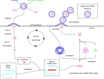
For HIV, the core of the virus is composed of single-stranded viral RNA and protein components. As depicted in Figure 1, when an HIV virion comes into contact with an uninfected CD4 target cell, the viral envelope glycoproteins fuse to the cell’s lipid bilayer at a CD4 receptor site and the viral core is injected into the cell. Once inside, the protein components enable transcription and integration of the viral RNA into viral DNA and then incorporation into the cellular DNA (provirus). With its altered cellular DNA, the cell produces capsids and protein envelopes and transcribes multiple copies of viral RNA. The cell assembles a virion by then encasing the newly produced viral RNA in a capsid followed by a protein envelope. The new HIV virion pushes out through the cell membrane budding off in chains of virions (though sometimes single virions do float away into the plasma). The time from viral infection to viral production (sometimes called the eclipse phase) is not instantaneous, and (as indicated in the figure) it is estimated that the first viral release occurs approximately 24 hours after the initial infection.

reverse transcriptase

RNA capsid

envelope

single-strand RNA lentivirus

infection

cell membrane

cytosol loss of

envelope

loss of

viral capsid

cellular DNA

viral DNA

altered cellular DNA

integration

transcription into multiple RNA copies translation

translation assembly

viral budding

24 hour

mean delay

it is possible for the cells to continue to divide (albeit at a much slower rate than acutely infected or non-infected cells) and to produce virions.

In the course of developing the models, one employs a delay to mathematically represent the temporal lag between the initial viral infection and the first release of new virions. We concentrate on the mathematical modeling of viral dynamics, focusing in particular on the mathematical aspects and biological nature of the delays in primary infection. The models are extensions of previous modeling work on HIV infection dynamics forin vitrolaboratory experiments from the (continuous) delay differential equations developed in [BGHKNS], which in turn were based on a discrete dynamical system from [HE]. Our primary interest here is to present the functional differential equations required when treating cellular level data containing significant variability as a specific example to which the theory developed in this paper is applicable. In this example, a major part of the efforts involved estimation of parameters that are probability densities.

A central focus of the modeling efforts have been on attempting to obtain reasonable mathematical representations of these delays. The problem of how to mathematically repre-sent these phenomena is decidedly nontrivial and includes issues such as how to account for intra-individual variability (e.g., intercellular variability arising within a single infected in-dividual or laboratory assay) and/or inter-inin-dividual variability arising between inin-dividual subjects or data from multiple assays. These issues are highly significant and dealing with the levels of variability and the resulting mathematical ramifications is of primary interest.

The basic model involving delays has the form

˙

V(t) = −cV(t) +nAA(t−τ1) +nCC(t)−pV(t)T(t)

˙

A(t) = (rv−δA−δX(t))A(t)−γA(t−τ1−τ2) +pV(t)T(t)

˙

C(t) = (rv−δC−δX(t))C(t) +γA(t−τ1−τ2)

˙

T(t) = (ru−δu−δX(t)−pV(t))T(t) +S ,

(21)

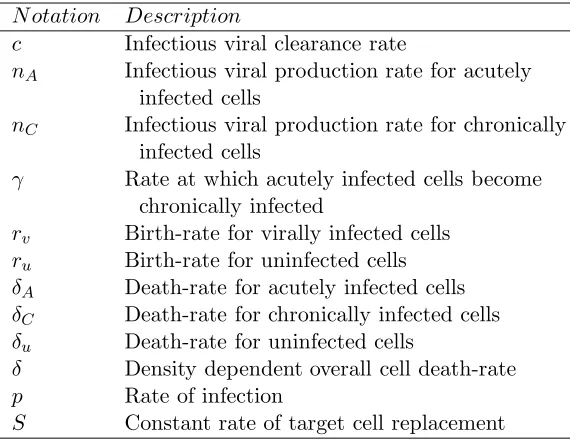
where the state variables are given by V =infectious viral population, A=acutely infected cells, C=chronically infected cells, T=uninfected or target cells, X = A+C+T=total cell population (infected and uninfected), and the parameters are given in Table 1. In this model, it is assumed that the delaysτ₁,τ₂ are fixed for each cell, and that one can precisely describe the capacity of each member of the population (of infected cells) to produce virions as a function of time. More precisely, exactly τ₁ units of time after a cell becomes infected, it begins producing virus. Exactly τ₂ units of time later, that same cell then becomes chronically infected (assuming it lives to this stage).

From a biological viewpoint, it is unlikely that all cells have precisely the same delay times in their production characteristics or conversion to a chronically infected stage. To accommodate some variability expected in such biological populations, let the delay in the first equation in (21) be modeled by treating the delay time τ between acute infection and viral production as a probabilistic quantity (i.e., a random variable) with distributionP₁(τ) so that the first equation in (21) is replaced by (see the appendix of [BBH] for a more detailed discussion of the foundations underlying such an equation)

˙

V(t) =−cV(t) +nA

₀

N otation Description

c Infectious viral clearance rate

nA Infectious viral production rate for acutely

infected cells

nC Infectious viral production rate for chronically

infected cells

γ Rate at which acutely infected cells become chronically infected

rv Birth-rate for virally infected cells

ru Birth-rate for uninfected cells

δA Death-rate for acutely infected cells

δC Death-rate for chronically infected cells

δu Death-rate for uninfected cells

δ Density dependent overall cell death-rate p Rate of infection

S Constant rate of target cell replacement

Table 1: in vitro model parameters

The functionp(V, T), where x→p(x), x= (V, T), is globally Lipschitz as hypothesized in (H1) in Section 2 above. For the efforts here and in [BBH], the functionpis assumed to be locally bilinear, i.e., p(V, T) =pV T before saturation and constant or linear thereafter (see [BBH]).

Likewise, let the delay between acute infectivity and chronic infectivity (with distri-bution P₂(τ)) be represented in altered forms of the second and third equations of (21) by

˙

A(t) = (rv−δA−δX(t))A(t)−γ

₀

−∞A(t+τ)dP2(τ) +pV(t)T(t) (23)

˙

C(t) = (rv−δC−δX(t))C(t) +γ

₀

−∞A(t+τ)dP2(τ). (24)

The resulting model becomes the special case

˙

V(t) = −cV(t) +nA

₀

−∞A(t+τ)k1(τ)dτ+nCC(t)−pV(t)T(t)

˙

A(t) = (rv−δA−δX(t))A(t)−γ

₀

−∞A(t+τ)k2(τ)dτ +pV(t)T(t)

˙

C(t) = (rv−δC−δX(t))C(t) +γ

₀

−∞A(t+τ)k2(τ)dτ

˙

T(t) = (ru−δu−δX(t)−pV(t))T(t) +S ,

(25)

whether or not it should be modeled as a fixed value for every cell or distributed across the cell populations and how this distribution can be represented, as well as further evidence of the statistical significance of the presence of the delays are the focus of discussions in [BBH].

The variablesV andCin the above model are actually expected values. To explain this, we first consider the delay between initial acute infection and initial chronic infection of a cell. It is biologically unrealistic to expect an entire population of cells to simultaneously change infection characteristics ¯μ₂ = τ₁ +τ₂ (¯μ₂ >0) hours after initial viral infection. Therefore, suppose that the delay between initial acute infection and chronic infection varies across the cell population (thus mathematically characterizing the intercellular variability) according to a probabilistic distribution ¯P₂ with density ¯k₂. We denote by C(t;τ) the subpopulation consisting of chronically infected cells that either maintained their acute infection characteristics for τ time units or are the progeny of those same cells. In other words, for someτ >0, there exists a subpopulation C(t;τ) of the chronically infected cells which either spentτ hours as acutely infected cells (before converting to chronically infected cells) or are descendants of cells that spent exactly τ hours as acutely infected cells. Thus, as derived carefully in [BBH] one has

C(t) = E₂[C(t;τ)] = ₀∞C(t;τ)¯k₂(τ)dτ , (26)

where

˙

C(t;τ) = (rv−δC −δX(t))C(t;τ) +γA(t−τ) ,

with

X(t) =A(t) +C(t) +T(t).

Integration of this equation over the distribution ¯P₂, over all possible delays, yields the equation for C, the expected value of the population of chronic cells, given by

˙

C(t) = E₂[ ˙C(t;τ)]

= (rv−δC−δX(t))C(t) +γ

_∞

0 A(t−τ) ¯k2(τ)dτ

C(0) = C₀,

(27)

whereC₀ is the initial condition for the total chronically infected cell population. A simple change of variables in the integral term as described below results in the third equation of (25).

A similar argument can be made for the delay between viral infection and viral pro-duction for the acutely infected cellsA(t). One supposes that the delay between infection and production (for acutely infected cells A(t)) varies across the population with proba-bility distribution ¯P₁ and corresponding density ¯k₁ and partitions the expected total viral populationV into those virions VA produced by acutely infected cells and those virionsVC

produced by chronically infected cells. We then denote by VA(t;τ) the subpopulation of

virus which are produced by an acutely infected cellτ hours after being infected. Thus, the rate of change in this subgroup of virions is governed by

˙

To obtain the (expected) number of virus at time t that have been produced by acutely infected cells, we must integrate over the distribution ¯P₁, over all possible delays

VA(t) =E1[VA(t;τ)] =

_∞

0 VA(t;τ)¯k1(τ)dτ ,

which yields the governing equation for this larger subpopulation of virions

˙

VA(t) = E1[ ˙VA(t;τ)]

= −cVA(t) +nA

_∞

0 A(t−τ)¯k1(τ)dτ−pVA(t)T(t).

To account for the chronically infected cells as a source of virions, we denoteVC as the

sub-population of virions produced by chronically infected cells. Thus the equation describing the rate of change in the size of this subpopulation is

˙

VC(t) = −cVC(t) +nCC(t)−pVC(t)T(t),

where the expected valueC of the total population of chronically infected cells is defined in (26). Therefore, the governing equations for the total population of virus are described by

˙

V(t) = E₁[ ˙VA(t;τ) + ˙VC(t)]

= −c(VA(t) +VC(t)) +nA

_∞

0 A(t−τ)¯k1(τ)dτ +nCC(t)

−p(VA(t) +VC(t))T(t)

= −cV(t) +nA

_∞

0 A(t−τ)¯k1(τ)dτ +nCC(t)−pV(t)T(t)

V(0) = V₀,

whereV₀ is the initial condition for the total virions population.

If one assumes that theA and T subclasses have no subpopulation structures, and are therefore governed by

˙

A(t) = (rv−δA−δX(t))A(t)−γ

_∞

0 A(t−τ) ¯k2(τ)dτ

+pV (t)T(t)

A(0) = A₀ ˙

T(t) = (ru−δu−δX(t)−pV (t))T(t) +S

T(0) = T₀,

with initial conditions A₀ and T₀, we are subsequently led to the model equations (25) by making the change of variables ki(ξ) = ¯ki(−ξ) so that the densities are now defined on

(−∞,0) instead of (0,∞) .

(statistical significance in improving fits-to-data) in the models; (iii) analysis to show that the models with discrete delays yield essentially similar dynamic responses to those from models with continuous delays. This last finding is important biologically since it is highly unlikely that all cells in a population can respond with fixed uniform delays.

3.3 Example 3: The drinking behavior control system (DBCS)

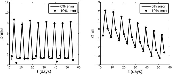
Researchers studying alcohol abuse and addiction have collected vast amounts of information on substance use, participant’s willingness to change behavior, and participant’s success in a particular treatment. Many hypotheses have been formulated concerning possible (difficult-to-measure) factors that control a patient’s motivations and behavior, such as the relative importance of drinking in their lives, commitment to reducing their alcohol consumption, and recognition of reasons to not use a substance, to name a few. However, the relative contributions of these possible mechanisms for behavior change are unclear. The interplay among these factors as they change over time is a natural, albeit difficult, question to address via dynamical mathematical models. In order to better understand these ideas in a quantitative context and to identify underlying mechanisms governing drinking behavior in problem drinkers during therapy, we have, in joint efforts [BRSDHKM] with a team of psychologists at Columbia University, attempted to model behavior control systems informed by a dataset, Project MOTION. We present here an initial model developed in these collaborations.

Further details on Project MOTION and the data collected can be found in [BRSDHKM]. Briefly, approximately 90 participants were assigned to one of three therapy-based treat-ment groups. In addition to attending the four therapy sessions over an eight week period, patients were directed to call an interactive voice recording (IVR) system and answer a survey of 41 questions every day during the evening for eight weeks. Our modeling efforts focused on the data from the IVR surveys since there are numerous longitudinal time points, which we anticipated would be more informative of the underlying dynamic processes.

The 41 questions of the IVR are divided into topical groups in the survey form. Each group has its own scale by which a participants’ numerical responses are interpreted. Since it is prohibitive to construct an initial model from so many variables, we averaged responses from similar categories which led toconceptual variables. Among the conceptual variables we considered based on the IVR data were stressful events, pleasant events, pressure to drink, current mood, perceived stress, desire to drink, commitment to not drink for the next 24 hours, confidence and commitment to reduce drinking for the next 24 hours, guilt concerning drinking behavior, and alcohol consumption. The models were then developed based on these variables. During the formulation of these models based on the longitudinal data, we determined that delays and cumulative effects are important and should be included in order to accurately reflect the dynamic changes in a person’s behavior.

with a statement on the intensity of their feelings on a particular subject. One preliminary simplified model had the form

d

dtA(t) = −a12

0

−r

G(t+s)κ₁(s)ds

2

+a₁₃χ_{D>0}D(t)

d

dtG(t) = a21(A(t−τ1)−A

∗

G) (28)

d

dtD(t) = −a32

exp 1

G∗_D1

₀

−r

G(t+s)κ₂(s)ds

−G∗_D2

,

where κ₁(s) = x+2₂ , κ₂(s) = (x+2)₄ 3, and r = 2, indicating that behavior over the past two days has an impact on current behavior. We included an indicator function χ_(D>0) to reflect that only when a person desires alcohol does his/her drinking behavior change. Additionally, we enforced the conditions A(t) ≥0 and G(t) ≥ 0, where for all variables a value of 0 indicates a neutral value (the scaled variables had values in the range [−2,2]). For example D(t) = 0 indicates neither a desire nor a dislike for alcohol, and G(t) = 0 indicates that a person feels no particular feelings of guilt or virtue.

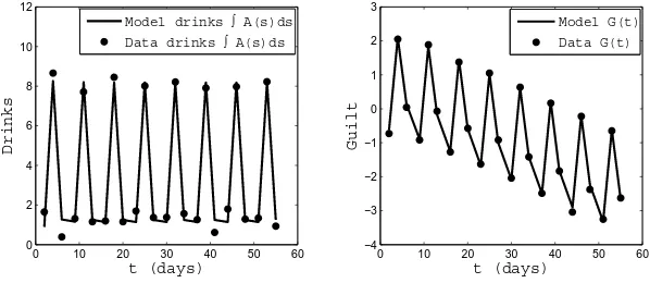
Interestingly, it appeared that one patient’s drinking pattern could be reasonably de-scribed when considering just two variables: the alcohol consumption rate A(t), and the guiltG(t). A key observation was that the individual’s drinking was driven by an innate re-ward/desire mechanism. This mechanism is the ingrained desire for drinking that separates problem drinkers from those who drink casually (or less). It is known that animals and human beings in particular yearn for something representing a reward, with the specific reward varying among individuals. Examples include food for some people, smoking for others, etc. In addition, it is known that individuals learn to turn this desire off when the reward is unavailable or they have decided they cannot indulge. So in addition to being a mechanism for desire it can also have the effect of controlling or limiting one’s intake of alcohol.

The model resulting from analysis of the data for this patient in such a context is given by

d

dtA(t) = −a12χ{G>G∗}(G(t)−G

∗_{) +a} 13h(t)

d

dtG(t) = a21

₀

−r

A(t+s)ds−(1 +cχ_{W(t)})A∗

(29)

where the functionh(t) represents the subject’s desire/reward mechanism, which increases going into the weekend (to turn it ‘on’), and decreases coming out of the weekend (thereby turning it ‘off’). This particular individual allowed himself to drink on the weekend as long as he refrains during the week, soh(t) has the form

h(ˆt) =

⎧ ⎪ ⎪ ⎪ ⎪ ⎨ ⎪ ⎪ ⎪ ⎪ ⎩

2(ˆt−1.5) 1.5≤ˆt <2 (Friday a.m. through Friday p.m.) −2(ˆt−2.5) 2≤ˆt <2.5 (Friday p.m. through Saturday a.m.) −2(ˆt−3.5) 3.5≤ˆt <4 (Sunday a.m. through Sunday p.m.)