University of South Carolina
Scholar Commons
Theses and Dissertations
2017
Nonparametric Inference for Orderings and
Associations Between two Random Variables
Chuan-Fa Tang
University of South CarolinaFollow this and additional works at:https://scholarcommons.sc.edu/etd
Part of theStatistics and Probability Commons
This Open Access Dissertation is brought to you by Scholar Commons. It has been accepted for inclusion in Theses and Dissertations by an authorized administrator of Scholar Commons. For more information, please [email protected].
Recommended Citation
Nonparametric inference for orderings and associations between two random variables
by Chuan-Fa Tang
Bachelor of Science
National Taiwan University 2007
Master of Science
National Taiwan University 2010
Submitted in Partial Fulfillment of the Requirements for the Degree of Doctor of Philosophy in
Statistics
College of Arts and Sciences University of South Carolina
2017 Accepted by:
Joshua M. Tebbs, Major Professor Dewei Wang, Major Professor John Grego, Committee Member Alexander McLain, Committee Member
c
•Copyright by Chuan-Fa Tang, 2017
Dedication
Acknowledgments
Thanks to my respectable mentors Dr. Joshua Tebbs and Dr. Dewei Wang
for their tireless forging
Thanks to my committee members Dr. John Grego and Dr. Alexander McLain
for their helpful suggestions
Thanks to my dear mother and brother Wang, Chin-Hao and Tang, Ming-Siang
for their kind support
Thanks to my dear father Tang, Su-Hsiang for his selfless dedication
Abstract
Table of Contents
Dedication . . . iii
Acknowledgments . . . iv
Abstract . . . v
List of Tables . . . ix
List of Figures . . . xi
Chapter 1 Introduction . . . 1
1.1 Literature review . . . 1
1.2 Outline . . . 4
Chapter 2 Nonparametric goodness-of-fit tests for uniform stochastic ordering . . . 5
2.1 Introduction . . . 5
2.2 Testing procedure . . . 11
2.3 Theoretical results . . . 12
2.4 Simulation evidence . . . 19
2.5 Premature infant data . . . 25
2.6 Concluding remarks . . . 27
Chapter 3 Empirical-likelihood-based testing for positive
quad-rant dependence . . . 37
3.1 Introduction . . . 37
3.2 Testing H0 versus H1≠H0 . . . 41
3.3 Testing H1 versus H2≠H1 . . . 44
3.4 Simulation results . . . 47
3.5 Real Data Analysis . . . 54
3.6 Conclusion . . . 59
Chapter 4 Extensions . . . 60
4.1 Nonparametric goodness-of-fit tests for uniform stochastic ordering (USO) with random right-censored data . . . 60
4.2 Empirical-likelihood-based testing for exchangeability . . . 65
Bibliography . . . 72
Appendix A Supplementary materials for Chapter 2 . . . 77
A.1 Lemmas . . . 77
A.2 Densities and critical values . . . 99
A.3 Supplementary material for Section 2.3.2 . . . 100
A.4 Supplementary material for Section 2.4 . . . 103
Appendix B Supplementary materials for Chapter 3 . . . 109
B.1 Proofs . . . 109
B.2 Supremum of empirical likelihoods under independence restriction . . 110
B.4 Critical values . . . 117
Appendix C Supplementary materials for Chapter 4 . . . 120
List of Tables
Table 3.1 Estimated probability of rejecting H0 with different sample size configurations and – = 0.05 for testing procedures EL1, EL2, EM, KS1, CvM1, and AD1 when samples of sizen are generated from a bivariate normal distribution with the marginal being standard normal and correlation coefficient being fl, where n is considered to be in{10,30,50,100}andfltakes values of 0, 0.25,
and 0.50. Note that, whenfl= 0, H0 is true; whenfl= 0.25 and
0.50, H1≠H0 is true. . . 49 Table 3.2 Estimated probability of rejecting H1 with different sample size
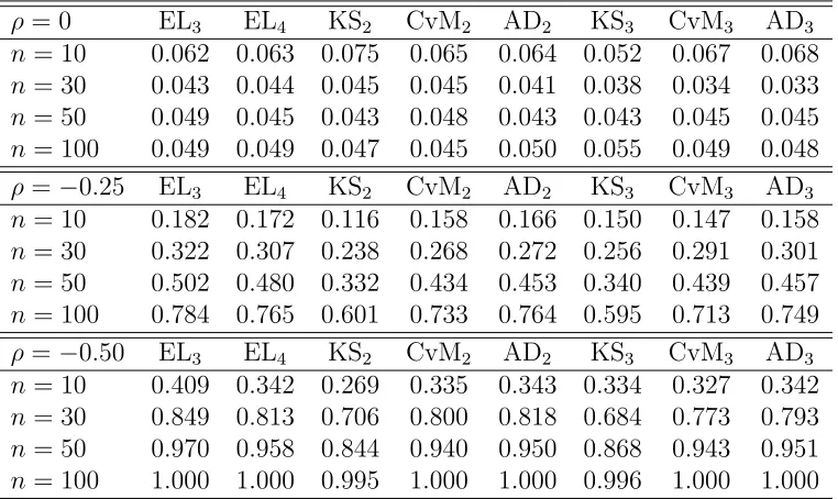
configurations and – = 0.05 for testing procedures EL3, EL4, KS2, CvM2, AD2, KS3, CvM3, and AD3 when samples of size n are generated from a bivariate normal distribution with the marginal being standard normal and correlation coefficient being
fl, where n is considered to be in {10,30,50,100} and fl takes
values of 0, ≠0.25, and ≠0.50. Note that, when fl = 0, H1 is
true; whenfl=≠0.25 and≠0.50, H2≠H1 is true. . . 52 Table 3.3 The dependence coefficients, Pearson’s rho, Kendall’s tau, and
Spearman’s rho are provided for three stock prices among APPL,
GOOGL, and WMT. . . 57
Table 4.1 Hamilton depression scale factor IV values on the tranquilizer,
provided in Hollander (1971). . . 71
Table A.1 Values of c–,p, the upper – quantiles of ÎD[0(1,,1]0)BÎp, for p œ
{1,2,3,5,Œ} and –= 0.01, 0.05, and 0.10. . . 100
Table A.2 Estimated probability of rejectingH0 :F ÆUSGforpœ{1,2,Œ}, different sample size configurations, and –= 0.05. All estimates
are based on 10,000 Monte Carlo data sets. ODCs R1, R2, R3,
and R4 satisfy H0. ODCsR5, R6, R7, and R8 satisfy H1. . . 105
Table A.3 Estimated probability of rejecting H0 :F ÆUS G, G known, for p œ {1,2,Œ} and – = 0.05. The GOF test from Arcones and
Table A.4 Minimum sample sizes to detect specific departures fromH0
us-ing –= 0.05 and power 1≠— = 0.8 for Ri œ 1. . . 108
Table B.1 Estimated critical values for test statistics generated by the inde-pendence copula with significance level– = 0.1,0.05,0.025,0.01.
10,000 Monte Carlo samples of size n = 10,30,50,100,200 are
used to estimate the critical values. . . 118
Table B.2 Estimated critical values for test statistics generated by the inde-pendence copula with significance level– = 0.1,0.05,0.025,0.01.
10,000 Monte Carlo samples of size n = 10,30,50,100,200 are
List of Figures
Figure 2.1 Ordinal dominance curves. Left: F ÆS G. Middle: F ÆUS G.
Right: F ÆLR G. In each subfigure, the equal distribution line
is shown dotted. . . 7
Figure 2.2 Premature infant data. Left: The sample ODC Rmn(u) =
Fm{G≠n1(u)}for the time to discharge (F = caffeine;G= no
caf-feine). Right: The least star-shaped majorantMRmn is shown
in blue. In each subfigure, the equal distribution line is shown
dotted. . . 8
Figure 2.3 Left: Star-shaped ODCs; i.e.,Ri œ 0. Right: Non-star-shaped
ODCs; i.e., Ri œ 1. A description of each curve is given in
Appendix A. . . 20
Figure 2.4 Local power family of ODCs indexed by” œ[0,0.5]. The”= 0
member R(0) is the initial ODC in 1; the ” = 0.5 member R(0.5) is the limiting ODC in 0. This family is described in
Appendix A. . . 24
Figure 2.5 Local power results with – = 0.05. Left: ’r = logr. Middle:
’r = r2/5. Right: ’r = r1/2. Top: Two-sample case. Bottom:
One-sample case. Our Lp results are shown dotted for p =
1, dashed for p = 2, and dot-dashed for p = Œ. Arcones
and Samaniego (2000) results (one-sample case only) are shown
using a solid line. . . 26
Figure 3.1 Rejection rates of testing procedures EL3, EL4, KS2, CvM2, AD2, KS3, CvM3, and AD3for the bivariate normal distribution with correlation flœ{≠0.5,≠0.4, . . . ,0.2} and sample size n = 100. The significance level is 0.05 which is depicted by a dotted
horizontal line. . . 53
Figure 3.2 Left: Rejection rates of testing procedures EL3, EL4, KS2, CvM2, AD2, KS3, CvM3, and AD3for Clayton copula (left) and Frank copula (right) with Kendall’s · œ {≠0.4,≠0.4, . . . ,0.1}
and sample sizen = 100. The significance level is 0.05 which is
Figure 3.3 Scatter plots of stock prices (the first row) and the correspond-ing pseudo-observations (the second row). From left to right are APPL versus GOOGL, APPL versus WMT, and GOOGL
versus WMT. . . 56
Figure A.1 Probability density function of ÎD(1[0,,1]0)BÎp for pœ{1,2,3,5,Œ}. . 99
Chapter 1
Introduction
1.1 Literature review
For a bivariate random vector (X, Y), one is usually interested in questions of how
X and Y are related. In this dissertation, we address two questions. If X and Y
are independent, which one is larger? If they are not independent, how might we adequately describe the dependence structure?
One way to compare the marginal distributions of X and Y is to compare their means. A two sample t-test can be used to order the means under normal assump-tions. However, without the normal distribution assumption, ordering the means may not be sufficient to describe the ordering between the distributions. To compare distributions more generally, we introduce three commonly used stochastic orderings in this dissertation.
andY being between two fixed numbers, one random variable tends to provide larger values. This type of ordering is useful theoretically and has important applications in finance and econometrics. It can be shown easily that likelihood ratio ordering is the strongest ordering among these three and that ordinary stochastic ordering is the weakest.
From the last paragraph, we can see that ease of interpretation is one of the ad-vantages of thinking in terms of stochastic orderings. More than that, order-restricted estimators are well-developed for each, and most of these estimators are better than their unrestricted versions when the corresponding ordering holds. For example, under ordinary stochastic ordering, El Barmi and McKeague (2005) developed re-stricted estimators for distribution functions and Davidov and Herman (2012) devel-oped restricted estimators for the area under the ordinal dominance curve (Bamber, 1975). They also showed that their estimators have smaller mean squared errors than those that are unrestricted. For uniform stochastic ordering restriction, Rojo and Samaniego (1993), Mukerjee (1996), Rojo (2004), and El Barmi and Mukerjee (2016) proposed restricted estimators of distribution functions. Rojo (2004) and El Barmi and McKeague (2005) showed that their proposed estimators have smaller mean squared errors.
Before using a restricted estimator, it is crucial to know if the corresponding stochastic ordering holds; otherwise, this may introduce unnecessary bias. In this dissertation, we focus on uniform stochastic ordering as described in Chapter 2. To reveal the existence of this ordering, we consider goodness-of-fit hypothesis problems; i.e., testing the uniform stochastic ordering assumption versus not. Previously pro-posed testing procedures (e.g., Park et al., 1998; Arcones and Samaniego, 2000) lose power due to discretizing the supports or overestimating critical values. To gain more power, we propose a new way to tackle this hypothesis testing problem.
majorant-based testing approaches described in Carolan and Tebbs (2005), Davidov and Herman (2012) and Beare and Moon (2015). In Chapter 2, we find that majorant-based methods for uniform stochastic ordering inherit good properties. Test statistics are easy to compute, and most importantly, the least favorable configurations exist (which helps to determine critical values and control Type I error probability). We provide an extension to incorporate random right-censored data in Chapter 4.
In this dissertation, we also focus on the positive quadrant dependence structure proposed by Lehmann (1966). A bivariate random vector (X, Y) is positive quadrant dependent (PQD) if the probability of X and Y of being simultaneously small is at least as large as it would be when X and Y are independent. The PQD property has useful applications in finance, insurance, and risk management. For example, if the true dependence structure of (X, Y) is PQD, then insurance premiums involving the portfolio containing X and Y will be underestimated if X and Y are treated as independent. See Dhaene and Goovaerts (1996), Denuit et al. (2001), Denuit and Scaille (2004), Embrechts et al. (2002) for more discussion. For applications in reliability theory and other ares, see Levy (1992), Shaked and Shanthikumar (1994), Drouet and Kotz (2001), and Lai (2003).
problematic if kernel estimation is involved, as it depends on bandwidth selection and is therefore potentially time-consuming and subjective.
To avoid these problems, we develop new hypothesis tests using empirical likeli-hood (Owen, 1990) to determine the existence of PQD between X and Y. Based on the empirical likelihood approach, many testing problems have been studied and have been shown to be powerful (Einmahl and McKeague, 2003; El Barmi and McKeague, 2013). We also expect these testing procedures to be powerful when testing for and against PQD.
1.2 Outline
In Chapter 2, we propose nonparametric goodness-of-fit tests for uniformly stochas-tic ordering with two continuous distributions based on the Lp difference between
Chapter 2
Nonparametric goodness-of-fit tests for
uniform stochastic ordering
Summary: We propose Lp distance-based goodness-of-fit (GOF) tests for uniform
stochastic ordering with two continuous distributions F and G, both of which are unknown. Our tests are motivated by the fact that when F and G are uniformly stochastically ordered, the ordinal dominance curve R = F G≠1 is star-shaped. We derive asymptotic distributions and prove that our testing procedure has a unique least favorable configuration of F and G for pœ[1,Œ]. We use simulation to assess
finite-sample performance and demonstrate that a modified, one-sample version of our procedure (e.g., with Gknown) is more powerful than the one-sample GOF test suggested by Arcones and Samaniego (2000, Annals of Statistics). We also discuss sample size determination. We illustrate our methods using data from a pharmacol-ogy study evaluating the effects of administering caffeine to prematurely born infants.
2.1 Introduction
function of G. When F =G, the ODC follows the main diagonal of the unit square, the so-called equal distribution line.
We consider order-restricted comparisons of F and G. Define F = 1≠F and G = 1≠G. These are the survivor functions if X and Y are lifetime random vari-ables, although herein we do not require X and Y to be nonnegative. Denote the corresponding densities by f and g, respectively. If F Æ G, then X and Y are stochastically ordered; this is written asF ÆS Gand means informally thatX “tends to be smaller” than Y. Two stronger orders are the uniform stochastic order and the likelihood ratio order. When F /G is nonincreasing, X and Y satisfy a uniform stochastic order, written F ÆUS G. When f /g is nonincreasing, X and Y satisfy a likelihood ratio order, writtenF ÆLR G. It is easy to show these orderings follow the nested structure: F ÆLR G =∆ F ÆUS G=∆F ÆS G. A comprehensive account of these and other orderings is given in Shaked and Shanthikumar (2007).
Different stochastic orderings give rise to different functional forms of the ODC. The weakest ordering F ÆS G holds if and only if R is at least as large as the equal distribution line; i.e., R(u) Ø u, for 0 Æ u Æ 1. The strongest ordering F ÆLR G holds if and only if R is concave. The intermediate ordering F ÆUS G holds if and only if R is star-shaped (Lehmann and Rojo, 1992). One way to characterize a star-shaped ODC is that the slope of the secant line from the point (1,1) to (u, R(u)); i.e., r(u) = {1≠R(u)}/(1≠u), is nonincreasing inu. Figure 2.1 gives examples of ODCs
that correspond to stochastic, uniform stochastic, and likelihood ratio orderings. This figure demonstrates the utility of the ODC in characterizing how two distributions are ordered and how the structure F ÆLR G =∆ F ÆUS G =∆ F ÆS G manifests itself graphically in the ODC.
0.0 0.2 0.4 0.6 0.8 1.0
0.0
0.2
0.4
0.6
0.8
1.0
u
R
(u
)
ODC
0.0 0.2 0.4 0.6 0.8 1.0
0.0
0.2
0.4
0.6
0.8
1.0
u
Star-shaped ODC
0.0 0.2 0.4 0.6 0.8 1.0
0.0
0.2
0.4
0.6
0.8
1.0
u
Concave ODC
Figure 2.1: Ordinal dominance curves. Left: F ÆS G. Middle: F ÆUS G. Right:
F ÆLR G. In each subfigure, the equal distribution line is shown dotted.
and n = 277 were not. Each infant was then followed until he or she was discharged from the hospital. All infants were eventually discharged and were alive at the time of discharge; i.e., no discharge times were censored. One of the goals of the study was to understand how the distributions of discharge times F (caffeine) and G (no caffeine) compared for the two groups. In Figure 2.2 (left), we display the sample ODC for the data, which is defined as Rmn(u) =Fm{Gn≠1(u)}, for 0Æ uÆ1, where
Fm and Gn are the empirical distribution functions and G≠n1(u) = inf{t:Gn(t)Øu}
is the empirical quantile function. The sample ODC and its large-sample properties were described in Hsieh and Turnbull (1996).
0.0 0.2 0.4 0.6 0.8 1.0
0.0
0.2
0.4
0.6
0.8
1.0
u
Rm
n
(
u
)
Empirical ODC
0.0 0.2 0.4 0.6 0.8 1.0
0.0
0.2
0.4
0.6
0.8
1.0
u
Rm
n
(
u
)
,
M
Rm
n
(
u
)
Least star-shaped majorant
Empirical ODC
Figure 2.2: Premature infant data. Left: The sample ODCRmn(u) =Fm{G≠n1(u)}for the
time to discharge (F = caffeine; G= no caffeine). Right: The least star-shaped majorant
MRmn is shown in blue. In each subfigure, the equal distribution line is shown dotted.
order-restricted class of alternatives; if the assumed class is incorrect, the test may lead to misleading or vacuous conclusions. For example, applying tests of this type to the premature infant data, we obtain the following results:
• testingF =G versusF ÆS G: p-value<0.00002 (Davidov and Herman, 2012)
• testing F = G versus F ÆUS G: p-value < 0.00001 (Arcones and Samaniego, 2000)
• testingF =G versusF ÆLR G: p-value <0.00001 (Carolan and Tebbs, 2005). Each test clearly dictates that the infant data are not consistent with F =G. How-ever, we are no closer to identifying which specific ordering (if any) holds in this setting.
nonparametric GOF tests with two distributions is more sparse, perhaps because this type of testing problem is more difficult. The primary reason for the added difficulty is that the ordering can hold under different configurations ofF and G. Therefore, one must determine the least favorable configuration of the two distributions before the test can be performed; i.e., so that the probability of type I error can be controlled. Carolan and Tebbs (2005) proposed nonparametric GOF tests for likelihood ratio ordering with two continuous distributions by using the least concave majorant of the sample ODC. This work was generalized and improved upon by Beare and Moon (2015) in the econometrics literature, who considered likelihood ratio ordering and its applications in finance.
GOF tests for uniform stochastic ordering have been proposed but only in lim-ited settings. Dardanoni and Forcina (1998) considered likelihood-based tests against uniform stochastic ordering in a two-way contingency table. Park et al. (1998) used a nonparametric maximum likelihood approach to formulate GOF tests with two or more continuous distributions, but only after data from these distributions have been assigned to disjoint intervals in the form of counts. This essentially discretizes the problem and results in testing against uniform stochastic ordering among several multinomial distributions. Furthermore, this formulation gives rise to non-unique least favorable configurations that depend on how the intervals are selected, the number of distributions, and even the significance level used. Finally, in the two-population setting, Arcones and Samaniego (2000) suggested a GOF test for uniform stochastic ordering based on the family of order-restricted estimators in Mukerjee (1996). However, these authors assume that one of the population distributions is known (e.g., G is known) and do not determine the least favorable configuration for their procedure. Instead, the authors use critical values from an upper bound asymptotic distribution which leads to a conservative test.
order-ing with two continuous distributions F and G; that is, we are interested in testing
H0 : F ÆUS G versus H1 : F ⇥US G, where both distributions are unknown. Mo-tivated by the ODC approaches taken in Carolan and Tebbs (2005) and Beare and Moon (2015), we construct test statistics forH0 versus H1 based on the Lp difference between the sample ODC and its least star-shaped majorant (defined in Section 2.2). We then derive asymptotic distributions and prove that our testing procedure has a unique least favorable configuration for p œ [1,Œ]. Interestingly, this theoretical
result is different from the finding in Beare and Moon (2015), who showed that when using Lp distance-based GOF tests for likelihood ratio ordering, the least favorable
configuration exists only when pœ[1,2]. Furthermore, unlike Park et al. (1998), our approach does not require one to discretize the support of the distributions which can only lead to a loss in power. Finally, we show that the one-sample version of our test (e.g., withG known) is not as conservative as the test proposed by Arcones and Samaniego (2000) and is generally better equipped to detect departures from H0.
Formulating Lp distance-based GOF tests for uniform stochastic ordering in the
adminis-tering caffeine is consistent with shorter discharge times. Note that, in this context, stochastic ordering requires that the relationship above hold only initially (i.e., when
t0 = 0). Uniform stochastic ordering guarantees this type of dominance will hold for
allt0 Ø0.
2.2 Testing procedure
Suppose that X1, X2, ..., Xm are independent and identically distributed (iid) fromF
and that Y1, Y2, ..., Yn are iid from G. We assume the two samples are independent
and that bothF andGare unknown. LetR=F G≠1denote the corresponding ODC. For our asymptotic results in Section 2.3 to hold, as in Hsieh and Turnbull (1996), we assumeF andG have continuous densities f and g and that the first derivative ofR is bounded over [0,1]. Throughout this chapter, we denote the parameter space ofR by , the collection of nondecreasing, continuously differentiable functions from [0,1] to [0,1]. Under our assumptions, the hypotheses H0 : F ÆUS G and H1 : F ⇥US G can be expressed equivalently as
H0 :Rœ 0 ={◊œ :◊ is star-shaped} and H1 :R œ 1 = \ 0.
Recall that ◊œ is star-shaped if and only if {1≠◊(u)}/(1≠u) is nonincreasing in
u.
Let Rmn = Rmn(u) = Fm{G≠n1(u)} denote the sample ODC, defined in Section
2.1. Informally, our testing procedure is based on measuring the distance between
Rmn and an estimate of R subject to the constraint that F ÆUS G. Towards defining
this restricted estimator, let l([0,1]) denote the collection of bounded functions on [0,1]. For anyh œl([0,1]), its least star-shaped majorant is defined as
Mh= inf{hú œl([0,1]) :hÆhú and hú is star-shaped};
majorant operator. Just asRmn is an estimator ofR under no restriction (Hsieh and
Turnbull, 1996), the least star-shaped majorant MRmn is an estimator of R under
H0 : F ÆUS G. Using Lemma A.1 in Appendix A, we show that this restricted estimator can be calculated as
MRmn(u) = 1≠ min vœVfi{0}
vÆu I
1≠Rmn(v)
1≠v
J
(1≠u),
for 0 Æ u < 1, where V is the set of discontinuous (jump) points of Rmn and MRmn(1) = 1. Figure 2.2 (right) shows the least star-shaped majorant of the sample
ODC for the premature infant data described in Section 2.1.
Our testing procedure utilizes the sample ODC Rmn and its least star-shaped
majorant MRmn. Specifically, we propose the family of test statistics
Mmnp =cmnÎMRmn≠RmnÎp,
wherecmn ={mn/(m+n)}1/2 is a normalizing constant andηÎp is theLp norm with
respect to Lebesgue measure. We allow forpœ[1,Œ]; i.e., ÎhÎp = (s[0,1]|h(u)|pdu)1/p
whenp < ŒandÎhÎŒ = supuœ[0,1]|h(u)|. For example, whenp= 1,ÎMRmn≠RmnÎ1
equals the area between the two estimators; when p=Œ, ÎMRmn≠RmnÎŒ equals the largest vertical distance between the estimators. For any pœ[1,Œ], clearly large values of Mp
mn are evidence againstH0.
2.3 Theoretical results
In this section, we first describe the asymptotic distribution of Mp
mn for any
star-shaped ODC; i.e., for any R œ 0. We then demonstrate that, for any p œ [1,Œ], all null distributions are dominated stochastically by the asymptotic distribution of
Mp
mn under R(u) = u, that is, when F =G. From this least favorable distribution,
we can find the critical value c–,p that satisfies limm,næŒpr(Mmnp Ø c–,p) =– when
words, rejecting H0 when Mmnp Øc–,p is an asymptotic size – decision rule. Finally,
we examine relevant asymptotic distributions when R œ 1 and then characterize large-sample power properties. We also discuss sample size calculations to detect departures from H0. All theorems are proved in Section 2.7. Additional technical details are provided in Appendix A.
2.3.1 Asymptotic results under H0
Let I denote the identity operator on l([0,1]) and define D = M≠I. When H0 is true; i.e., when Rœ 0, note that MR =R and
Mmnp =cmnÎMRmn≠RmnÎp =cmnÎDRmn≠DRÎp.
At first glance, establishing the limiting distribution ofMp
mn underH0 might seem to
be straightforward, that is, one could simply start with the asymptotic distribution of
cmn(Rmn≠R) described in Hsieh and Turnbull (1996) and apply the functional delta
method (see, e.g., Section 2.3.9 in Vaart and Wellner, 1996) and continuous mapping theorem. This was the approach taken by Beare and Moon (2015) with their Lp
distance-based GOF test statistics under likelihood ratio ordering. In our setting, this direct approach is not possible because whereas the least concave majorant op-erator in Beare and Moon (2015) is Hadamard directionally differentiable (Shapiro, 1990; Shapiro, 1991), the least star-shaped majorant operator M (and hence D) is
not always so; see Lemma A.5 in Appendix A. Fortunately, this does not create insurmountable problems because weak convergence of cmn(DRmn ≠DR) is not a
necessary prerequisite to derive the asymptotic distribution ofcmnÎDRmn≠DRÎp.
Before we state the asymptotic distribution of Mp
mn for any R œ 0, we need
to describe R precisely because these distributions depend completely on the shape of R. Recall that when R œ 0, the slope function r(u) = {1≠R(u)}/(1≠u) is nonincreasing in u. When r(u) is strictly decreasing over [0,1], we say that R is
to Beare and Moon (2015), there exists a unique collection (finite or countable) of closed, pairwise disjoint intervals of the form [ak, bk], 0 Æak < bkÆ1, where
• the sloper(u) is constant over each interval (i.e., R is affine over each interval)
• no two intervals possess the same value of r(u).
In this case, we say thatRœ 0 is non-strictly star-shaped. The reason we bifurcate 0 using “strictly” and “non-strictly” descriptors is that the nondegenerate part of
the asymptotic distribution of Mp
mn depends only on those regions where R is
non-strictly star-shaped. If R is strictly star-shaped over [0,1], the distribution of Mp mn
collapses to zero in the limit.
To make our description of the asymptotic distributions precise, we therefore introduce the following notation. For 0Æa < bÆ1, define
M(1[a,b,0)]h= inf{hú œl([0,1]) : hÆhú and hú is star-shaped
over [a, b] with kernel (1,0)}.
A general definition of what it means for a function hú to be star-shaped with kernel (c, d) is given directly before Lemma A.1 in Appendix A. For any h œ l([0,1]), the functionM(1[a,b,0)]hhas two defining characteristics. First, M
(1,0)
[a,b]h(u) = h(u) whenever
u /œ [a, b]. Second, over [a, b], M(1[a,b,0)]h is the smallest function (at least as large as
h) that is star-shaped with kernel (1,0); i.e., the slope function ≠M(1[a,b,0)]h(u)/(1≠u)
over [a, b] is nonincreasing in u. The importance of the functional operator M(1[a,b,0)] :
l([0,1])‘æl([0,1]) becomes clear as we state our first main result.
Theorem 2.1. Suppose R œ 0 and let B denote a standard Brownian bridge. The
asymptotic results below hold when min{m, n}æ Œ and n/(m+n)æ⁄œ(0,1).
(a) If R is strictly star-shaped over [0,1], then Mp mn
d
≠æ0 for all pœ[1,Œ]. (b) If R is non-strictly star-shaped, then for pœ[1,Œ),
Mmnp ≠æd
I ÿ
k Ë
⁄RÕ(ak) + (1≠⁄){RÕ(ak)}2
Èp/2⁄ bk
ak
Ó
D[(1ak,0),bk]B(u)
Ôp
du
J1/p
when p=Œ,
Mmnp ≠æd sup
k
IË
⁄RÕ(ak) + (1≠⁄){RÕ(ak)}2 È1/2
sup
uœ[ak,bk]
Ó
D[(1ak,0),bk]B(u)
ÔJ
.
In both asymptotic distributions, RÕ is the derivative of R and D(1,0)
[ak,bk]=M
(1,0)
[ak,bk]≠I.
From Theorem 2.1, one can see that when F ÆUS G, the only randomness in the asymptotic distribution of Mp
mn arises from the non-strictly star-shaped regions
[ak, bk] and is described probabilistically by the D(1[ak,0),bk]B processes. Furthermore,
when F = G, the asymptotic distribution of Mp
mn simplifies to ÎD
(1,0)
[0,1]BÎp for all
pœ [1,Œ]. When p= 1, for example, this quantity describes the distribution of the area between the least star-shaped majorant of a standard Brownian bridgeB and B
itself. When p=Œ, ÎD[0(1,,1]0)BÎŒ describes the distribution of the sup-norm distance between these two processes. Readers familiar with the GOF tests for likelihood ratio ordering in Carolan and Tebbs (2005) and Beare and Moon (2015) will no doubt recognize the homology between our Theorem 2.1 and the corresponding results in these articles. However, as noted earlier, GOF tests for uniform stochastic ordering present their own set of mathematical challenges and different conclusions are reached about the existence of a least favorable configuration.
Theorem 2.2. Suppose R œ 0. For any p œ [1,Œ], the asymptotic distribution of
Mp
mn is ordinary stochastically smaller than ÎD
(1,0)
[0,1]BÎp; i.e.,
lim
m,næŒ
n/(m+n)æ⁄
prRœ 0(Mp
mnØt)Æpr(ÎD
(1,0)
[0,1]BÎp Øt), for all t œR, where ⁄ is defined in Theorem 1.
Theorem 2.2 establishes that when using Mp
mn to test H0 : F ÆUS G versus
H1 : F ⇥US G, the equal distribution line R(u) = u represents the least favorable
startling discovery because each process shares the same Brownian bridge B and
each operator D[(1ak,0),bk] shares the same kernel point (1,0). The practical utility of
Theorem 2.2 is that, for any p œ [1,Œ], we can determine the critical value that maximizes the probability of type I error over all configurations of F and G in 0. This result is different than the conclusion reached in Beare and Moon (2015), who showed that when testing against likelihood ratio ordering using Lp distance-based
statistics involving the least concave majorant ofRmn,R(u) = uis the least favorable
configuration when pœ[1,2] and for p >2 the least favorable configuration does not exist. Careful inspection of Theorem 2.1 and some intuition sheds insight on why this is true. When R is star-shaped, but not strictly star-shaped, each of the derivatives
RÕ(a
k) in Theorem 2.1 satisfies RÕ(ak) Æ 1. However, when F ÆLR G, there is
no guarantee these derivatives are uniformly bounded for all concave R and hence anomalous limiting behavior can result when pis too large.
For given values of the significance level–andpœ[1,Œ], denote the 1≠–quantile
of ÎD[0(1,,1]0)BÎp by c–,p; i.e., c–,p solves – = pr(ÎD[0(1,,1]0)BÎp Øc–,p). To approximate the
distribution of ÎD(1[0,,1]0)BÎp, we generated 100,000 Brownian bridge paths on a grid of
100,000 equally spaced points in [0,1], and, for eachpœ{1,2,3,5,Œ}, we calculated
ÎD(1[0,,1]0)BÎp for each path. For each p, these 100,000 values were used to approximate
the density function of ÎD(1[0,,1]0)BÎp and quantiles c–,p, for – = 0.01, 0.05, and 0.10.
These functions and the selected quantilesc–,p are provided in Appendix A.
2.3.2 Asymptotic results under H1
The difference between the asymptotic distribution of Mp
mn under H0 : R œ 0 and
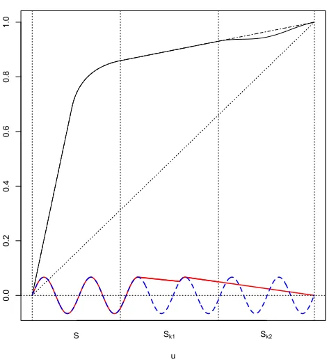
that underH1 :R œ 1 arises from the non-star-shaped regions ofR. To characterize a non-star-shaped ODCR œ 1, start withMR, which is star-shaped, and note that (as in Section 2.3.1) one can partition the unit interval [0,1] as [0,1] = Sfi(fikSk),
disjoint intervals of the form Sk = [ak, bk], 0Æak < bk Æ1, for k = 1,2, .... One can
further partition each Sk as Sk =Sk1fiSk2, where Sk1 ={u œSk :MR(u) =R(u)}
andSk2 ={uœSk :MR(u)> R(u)}. Each Sk1 must containakso it is never empty,
and the non-star-shaped regions ofRcan be written asfikSk2. In other words,Rœ 0
when fikSk2 is empty and Rœ 1 otherwise.
In general, these types of regions contribute differently to the limiting distribution of Mp
mn. Over the strictly star-shaped region S, MR(u) = R(u) for all u and the Lp
norm of cmn{DRmn(u)≠DR(u)} converges in distribution to 0, as in Section 2.3.1.
To clearly describe the contribution over theSk regions, we introduce new notation.
For anyhœl([0,1]), define the functional operatorLSk :l([0,1])‘æl([0,1]) according
to
LSkh(u) = ≠ inf
vœSk1 vÆu
I
≠h(v)
1≠v
J
(1≠u)ISk(u) +h(u)ISkc(u), for uœ[0,1),
whereIA(·) is the indicator function over the setAandAc denotes the complement of
A. Whenu= 1,LSkh(u) = max{h(1),0}orh(1) depending on whether the singleton
{1} œ Sk1 or not; see Appendix A. Using this new operator, we now characterize
asymptotic distributions for any ODCR œ with those in 1 = \ 0 of particular interest. A discussion on the large-sample power properties of our testing procedure follows.
Theorem 2.3. Suppose R œ . Using the notation described in this subsection,
cmnÎDRmn≠DRÎp ≠æd I
ÿ
k ⁄
uœSk
--LSkT
⁄
R(u)≠TR⁄(u)
--pdu
J1/p
for pœ[1,Œ); when p=Œ,
cmnÎDRmn≠DRÎp ≠æd sup k usupœSk
--LSkT
⁄
R(u)≠TR⁄(u)
--.
Both results hold as min{m, n} æ Œ and n/(m+n) æ ⁄ œ (0,1). In both cases,
T⁄
Four remarks are in order. First, the process T⁄
R = {TR⁄(u),0 Æ u Æ 1} in
Theorem 2.3 is well known; as noted earlier, it represents the asymptotic distribution ofcmn(Rmn≠R) for anyR œ ; see, e.g., Theorem 2.2 in Hsieh and Turnbull (1996).
Second, the asymptotic distributions identified in Theorem 2.3 apply for any R œ , but we show in Appendix A that they quickly reduce to those in Theorem 2.1 when
R œ 0. Third, our Lp tests are consistent for p œ[1,Œ]. To see why, consider the sup-norm (p=Œ) case in Theorem 2.3 and note that, by the triangle inequality,
prRœ 1(MmnŒ Øc–,Œ) = prRœ 1 1
cmnÎDRmnÎŒØc–,Œ
2
Ø prRœ 1 1
cmnÎDRmn≠DRÎŒÆcmnÎDRÎŒ≠c–,Œ
2
which can be approximated by
prRœ 1 3
sup
k usupœSk
--LSkT
⁄
R(u)≠TR⁄(u)
--ÆcmnÎDRÎŒ≠c–,Œ
4
.
It is easy to show that supksupuœSk|LSkT
⁄
R(u)≠TR⁄(u)| is bounded and that, for any
R œ 1, cmnÎDRÎŒ æ Œ, as min{m, n} æ Œ, which establishes our claim. The finitep argument is analogous. Fourth, approximate lower bounds on the power, like the one above in the sup-norm case, can be used for sample size calculations. For an ODCR œ 1 deemed to be clinically relevant, one can determine numerically the smallestm andn that solve prRœ 1(supksupuœSk|LSkT
⁄
R(u)≠TR⁄(u)|ÆcmnÎDRÎŒ≠
c–,Œ) = 1≠—, where— œ(0,1). The resulting solution will be inexorably conservative but still potentially useful for planning purposes. We illustrate this approach with examples in Section 2.4.
a sequence of ODCs in 1. For each r Ø 1, denote the corresponding distributions byF(r) and G(r) from which we have independent random samples X(r)
1 , X2(r), ..., Xm(r)
and Y1(r), Y2(r), ..., Y(r)
n , respectively. We examine local power properties by letting
R(r) approach
0 in the sense that ÎDR(r)Îp = ÎMR(r)≠R(r)Îp æ 0 as r æ Œ at
different rates. Using the notation in this paragraph, our last theorem summarizes the salient results.
Theorem 2.4. Suppose the first derivative of R(r) œ
1 is uniformly bounded over
[0,1]for all r. Suppose pœ[1,Œ]. All limits stated below assume that max{m, n}= O(r) and n/(m+n)æ⁄ œ(0,1), as ræ Œ.
(a) If limcmnÎDR(r)Îp =Œ, then lim prR(r)œ 1(Mmnp > c–,p) = 1.
(b) For any — œ(0,1), there exists ÷p(—)>0 such that
lim inf prR(r)œ 1(Mmnp > c–,p)Ø1≠—
whenever lim infcmnÎDR(r)Îp Ø÷p(—).
Part (a) of Theorem 2.4 indicates that when ÎDR(r)Î
p converges to 0 at a rate
slower thanc≠1
mn,cmnÎDR(r)Îp diverges and the power of our test converges to 1. Part
(b) guarantees that when cmnÎDR(r)Îp remains bounded away from zero, the power
of our test is still nontrivial; i.e., it does not converge to 0. This occurs when the “amount of information”cmn increases and the “departure” ÎDR(r)Îp decreases, and
both do so at the same rate.
2.4 Simulation evidence
0.0 0.2 0.4 0.6 0.8 1.0
0.0
0.2
0.4
0.6
0.8
1.0
u
R
(u
)
R1
R2
R3
R4
0.0 0.2 0.4 0.6 0.8 1.0
0.0
0.2
0.4
0.6
0.8
1.0
u
R
(u
)
R5
R6 R7
R8
Figure 2.3: Left: Star-shaped ODCs; i.e., Ri œ 0. Right: Non-star-shaped ODCs; i.e.,
Ri œ 1. A description of each curve is given in Appendix A.
procedure to allow for one of the population distributions to be known and compare this modified test to the one-sample GOF test in Arcones and Samaniego (2000). Local power results are provided in Section 2.4.3.
2.4.1 Fixed ODC comparisons
We consider four ODCs satisfying R œ 0 (R1, R2, R3, and R4) and four ODCs satisfying R œ 1 (R5, R6, R7, and R8). The H0 ODCs (Figure 2.3, left) are each members of a family of star-shaped ODCs that we describe in the Appendix A. The
H1 ODCs (Figure 2.3, right) are not star-shaped and are also described in Appendix
A. We also consider R0 = R0(u) = u, for u œ [0,1], to examine finite-sample performance under the least favorable configuration F = G. All of our results are based on 10,000 Monte Carlo data sets using independent samples fromF andGwith sample sizes m and n, respectively. To generate the samples, we let F(u) = Ri(u)
andG(u) =u, for uœ[0,1]. We then sampleX1, X2, ..., Xm fromF using the inverse
from a uniform(0,1) distribution. This provides independent samples for each ODC
R under consideration.
Table A.2 in Appendix A gives Monte Carlo estimates of the probability of reject-ing H0 : F ÆUS G for different sample sizes, values of p œ {1,2,Œ}, and – = 0.05. We experimented with other values of p (i.e., p= 3 and p= 5) but obtained results similar to those whenp= 2. Of initial interest is the finite-sample performance when
F = G. With 10,000 simulated data sets, the margin of error associated with the
size estimates underF =G, assuming a 99 percent confidence level, is approximately 0.006. Therefore, one notes that our tests with p = 1 and p = 2 are slightly anti-conservative with small samples and otherwise operate closely to the nominal level. Furthermore, examining the rejection rates for the other star-shaped ODCs (R1, R2,
R3, and R4) supports Theorem 2.2 which, for p œ[1,Œ], guarantees the probability of type I error will be at its maximum under F =G. Likewise, powers for the non-star-shaped ODCs (R5, R6,R7, andR8) all approach unity as mandn become large. This reinforces our consistency claim.
We also use the non-star-shaped ODCs in Figure 2.3 to illustrate sample size determination. For p œ [1,Œ] and for a given R œ 1, denote by dR,—,p the 1≠—
quantile of the asymptotic distributions in Theorem 2.3. Using our lower bound on the asymptotic power from Section 2.3.2 and taking m = n (for simplicity), we obtain a closed-form expression for the minimum sample size necessary to detect the departure ÎDRÎp = ÎMR≠RÎp with probability 1≠— when using an asymptotic
size – test; i.e.,
m= 2
A
dR,—,p+c–,p
ÎDRÎp
B2
, for pœ[1,Œ].
With – = 0.05 and 1≠— = 0.8, Appendix A tables these solutions for each
non-star-shaped ODC in Figure 2.3 and for each p œ {1,2,Œ}. For example, for the
R5 ODC, which corresponds to F and G being stochastically ordered (but not
respectively, are m = 634, m = 461, and m = 582. Such sample sizes might seem dispiritingly large; however, it is not surprising these solutions are conservative. We describe in Section 2.6 alternative approaches that should reduce this conservatism.
2.4.2 Comparison with Arcones and Samaniego (2000)
We now turn our attention to the special case of testing H0 : F ÆUS G versus H1 : F ⇥US G where G is known. Arcones and Samaniego (2000), who focused
largely on optimal estimation of F (with F ÆUS G and G known), also suggested a conservative large-sample procedure to test againstH0. Their proposed test statistic, which we denote by Dm, can be expressed as a function of the one-sample ODC
Rm =FmG≠1; specifically,
Dm =m1/2 sup
0ÆvÆuÆ1[(1≠v){1≠Rm(u)}≠(1≠u){1≠Rm(v)}].
However, instead of deriving a least favorable (asymptotic) distribution for inference, the authors proved that the asymptotic distribution of Dm is bounded above by
2 supuœ[0,1]|B(u)|, where B is a standard Brownian bridge, and selected their critical
value cAS–/2 to satisfy –= pr(supuœ[0,1]|B(u)| ØcAS–/2). On the other hand, one-sample versions of our GOF procedure are available and use the test statistics
Mmp =m1/2
C ⁄
[0,1]{DRm(u)}
pdu
D1/p
and MmΠ=m1/2 sup
uœ[0,1]{D
Rm(u)},
where D is the operator defined in Section 2.3.1 and Rm(u) = Fm{G≠1(u)}. The
limiting distributions in Theorem 2.1 also apply here as m æ Œ; in addition, it is
straightforward to modify the proof of Theorem 2.2 to conclude that F =G admits the least favorable configuration forpœ[1,Œ] in the known G case.
For different sample sizesm(now corresponding toF only), Table A.3 in Appendix A gives small-sample rejection rates of our one-sample tests and the test from Arcones and Samaniego (2000), both performed using–= 0.05. We used techniques similar to
and performed all simulations in the same way as before except G is now known. Clearly, there is a price to be paid for using the test based on theDm statistic when
F =G; type I error probability estimates remain significantly below the nominal level
for all m Æ 200. On the other hand, our p = 1 and p = 2 tests are only minimally conservative whenm Æ75, and our sup-norm (p=Œ) test performs nominally even
when m = 20. In addition, the sup-norm test can be markedly more powerful at detecting non-star-shaped alternatives with small to moderately sized samples.
2.4.3 Local power analysis
A consequence of Theorem 2.3 is that, for any fixed R œ 1, our Lp GOF tests are consistent for all p œ[1,Œ]. To glean additional insight on which values of p might be preferred in practice, we investigate the power associated with local alternatives. Starting in the lower left corner, Figure 2.4 depicts a sequence of ODCs in 1 that approach 0 (moving from lower left to upper right). Each ODC shown in Figure 2.4 belongs to a family of ODCs described in Appendix A; the defining feature of this family is that it is indexed by a single parameter ” œ [0,0.5]. The ” = 0
member, say R(0), is the initial ODC in the lower left corner of Figure 2.4; the
” = 0.5 member R(0.5), shown in the upper right, is the limiting ODC in 0. ODCs
R(”) with intermediate values of ”œ(0,0.5) are also identified in Figure 2.4.
In our testing problem, a local power analysis involves examining a sequence of ODCs {R(r), r = 1,2, ...,} in
1 that converges to 0 at different rates. We do so
here by using the family of ODCs just described. Specifically, we consider the rates
’r œ {logr, r2/5, r1/2}. For each ’r, we first choose a sequence of constants ”(r) such
that limr挒r|”(r)≠0.5| = c’r > 0 and then select members from our ODC family
identified by R(r) = R
(”(r)), for r = 1,2, .... The resulting sequence R(r) satisfies
ÎDR(r)Î
p = ÎMR(r) ≠R(r)Îp æ 0 and ’rÎDR(r)Îp æ cú’r,p > 0, both as r æ Œ.
0.0 0.2 0.4 0.6 0.8 1.0
0.0
0.2
0.4
0.6
0.8
1.0
u
R
(u
)
δ=0
δ=0 .1
δ=0 .2
δ=0 .3
δ=0
.4
δ=0 .5
Figure 2.4: Local power family of ODCs indexed by” œ[0,0.5]. The ”= 0 member R(0)
is the initial ODC in 1; the”= 0.5 member R(0.5) is the limiting ODC in 0. This family
is described in Appendix A.
(i.e., with bothF and G unknown). We also use these ODC sequences, one for each rate ’r, to compare the one-sample versions of our tests with the test in Arcones and
Samaniego (2000).
For each r œ {50,100,500,1000,5000,10000}, we simulated 10,000 independent
random samples, X1(r), X2(r), ..., Xm(r) from F(r) and Y
(r)
1 , Y2(r), ..., Yn(r) from G(r),
where F(r)(u) = R(r)(u) and G(r)(u) = u, 0 Æ u Æ 1, and m = n = r. Figure 2.5
(top row) shows the estimated powers of our–= 0.05 tests associated with each rate:
’r= logr(left), ’r =r2/5 (middle), and’r =r1/2 (right). Note that with m=n=r,
considering the slower rates ’r = logr and ’r = r2/5 allows us to assess part (a) of
Theorem 2.4, while the fastest rate’r =r1/2 allows us to assess part (b). Both parts
powers hover only slightly above 0.3 for allr, while the p= 2 andp=Œpowers still approach unity.
Switching to the one-sample problem, we find quite different results. For each rate ’r, Figure 2.5 (bottom row) displays the estimated powers of our one-sample
–= 0.05 tests which use Mm1,Mm2, andMŒ
m. Powers were estimated in the same way
as for the two-sample case except now we treatG(r)(u) =uas known and takem=r.
In this setting, the sup-norm test consistently provides the largest power, followed by the p = 2 test and the p = 1 test. In addition, all three distance-based tests outperform the corresponding– = 0.05 Arcones and Samaniego (2000) test in terms
of local power, especially at the fastest rate ’r = r1/2 where prR(r)œ 1(Dm > cAS0.025)
appears to decrease towards zero.
2.5 Premature infant data
Caffeine is commonly used to treat newborn infants for apnea of prematurity (Schmidt et al., 2006) and to prevent the onset of respiratory distress syndrome, bronchopul-monary dysplasia, and extubation failure (Cox et al., 2015). Known as “the silver bullet” in the treatment of prematurely born infants at risk for these and other acute conditions (Aranda et al., 2010), caffeine is widely regarded within the neonatal care community to be safe and cost effective. It has also been approved by the United States Food and Drug Administration for use with preterm infants due to its history of providing beneficial outcomes with no long-term adverse side effects (Dobson and Hunt, 2013).
0.0
0.2
0.4
0.6
0.8
1.0
Po
w
e
r
log 50 log 500 log 5000
0.0
0.2
0.4
0.6
0.8
1.0
log 50 log 500 log 5000
0.0
0.2
0.4
0.6
0.8
1.0
log 50 log 500 log 5000
0.0
0.2
0.4
0.6
0.8
1.0
Log sample size
Po
w
e
r
log 50 log 500 log 5000
0.0
0.2
0.4
0.6
0.8
1.0
Log sample size
log 50 log 500 log 5000
0.0
0.2
0.4
0.6
0.8
1.0
Log sample size
log 50 log 500 log 5000
Figure 2.5: Local power results with – = 0.05. Left: ’r= logr. Middle: ’r=r2/5. Right: ’r=r1/2. Top: Two-sample case. Bottom:
One-sample case. Our Lp results are shown dotted for p = 1, dashed for p = 2, and dot-dashed for p =Œ. Arcones and Samaniego
(2000) results (one-sample case only) are shown using a solid line.
no-caffeine groups, respectively, recall that Figure 2.2 displays the sample ODC Rmn
and its least star-shaped majorant MRmn, calculated from samples of size m = 127
from F and n = 277 from G. As noted in Section 2.1, we performed the test in Davidov and Herman (2012) with these data and concluded thatF ÆSGwas strongly supported overF =G. We also performed the GOF tests in Beare and Moon (2015) and concluded thatF ÆLR Gwould be rejected at –= 0.05; the L1 and L2 statistics based on the least concave majorant of Rmn are 0.717 and 0.999, respectively, which
are larger than the corresponding 0.95 quantiles 0.664 and 0.753 identified by their least favorable distributions.
We therefore assess whether or not the data in Figure 2.2 are consistent with uniform stochastic ordering. Testing H0 : F ÆUS G versus H1 : F ⇥US G based on the least star-shaped majorant of Rmn, our GOF test statistics are Mmn1 = 0.170,
Mmn2 = 0.263, andMmnΠ= 0.949, each of which is well below theР= 0.10 critical
val-ues identified in Appendix A (0.496, 0.586, and 1.219, respectively), that is,H0cannot be discounted at any reasonable level of significance. Therefore, not only does caf-feine therapy provide point-of-care health benefits and improved long-term outcomes for prematurely born infants, our analysis suggests that treating these infants with caffeine may also lead to hospital discharge times that are uniformly stochastically smaller than those for infants not treated with caffeine.
2.6 Concluding remarks
related applications. In this situation, one could apply our tests after conditioning to determine if R is non-star-shaped over the smaller region [G≠1(t0),1] and calculate sample sizes to detect departures over it instead of over [0,1]. A similar approach was suggested by Carolan and Tebbs (2005) for detecting departures from likelihood ratio ordering. In the same spirit, Beare and Moon (2015) suggest that bootstrapping samples over departure regions could help to increase the power of GOF tests for likelihood ratio ordering. This strategy may also be fruitful in our setting, allowing one to reduce the conservatism arising from relying on the least favorable distribution over the entire unit interval.
We believe that our GOF tests could be generalized to allow for different types of censored data, but the theory underpinning these extensions would not be trivial. For example, with random right-censored data, there would be nothing to prevent one from simply replacing the empirical survival functions Fm and Gn with
Kaplan-Meier estimators of F and G and then calculating Rmn and MRmn using these
es-timates. However, asymptotic distributions of the corresponding test statistics may depend heavily on the latent censoring distributions, and there is no guarantee that the least favorable configuration of F and G will exist. Future work could inves-tigate censored-data extensions of majorant-based inference≠not only with uniform
stochastic ordering, but with other orderings as well.
Lemma A.4 in Appendix A. Another interesting avenue for future research would be to generalize our majorant-based tests to more than two populations. Estimation techniques in this setting are available in Dykstra et al. (1991) and El Barmi and Mukerjee (2016).
2.7 Proofs
In this section, we provide the proofs of Theorems 2.1-2.4. Lemmas cited in this section are stated and proved in Appendix A.
Proof of Theorem 2.1. We start with the asymptotic distribution of Rmn, suitably
centered and scaled. Applying Theorem 2.2 in Hsieh and Turnbull (1996), it follows that cmn(Rmn ≠R) converges weakly to TR⁄ as min{m, n} æ Œ and n/(m+n) æ
⁄ œ (0,1), where T⁄
R satisfies TR⁄(u) = ⁄1/2B1(R(u)) + (1 ≠ ⁄)1/2RÕ(u)B2(u), for
0 Æ u Æ 1, and B1 and B2 are independent standard Brownian bridges. When R œ 0, DR = 0 and Mmnp = cmnÎDRmn≠DRÎp. Define the functional operator
dDR:l([0,1]) ‘æl([0,1]) by
dDRh(u) = Y _ _ _ _ _ _ ] _ _ _ _ _ _ [
max{h(1),0}≠h(1), if u= 1
M(1[ak,0),bk]h(u)≠h(u), if ÷k such thatakÆuÆbk
0, otherwise,
forhœl([0,1]). Denote byC([0,1]) the collection of all real continuous functions with domain [0,1]. If D is Hadamard directionally differentiable tangentially to C([0,1])
atR, thendDR is the Hadamard directional derivative ofD. Applying the functional
delta method and continuous mapping theorem yields Mp mn
d
≠æ ÎdDRT⁄
RÎp for p œ
[1,Œ]. Those situations in which D is Hadamard directionally differentiable are
described in Lemma A.5 in Appendix A.
WhenDis not Hadamard directionally differentiable, the functional delta method
Appendix A, we are able to prove thatMp mn
d
≠æ ÎdDRT⁄
RÎp anyway. For convenience,
letZmn =cmn(Rmn≠R) and Z =TR⁄. From Theorem 12.2 in Billingsley (1999) and
Skorohod’s representation theorem (see, e.g., Theorem 6.7 in Billingsley, 1999), there exist random elements ZÕ
mn and ZÕ defined on a common probability space with
ZÕ
mn L
=Zmn andZÕ L
=Z such thatÎZÕ
mn≠ZÕÎŒ æ0 almost surely. The notation “=”L denotes that two processes are equivalent in distribution. DefineRÕ
mn=c≠mn1ZmnÕ +R.
From Lemma A.6 in Appendix A, because c≠1
mn decreases to 0 and ÎZmnÕ ≠ZÕÎŒæ0 almost surely, then for all pœ[1,Œ] we have
lim
m,næŒ
n/(m+n)æ⁄
cmnÎDRÕmn≠DRÎp =ÎdDRZÕÎp
almost surely. BecausecmnÎDRÕmn≠DRÎp =d cmnÎDRmn≠DRÎpand alsoÎdDRZÕÎp =d
ÎdDRT⁄
RÎp, where the notation “=” means equal in distribution, we haved
lim
m,næŒ
n/(m+n)æ⁄
cmnÎDRmn≠DRÎp =d ÎdDRTR⁄Îp.
This shows thatMp mn
d
≠æ ÎdDRT⁄
RÎp for all pœ[1,Œ].
When R is strictly star-shaped over [0,1], it is easy to see that ÎdDRT⁄
RÎp = 0
which quickly establishes part (a). The remainder of the proof focuses on establishing part (b). When R is non-strictly star-shaped,
ÎdDRT⁄
RÎp =
C ÿ
k
⁄ bk
ak
{D[(1ak,0),bk]T
⁄
R(u)}pdu D1/p
for p œ [1,Œ) and ÎdDRTR⁄Îp = supk{supuœ[ak,bk]D
(1,0)
[ak,bk]T
⁄
R(u)} for p = Œ. Using
Lemma A.1 in Appendix A, we write D(1[ak,0),bk]T
⁄
R(u) = supvœ[ak,u]Qk(u, v) for u œ
[ak, bk], where
Qk(u, v) =
31≠u
1≠v
4
TR⁄(v)≠TR⁄(u), for v œ[ak, u].
In Lemma A.8 in Appendix A, we show that the processes
are mutually independent across k. Therefore, {D[(1ak,0),bk]T
⁄
R(u), u œ [ak, bk]} are also
mutually independent. To prove further results, we note that over each non-strictly star-shaped region [ak, bk], we can write R(u) as a linear function; i.e., R(u) = 1≠
RÕ(a
k)(1≠u). Thus, from Lemma A.2 in Appendix A, we have D[(1ak,0),bk]T
⁄
R(u) =D
(1,0)
[ak,bk]{W
⁄
R(u)≠l⁄R,k(1)},
for all k, whereW⁄
R(u) = ⁄1/2W1(R(u)) + (1≠⁄)1/2RÕ(u)W2(u),
l⁄R,k(u) = ⁄1/2{1≠RÕ(ak)(1≠u)}W1(1) + (1≠⁄)1/2RÕ(ak)uW2(1),
and W1 and W2 are independent standard Wiener processes; i.e., Wi, for i = 1,2,
satisfies Bi(u) = Wi(u)≠uWi(1), 0ÆuÆ1, fori= 1,2. Based on the properties of a standard Wiener process, it follows that for uœ[ak, bk],
Wi(R(u))≠Wi(1) = Wi(1≠RÕ(ak)(1≠u))≠Wi(1) L
= RÕ(ak)1/2{Wi(u)≠W1(1)},
for i= 1,2. Furthermore, for uœ[ak, bk], we have RÕ(u) = RÕ(ak) and
WR⁄(u)≠l⁄R,k(1) =L ⁄1/2RÕ(ak)1/2{W1(u)≠W1(1)}
+(1≠⁄)1/2RÕ(ak){W2(u)≠W2(1)} L
= {⁄RÕ(ak) + (1≠⁄)RÕ(ak)2}1/2{W(u)≠W(1)},
where W is a standard Wiener process. The last equivalence (in distribution)
fol-lows because both right-hand side processes above are Gaussian, they have the same mean E{W⁄
R(u)≠l⁄R,k(1)} = 0, for u œ [ak, bk], and they have the same covariance
cov{W⁄
R(u1)≠lR,k⁄ (1), WR⁄(u2)≠l⁄R,k(1)}={⁄RÕ(ak) + (1≠⁄)RÕ(ak)2}min{1≠u1,1≠
u2}, for u1, u2 œ[ak, bk]. Using Lemma A.2 in Appendix A again, we have D(1[ak,0),bk]{⁄R
Õ(a
k) + (1≠⁄)RÕ(ak)2}1/2{W(u)≠W(1)}