Correlation Length Estimation Issues in Stochastic Material Model (G010)

Transactions of the 17th _{International Conference on}

Structural Mechanics in Reactor Technology (SMiRT 17)

Prague, Czech Republic, August 17 –22, 2003

Paper # G04-6

Correlation Length Estimation Issues in Stochastic Material Model

Igor Simonovski1)_{, Marko Kovač}1)_{, Leon Cizelj}1)

1) Jožef Stefan Institute, Reactor engineering division, Jamova 39, 1000 Ljubljana, SI-Slovenia

ABSTRACT

The estimation issues for determining the domain of influence of a crystal grain are presented. The domain of influence is estimated with the calculation of a correlation length of the stress field of a stochastic material model. The model uses Voronoi tesselation to simulate randomly shaped and oriented crystal grains in steel. Each crystal grain is modelled with a certain number of finite elements, having the same material orientations within the crystal grain. Crystal plasticity material model is applied. The presented model is a basis for estimating the correlation length of the calculated stress field. The results show that the average correlation length is in the order of the average crystal grain size.

KEY WORDS: Polycrystalline material, Crystal plasticity, Correlation length, Estimation Issues

INTRODUCTION

As a rule the classical continuum mechanics and rheology assume homogeneity and isotropicity of the material involved. These assumptions are satisfactory for engineering load capability analysis and the engineering lifetime analysis of the parts that are significantly larger than the order of the material inhomogeneities and are only moderately deformed. However, material inhomogeneity becomes more and more important when analyzing parts with size of the order of representative volume element (RVE), the initiation and propagation of cracks and load capability of the material in the vicinity of the limit strength. The stress in the vicinity of the inhomogeneity in the material is often increased. This can lead to the initialization of micro cracks that can develop into macro cracks and finally lead to the failure of the material.

The structure of steel is in general non-homogenous, anisotropic and polycrystalline. Crystal grains are of different sizes and orientations and contain dislocations and inclusions. The process governing the formation of crystal grains (crystalization) is so complex that even the slightest changes in the positions of crystalization nuclei and/or boundary/initialization conditions have significant influence on the crystal grains formation. To avoid this complexity procedures such as Voronoi tesselation [1] have been employed for modelling the size and distribution of crystal grains. Voronoi tesselation uses random generators for determining the crystalization nuclei position. The crystalline and macroscopic strain/stress fields can then be calculated using the finite element method [2].

On a larger scale the variation of the material properties throughout the given structural element can also be modelled using stochastic methods. Gaussian random process is usually used. Chakraborty [3] uses it for modelling the distribution of the Young’s modulus and load in a beam element. Stochastic methods are also used for modeling the geometrical imperfections in the cylindrical shells. Schenk in Schuëller [4] use Gaussian random process in combination with the Karhunen-Loéve expansion to model these imperfections. The failure limit of the shell is later calculated using the finite element method. Zheng in Ellingwood [5] use non-Gaussian random process to evaluate the time gradient of the crack growth.

This paper deals with estimating the domain of influence of crystal grains within a model of non-homogenous and anisotropical steel. Attention is given to the related estimating issues. The domain of influence is estimated using the correlation length of the calculated stress field. For given boundary conditions finite element method is used for calculating the stress field. The first part of the paper briefly explains the basic theoretical background while the rest of the paper deals with the estimation issues and results. The conclusions are given at the end of the paper.

MODEL DESCRIPTION

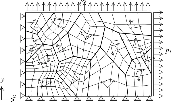
The correlation length is estimated on the stress field of a 0.4 [mm] by 0.28 [mm] size finite element model, Fig. 1. The model is composed of 212 crystal grains (bold lines) with randomly oriented crystal lattices. Orientations of crystal lattices are shown with local coordinate systems x’-y’. Crystal grains are generated with the Voronoi tesselation. For clarity reasons an example with only 14 crystal grains is shown in Fig. 1.

p

1

x

y

y'_x'

x'y' x' y' x' y' x'y' x' y' x' y' x' y' x' y' x' y' x' y'

p

2 x' y' x' y' x' y'

Fig. 1: Finite element model of a polycrystalline aggregate with orientations of crystal lattices, loading and boundary conditions

Each crystal grain (monocrystal) is assumed to behave as a continuum. Within the crystal grain all finite elements have the same material orientations. However, material orientations vary between different crystal grains. Anisotropical elasticity and crystal plasticity [7-9] material models were applied. Crystal plasticity model assumes plastic deformation by simple shear on the specified set of slip planes. The slip planes are essentially defined by the random orientations of crystal lattices, which differ among the grains. Material parameters for reactor pressure vessel steel 22 NiMoCr 3 7 were used. This steel has bainitic microstructure with body-centered cubic crystal lattice and rather pronounced orthotropic elasticity. The material parameters used in the model are described in [10].

CORRELATION LENGTH

The cumputational effort needed for the calculation of the stress/strain fields using the crystal plasticity material model is quite large, limiting the size of the models to approximately 0.40 [mm] by 0.28 [mm]. The numerical effort could be reduced if only the essential inhomogenities were taken into the account. One way of estimating essential inhomogenities is to calculate the domain of influence of crystal grains. In this work the correlation length is taken as a measure of the domain of influence of the individual crystal grains.

The autocorrelation function Rxx(l1,l2) of a random process x(l) is defined with the eq. (1), where E[] represents

mathematical expectation and _{( ) ( )}

2 1xl

l x

f

joint probability density function. The covariance function Kxx(l1,l2) of a

random process x(l) is defined with the eq. (2) and can be expressed using the autocorrelation function, eq. (3).

( )

l

1

,

l

2

=

E

[

x

( ) ( )

l

1

⋅

x

l

2

]

=

∫∫

x

1

⋅

x

2

⋅

f

( ) ( )1 2

(

x

1

,

x

2

)

⋅

dx

1

⋅

dx

2

R

_{xx xl xl} (1)

( )

l

₁

,

l

₂

E

[

(

x

(

l

₁

)

E

[

x

(

l

₁

)

]

)

(

x

(

l

₂

)

E

[

x

(

l

₂

)

]

)

]

K

_xx

=

−

⋅

−

(2)

( )

l

1

,

l

2

R

( )

l

1

,

l

2

E

[ ]

x

( )

l

1

E

[

x

( )

l

2

]

K

_xx

=

_xx

−

⋅

(3)

For stationary random processes the joint probability density function _{( ) ( )}

2 1xl

l x

f

depends only upon the difference l2-l1.

Consequently, the autocorrelation and covariance functions also depend only upon the difference l2-l1. If in addition to

the stationarity, the average value of the random process is zero, then the autocorrelation and covariance functions of the process involved are equal, expressions (4) and (5).

( )

l

1

,

l

2

R

(

0

,

l

2

l

1

)

R

(

l

2

l

1

)

R

( )

l

,

l

l

2

l

1

R

_xx

=

_xx

−

=

_xx

−

=

_xx

=

−

(4)

( )

l

K

(

l

l

)

R

( )

l

E

[ ]

x

( )

E

[

x

(

l

l

)

]

R

( )

l

K

_xx

=

_xx

−

=

_xx

−

⋅

−

=

_xx

=

=

3

1

42

43

2

1

0 1 2 0 1

2

0

(5)

( )

l

K

( )

e

( )

l

K

_xx

=

_xx

₀

⋅

−l /λ

⋅

_cos

_ω

⋅

(6)

l

Kxx (l) 0

K

xx

(0)

K

xx

(0)/e

λ

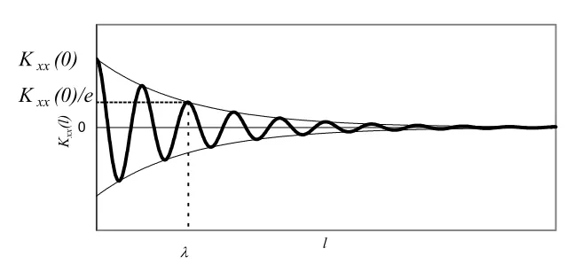
Fig. 2: Correlation length λ definition

Let us assume that we have a vector of data g for which we want do determine the correlation length. First the autocorrelation function is estimated using discrete correlation theorem, eq. (7). In eq. (7) symbol Gk presents discrete

Fourier transformation of vector g while symbol * stands for complex conjugation. First we calculate the discrete Fourier transform of vector g to obtain Gk. Next we multiply, index by index, the vector Gk with the Gk*. Finally we

calculate the inverse Fourier transform of the product Gk Gk* to determine the autocorrelation function. Correlation

length is calculated from the envelope of the autocorrelation function. Instantaneous envelope of a function f(t) is defined with the eq. (8), where H(t) presents the Hilbert transform, eq. (9), of function f(t).

( )

,

_⇔

_G

_G

*

,

_k

₌

0

,

1

,

2

,

_length

(

_G

)

₋

1

Autocorr

g

g

_{j k k}

_K

(7)

( ) (

) (

2

)

2

)

(

)

(

t

H

t

f

t

A

=

+

(8)

( )

_∫

+∞

₍

_{) ( )}

∞

−

⋅

−

⋅

⋅

=

τ

τ

τ

π

t

f

d

t

H

1

(9)

The correlation length is calculated from the equivalent (Mises) stress, eq. (10), determined for every Gaussian integration point of the finite elements. For the correlation length calculation the stress is assumed to be a random variable.

(

) (

)

(

)

[

2 2 2 2 2 2

]

6

6

6

2

1

zx yz xy x

z z

y y

x

eq

σ

σ

σ

σ

σ

σ

τ

τ

τ

σ

=

−

+

−

+

−

+

+

+

(10)

ESTIMATION ISSUES

Since stress is a two-dimensional variable, a vector of data for the correlation length calculation has to be extracted. This raises several issues, one of them beeing the method of obtaining the data for the vector g, eq. (7). The data (Mises stress) in the vector g has to be spaced equally, however the Gaussian points are not equally spaced. Therefore the Mises stress for given coordinates has to be calculated from the appropriate finite element. For an 8-node finite quadratic element this can be quite cumbersome since conversion from physical to natural coordinates and back is needed. In this work the alternative approach is used. Shepard’s quadratic two-dimensional interpolation on a scattered data set (stresses) [11] is applied to obtain the values of the stresses in the equally spaced points on the direction line within the search radius (bold line in the Fig 3).

At the end, the search radius R determining the length of vector g has to be considered. If a small search radius R is chosen it is possible that the vector g will contain unsufficient information on the stress field for a meaningfull estimation of the correlation length. On the other hand when a large search radius R is chosen, the vector g contains stress information from a larger ‘area’ and may not be a representative measure of a local domain of influence of a crystal grain. In addition, when a large search radius R is used a part of the vector g is much more prone to falling outside of the model area. For the points of the vector g outside of the model area stresses are assumed to be zero.

x y

p2

p1

selected direction α selected integration

point

Search area

Search radius R

α

The length of the vector

Fig 3: The length 2R and direction α of the vector g for calculating the correlation length

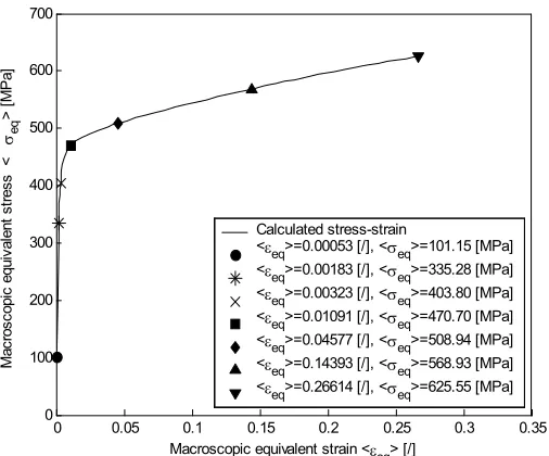
0 0.05 0.1 0.15 0.2 0.25 0.3 0.35 0 100 200 300 400 500 600 700

Macroscopic equivalent strain <ε_eq> [/]

M ac ros copi c equi val ent s tr es s < σeq > [M P a] Calculated stress-strain

<ε_eq>=0.00053 [/], <σ_eq>=101.15 [MPa] <ε_eq>=0.00183 [/], <σ_eq>=335.28 [MPa] <ε_eq>=0.00323 [/], <σ_eq>=403.80 [MPa] <ε_eq>=0.01091 [/], <σ_eq>=470.70 [MPa] <ε_eq>=0.04577 [/], <σ_eq>=508.94 [MPa] <ε_eq>=0.14393 [/], <σ_eq>=568.93 [MPa] <ε_eq>=0.26614 [/], <σ_eq>=625.55 [MPa]

Fig. 4: Macroscopic strain/stress of the model for which correlatin lengths are presented

Correlation lengths were calculated for all the steps and increments used by ABAQUS for obtaining the strain/stress fields. However, only 7 cases, refering to 7 different macroscopic strains/stresses on a tensile stress curve (shown in Fig. 4) are presented in this work. Macroscopic equivalent stress <σeq> and macroscopic equivalent strain

<εeq> were calculated as

∫

=

V eq

eq

dV

V

σ

σ

1

,

=

∫

V eq

eq

dV

V

ε

ε

1

, (11)

(

) (

)

(

)

[

]

2

1 2 2 2 2 2 2

6

6

6

3

2

zx yz xy x z z y y x

eq

ε

ε

ε

ε

ε

ε

ε

ε

ε

where σeq stands for the equivalent stress, eq. (10), εeq for the equivalent strain, eq. (12), and V for volume of

polycrystalline aggregate.

RESULTS AND DISCUSSION

In the presented work two different search radiuses were used, corresponding to average crystal grain size (0.23 [mm]) and twice the average crystal grain size (0.46 [mm]). For the purpose of brevity the results associated with the search radius of the average crystal grain size will be denoted as case a) while the results associated with twice the average crystal grain size will be denoted as case b).

Correlation lengths for the presented cases are listed in Table 1. One can see that correlation lengths are higher for the case b). Since in theory the vector g should have infinite length for calculating the correlation length, the change in results is expected. However, above certain length of the vector g the calculated correlation lengths should not change significantly. Comparing the results in Table 1 it is reasonable to conclude that this correlation length is still larger than the length of the search radius of the case b) (R=0.046 [mm]). The correlation length should therefore be calculated with an even larger search radius R. This would require a significantly larger finite element model. At this point this is beyond our computational capabilities.

Table 1: Correlation length values

Correlation length [mm], case a),

R=0.023 [mm] Correlation length [mm], case b),R=0.046 [mm]

<εeq> [/] <σeq> [MPa]

Minimal Maximal Average Minimal Maximal Average

0.00053 101.15 0.00236 0.03564 0.01704 0.00370 0.06505 0.02731

0.00183 335.28 0.00237 0.03514 0.01691 0.00348 0.06495 0.02728

0.00323 403.80 0.00209 0.03440 0.01634 0.00504 0.06127 0.02686

0.01091 470.70 0.00211 0.03331 0.01578 0.00277 0.06160 0.02652

0.04577 508.94 0.00259 0.03458 0.01574 0.00283 0.06147 0.02643

0.14393 568.93 0.00188 0.03306 0.01552 0.00292 0.06153 0.02544

0.26614 625.55 0.00136 0.03244 0.01497 0.00375 0.05499 0.02149

The applied load also has an influence on correlation lengths. As long as resulting strain/stress values increse proportionally, values of covariance functions also increase. However, this has no effect on calculated correlation lengths since the correlation length is defined as a length for which the starting value of the envelope of the covariance function decreases by a factor of e=2.718…As a result the correlation lengths do not change as long as the strain/stress field is in the elastic region. The maximal correlation length in elasticity (<εeq>=0.00053 [/] and <σeq>=101.15 [MPa])

for case b) is λmax=0.06505 [mm], corresponding to 2.83 the average size of a crystal grain. For the same case the

average value of the correlation length is λave=0.02731 [mm], which is 18 % larger than the average crystal grain size.

For the case a) the maximal correlation length is λmax=0.03564 [mm], corresponding to 1.55 the average size of a crystal

grain. The average value of the correlation length is λave=0.01704 [mm]–lower than the average crystal grain size.

At <εeq>=0.00183 [/] and <σeq>=335.28 [MPa] parts of the finite element model exhibit plastic deformations.

This non-proportionally changes the strain/stress field resulting in a change of the correlation lengths. For this increment the majority of the stress field is proportional to the stress field of the previous increment. As a result average the correlation lengths are very similar to the average correlation lengths of the previous increment, Table 1.

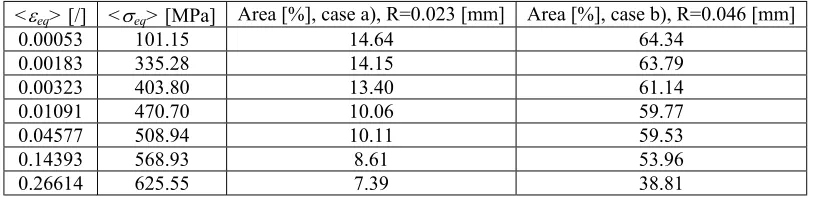
Table 2: Area of the model with correlation lengths larger than the average crystal grain size(0.023 [mm])

<εeq> [/] <σeq> [MPa] Area [%], case a), R=0.023 [mm] Area [%], case b), R=0.046 [mm]

0.00053 101.15 14.64 64.34

0.00183 335.28 14.15 63.79

0.00323 403.80 13.40 61.14

0.01091 470.70 10.06 59.77

0.04577 508.94 10.11 59.53

0.14393 568.93 8.61 53.96

0.26614 625.55 7.39 38.81

elastic region

plastic regi

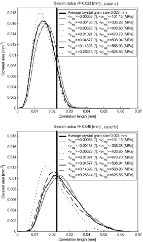
With the increase of the macroscopic equivalent strain/stress beyond the elastic (proportional) limit the strain/stress fields change significantly. More and more finite element model exhibit plastic deformations and as a result the correlation lengths decrease. This can be seen as a reduction of the model area that is covered by correlation lengths larger than the average crystal grain size, Table 2. The reduction is most evident between the last two calculation increments. The histograms of model area with the regard to the correlation length are shown on Fig. 5. One can see that with the increase of the macroscopic equivalent strain/stress the lines move to the left-a consequence of the average correlation lengths decrease. For the case a) the area distribution lines are similar to the Gaussian distribution while for the case b) the area distribution lines are closer to a χ2 _{distribution. The reduction of correlation lengths suggests that} the stresses in the vector g become increasingly more random as the load and the macroscopic equivalent stress increase. Since the correlation length is taken as a measure of the domain of influence of crystal grains we can conclude that the domain of influence of crystal grains reduces as the macroscopic equivalent stress/strain increase.

0 0.01 0.02 0.03 0.04 0.05 0.06 0.07

0 0.002 0.004 0.006 0.008 0.01 0.012 0.014 0.016 0.018

Correlation length [mm]

C

ov

ered

are

a

[m

m

2]

Search radius R=0.023 [mm]

Average crystal grain size 0.023 mm <ε_eq>=0.00053 [/], <σ_eq>=101.15 [MPa] <ε_eq>=0.00183 [/], <σ_eq>=335.28 [MPa] <ε_eq>=0.00323 [/], <σ_eq>=403.80 [MPa] <ε_eq>=0.01091 [/], <σ_eq>=470.70 [MPa] <ε_eq>=0.04577 [/], <σ_eq>=508.94 [MPa] <ε_eq>=0.14393 [/], <σ_eq>=568.93 [MPa] <ε_eq>=0.26614 [/], <σ_eq>=625.55 [MPa]

0 0.01 0.02 0.03 0.04 0.05 0.06 0.07

0 0.002 0.004 0.006 0.008 0.01 0.012 0.014 0.016 0.018

Correlation length [mm]

C

ov

ered

are

a

[m

m

2]

Search radius R=0.046 [mm]

Average crystal grain size 0.023 mm <ε_eq>=0.00053 [/], <σ_eq>=101.15 [MPa] <ε_eq>=0.00183 [/], <σ_eq>=335.28 [MPa] <ε_eq>=0.00323 [/], <σ_eq>=403.80 [MPa] <ε_eq>=0.01091 [/], <σ_eq>=470.70 [MPa] <ε_eq>=0.04577 [/], <σ_eq>=508.94 [MPa] <ε_eq>=0.14393 [/], <σ_eq>=568.93 [MPa] <ε_eq>=0.26614 [/], <σ_eq>=625.55 [MPa]

Fig. 5: Histogram of model area with regard to the correlation length , case a)

Fig. 8: Correlation length for the <εeq>=0.04577 [/] and <σeq>=508.94 [MPa]. Case b), R=0.046 [mm]

Fig. 6 shows Mises stresses for the equivalent strain <εeq>=0.04577 [/] and stress <σeq>=508.94 [MPa]. Crystal

boundaries are plotted with white lines. On the basis of these stresses the correlation lengths were calculated with the search radiuses of R=0.023 [mm]-case a)- and 0.046 [mm]-case b). These correlation lengths are shown on Fig. 7 and Fig. 8. One can see that correlation lengths for the case b) are higher. The areas of higher correlation length values for both cases are most often inside the grains, sometimes spreading over several grains. In a few cases the areas of higher correlation length values seem to concentrate on the grain boundaries. For the case b) the regions of high correlation values can be seen at the model boundaries. This is due to the 2D interpolation of the Mises stresses in the border region where there is a lack of data on the Mises stresses outside the model boundaries.

CONCLUSIONS

The estimation of a domain of influence of a crystal grain has been presented. The domain of influence has been estimated with the correlation length averaged over several directions.

should be relatively small. However, if the search area is too small insufficient stress information may be captured. In the presented work search radiuses equal to the average crystal grain size (0.023 [mm]) and twice the average crystal grain size (0.046 [mm]) have been used. It has been shown, that correlation lengths are higher for the larger search radius.

The results obtained show that on the average and for the search radius equal to twice the average crystal grain size the correlation length is slightly larger than the average crystal grain size. For the elastic aggregate the maximal correlation length value is λmax=0.06505 [mm], corresponding to roughly 2.8x the average size of a crystal grain. The average value of the correlation length is λave=0.02731 [mm], slightly above the average crystal grain size. With the increase of the macroscopic strain/stress the correlation lengths decrease. For the fully plastic aggregate the average correlation length was determined to be λave=0.02149 [mm], slightly bellow the average crystal grain size.

REFERENCES

1. Aurenhammer, F., "Voronoi Diagrams-A Survey of a Fundamental Geometric Data Structure", ACM Computing Surveys, 23 (3), pp. 345-405, 1991.

2. Kovač, M., Simonovski, I., and Cizelj, L., "Estimating Minimum Polycrystalline Aggregate Size for Macroscopic Material Homogeneity", Proceedings of the International Conference Nuclear Energy for New Europe, article in press.

3. Chakraborty, S. and Dey, S. S., "Stochastic Finite Element Method for Spatial Distribution of Material Properties and External Loading", Computers & Structures, 55 (1), pp. 41-45, 1995.

4. Schenk, C. A. and Schuëller, I. R., "Buckling analysis of cylindrical shells with random geometric imperfections",

International Journal of Non-Linear Mechanics, article in press.

5. Zheng, R. and Ellingwood, B. R., "Stochastic fatigue growth in steel structures subject to random loading",

Structural Safety, 20 (4), pp. 303-323, 1998.

6. ABAQUS 6.3-1/Standard", Hibbit, Karlsson & Sorensen Inc., 2002.

7. Watanabe, O., Zbib, H. M., and Takenouchi, E., "Crystal Plasticity: Micro-Shear Banding in Polycrystals using Voronoi Tessellation", International Journal of Plasticity, 14 (8), pp. 771-778, 1998.

8. Kovač, M., Cizelj, L., and Simonovski, I., "Mezoscopic approach to elastic-plastic behavior of polycrystalline material", to be submitted.

9. Kovač, M., "Influence of Microstructure on Development of Large Deformations in Reactor Pressure Vessel Steel", draft of Ph.D. thesis.

10. Kovač, M., Cizelj, L., and Simonovski, I., "Modeling Elasto-Plastic Behavior Of Polycrystalline Grain Structure Of Steels At Mesoscopic Level", Vejvoda, S., Structural Mechanics in Reactor Technology (SMiRT 17), 2003. 11. Renka, R. J., "Quadratic Shepard Method for Bivariate Interpolation of Scattered Data", ACM Transactions on