ABSTRACT
MASON, SARAH BETH. Conjugacy Classes of Maximal k-split Tori Invariant Under an Involution of SL(n,k). (Under the direction of Dr. Aloysius Helminck.)
Given an involutionθand a reductive algebraic groupG, we define a symmetric space as the spaceG/H, whereH is the fixed point group ofθ. One can extend the applications of symmetric spaces to symmetric k-varieties over an arbitrary field k. To study the representation theory of symmetric k-varieties, it is important to first understand their structure. The action of minimal parabolic k-subgroups on symmetric k-varieties helps in identifying the structure of these symmetrick-varieties. Maximal k-split tori invariant under an involution are of fundamental importance in the characterization of minimal parabolic k-subgroups acting on symmetric k-varieties. In this dissertation, symmetric k-varieties for the special linear group SL(n, k) are considered and a classification of standard tori is given. From the standard tori, one can study the H- and Hk-conjugacy
©Copyright 2015 by Sarah Beth Mason
Conjugacy Classes of Maximal k-split Tori Invariant Under an Involution of SL(n,k)
by
Sarah Beth Mason
A dissertation submitted to the Graduate Faculty of North Carolina State University
in partial fulfillment of the requirements for the Degree of
Doctor of Philosophy
Mathematics
Raleigh, North Carolina 2015
APPROVED BY:
Dr. Ernest Stitzinger Dr. Tom Lada
Dr. Bojko Bakalov Dr. Aloysius Helminck
DEDICATION
BIOGRAPHY
TABLE OF CONTENTS
LIST OF TABLES . . . vi
LIST OF FIGURES . . . vii
Chapter 1 Introduction . . . 1
1.1 Symmetric Spaces . . . 1
1.2 Orbits of Parabolic Subgroups on Symmetric Spaces . . . 3
1.3 Hk-conjugacy classes of θ-stable maximal k-split tori . . . 5
1.4 Summary of Results for SL(2, k) . . . 8
1.4.3 Summary of Results for SL(n, k) . . . 9
Chapter 2 Preliminaries . . . 12
2.1 Preliminaries . . . 12
2.2 Generalized Symmetric Spaces . . . 14
2.3 Algebraically Closed vs. Non-algebraically Closed . . . 18
2.4 Lie Algebras . . . 21
2.5 Pk\Gk/Hk . . . 22
Chapter 3 Standard Tori . . . 24
3.1 Standard k-split tori . . . 24
3.2 Standard Quasi k-split tori . . . 28
3.3 Standard H-Quasi k-split tori . . . 31
Chapter 4 SL(2, k) . . . 32
4.1 Introduction to SL(2, k) . . . 32
4.1.2 k =C . . . 33
4.1.4 k =R . . . 34
4.1.6 k =Fp . . . 34
4.2 Orbit Decompositions of SL(2, k) . . . 35
Chapter 5 Building the Poset of Tori . . . 37
5.1 Computing the maximal (θ, k)-split tori . . . 37
5.2 Hk-conjugacy classes of (θ, k)-split maximal tori . . . 40
5.3 Restricting θ to Gα . . . 41
Chapter 6 (θ, k)-singular roots of Involutions of SL(n, k) . . . 46
6.1 Outer Involutions . . . 46
6.1.1 (AT)−1 . . . 46
6.1.7 InnMi(A
T)−1 . . . . 52
6.2 Inner Involutions . . . 56
6.2.1 Inn(In−i,i) . . . 56
6.2.5 Inn(Ln,−1) . . . 61
Chapter 7 Conjugacy Classes of Maximal θ-stable, k-split Tori . . . 63
7.1 Quasi k-split tori . . . 63
7.2 Hk-Conjugacy . . . 64
LIST OF TABLES
Table 6.1 Outer Involutions of G overk = ¯k, R and Fp with p6= 2. . . 47
Table 6.2 Outer Involutions of G overk =Q2 . . . 48
Table 6.3 Outer Involutions of SL(n,Qp) (p6= 2) . . . 49
LIST OF FIGURES
Figure 1.1 Poset of Hk-conjugacy classes of θ-stable maximalk-split tori . . . . 6
Figure 1.2 Posets of tori related to G= SL(4,C) withθ(A) = (AT)−1 . . . . 7
Figure 2.1 Illustration of k-split and θ-split parts of tori . . . 13
Figure 5.1 Flipping one dimension of a torus . . . 45
Figure 6.1 Standard Poset for G= SL(4,C), θ = (AT)−1 . . . . 50
Figure 6.2 Poset of standard tori related toG= SL(4,R) withθ(A) = InnM1(A T)−1 55 Figure 6.3 Poset of standard tori for SL(4, k) and θ = Inn(I2,2) . . . 61
Figure 7.1 Poset of standard tori forSL(3,R) . . . 64
Figure 7.2 Poset of quasi k-split tori forSL(3,R) . . . 65
Figure 7.3 Graph demonstrating how to check for conjugacy . . . 66
Figure 7.4 Poset of Standard tori for SL(3,F3, θ = InnM1(A T)−1 . . . . 68
Figure 7.5 Poset of Hk-conjugacy classes of θ-stable, maximal k-split tori for SL(3,F3, θ= InnM1(A T)−1 . . . . 69
Figure 7.6 Poset of standard θ-stable, maximal k-split tori for SL(4,C), θ(X) = (XT)−1 . . . . 70
Chapter 1
Introduction
1.1
Symmetric Spaces
Given an involution θ and a reductive algebraic group G, we define a symmetric space
as the space G/H, where H is the fixed point group of θ. A symmetric space is also known as a symmetric variety. Symmetric spaces were originally studied by Cartan and arose in the context of Riemannian manifolds and Lie groups. The globally Riemannian symmetric spaces of differential geometry are a special case of the algebraic definition common in Lie theory.
One can also consider a more generalized version of a symmetric space. When consid-ering a symmetric space over a non-algebraically closed field k, we call this a symmetric
k-variety, and it is defined by Gk/Hk, where Gk and Hk are the k-rational points of G
and H, respectively. Real symmetric k-varieties are also called real reductive symmetric
spaces. The p-adic symmetric k-varieties are also known as reductive p-adic symmetric
spaces or as simply p-adic symmetric spaces.
Symmetric k-varieties over fields other than the real numbers occur in a number of areas of mathematics. These areas include representation theory (see [6], [37] and [38], geometry ([10],[11],[3]), singularity theory ([28],[24]), the study of character sheaves ([14], [29]), and the study of cohomology of arithmetic subgroups ([36]). These symmetric k-varieties are most well known in the area of representation theory.
Example 1.1.1. Let Mn(k) denote the set of n×n matrices with entries in k. Then
is the general linear group. Let G = GL(n, k) and define an involution θ : G → G by θ(g) = (gT)−1. Then H ={g ∈ G|gT =g−1}, the set of n×n orthogonal matrices.
The quotient G/H is then contained within the set of symmetric matrices, giving the motivation for the name symmetric space. If k = ¯k, then G/H is the set of symmetric matrices. Whenk 6= ¯k, then the extended symmetric space ˜Q={A∈GL(n, k)|θ(A) = A−1} is the set of symmetric matrices.
Representations associated with real reductive symmetric spaces have been studied by many people over the past few decades. Much of the early work was done by Harish-Chandra. Symmetric k-varieties were first introduced in the late 1980’s as a way of generalizing the concept of these real reductive symmetric spaces to similar spaces over the p-adic numbers and as a way to study the representations that are associated with these spaces. A number of interesting results have arisen from this research (see [17], [27], [33]). Another case of interest is the representations associated with symmetrick-varieties defined over a finite field (see [29] and [14]).
Expanding on Harish-Chandra’s ideas, the representation theory for the general real reductive symmetric spaces has been carried out by a number of mathematicians including Flensted-Jensen, ¯Oshima, Sekiguchi, Matsuki, Brylinski, Delorme, Schlichtkrul, and van den Ban (see [5], [9], [12],[13], [15], [31], [32]).
ForQp, thep-adic numbers, it is natural to study the harmonic analysis of thesep-adic
symmetric spaces. The main aim of harmonic analysis is to decompose unitary represen-tations as explicitly as possible into irreducible components, which is called finding the
Plancherel decomposition. Most of the representations occurring in this decomposition
1.2
Orbits of Parabolic Subgroups
on Symmetric Spaces
There are several ways of classifying the orbits of a minimal parabolick-subgroup Pk on
a symmetric k-variety. One way of classifying these orbits is to consider the Pk-orbits
acting on the symmetric k-variety Gk/Hk by a process called θ-twisted conjugation.
For x, g ∈ Gk, we define g ∗x := gxθ(g)−1. Another way of viewing these orbits is to
identify Gk/Pk with the set of parabolic k-subgroups of G that are Gk-conjugate with
P, i.e. Gk/Pk ={xP x−1 | x ∈ Gk}, and look at the Hk-orbits on this. Here Hk acts by
conjugation. Lastly, we can consider these orbits as the setPk\Gk/Hk of (Pk, Hk)-double
cosets in Gk. This last characterization is the same as the set of Pk ×Hk-orbits on the
setGk.
When we have that k=k, we use a Borel subgroupB in place of a minimal parabolic k-subgroup, because in the case of algebraic closure we have that P =B. For this case, these orbits were characterized by Springer [35]. Several characterizations of the double cosets B \ G/H were proven by Springer, including the orbits of H, B, and B ×H. For details, see [35]. For algebraically closed k and P a general parabolic subgroup, these orbits were characterized by Brion and Helminck in [8] and [21]. For k = R and P a minimal parabolic k-subgroup, characterizations were given by Matsuki [30] and Rossmann [34]. For general fields, these orbits were characterized by Helminck and Wang [22].
Let Pk be a minimal parabolic k-subgroup of G. The double coset Pk\Gk/Hk has
been characterized in several ways by Helminck and Wang [22], including the orbits of Hk, Pk, and Pk×Hk.
We will first consider the Hk-orbits on Gk/Pk. If we let A be a torus of Gk, then
we can denote by NGk(A) the normalizer of A in Gk, ZGk(A) denotes the centralizer
of A in Gk, WGk(A) = NGk(A)/ZGk(A) the Weyl group of A in Gk, and WHk(A) =
NHk(A)/ZHk(A) = {w ∈ WGk(A) | w has a representative in NHk(A)}, the Weyl group
of A inHk. All of the above sets are θ-stable if A is θ-stable.
Let A0 be a θ-stable maximal k-split torus of Gk which is contained in the minimal
parabolic k-subgroup P0. Then we will denote by Ck the set of pairs of (P0, A0). Pk will
be the space of all minimal parabolic k-subgroups of G. The fixed point group Hk acts
byHk\Ck (respectivelyHk\Pk ).
The Hk-orbits in Ck can be broken up into two parts. We can first consider the Hk
-conjugacy classes ofθ-stable maximalk-split tori inGk. For eachθ-stable maximalk-split
torus that is a representative of these conjugacy classes, we can determine the minimal parabolick-subgroups containing this torus that are notHk-conjugate. Thus, if we define
the set {Ai | i ∈ I} as the set of representatives of the Hk-conjugacy classes of θ-stable
maximal k-split tori in Gk, then the Hk-orbits in Ck can be identified with the union of
Weyl group quotients S
i∈IWGk(Ai)/WHk(Ai).
For thePk-orbits, we identifyGk/HkwithQk ={gθ(g)−1 |g ∈Gk}.Pkacts onQkby
the θ-twisted action previously described. We will denote the set of θ-twisted Pk-orbits
onQk byPk\Qk.
In the characterization of thePk×Hk-orbits inGk, letAbe aθ-stable maximalk-split
torus of Pk and Vk ={x∈Gk |τ(x)∈NGk(A)}, where τ(x) is defined as follows.
τ(x) =xθ(x)−1 The groupZGk(A)×Hkacts onVkby (x, z)·y=xyz
−1,(x, z)∈Z
Gk(A)×Hk, y ∈Vk.
LetVk be the set of (ZGk(A)×Hk)-orbits on Vk.
Theorem 1.2.1. [22] Let P be a minimal parabolic k-subgroup of G and let {Ai |i∈I}
be representatives of theHk-conjugacy classes ofθ-stable maximalk-split tori inGk. Then
Pk\Gk/Hk 'Hk\Pk '
[
Ai∈I
WGk(Ai)/WHk(Ai)'Hk\Ck'Pk\Qk 'Vk.
From the previous theorem, we can see that there are several ways to classify the double cosetsPk\Gk/Hk. Throughout this thesis, we will be interested in the classification
Pk\Gk/Hk '
[
Ai∈I
WGk(Ai)/WHk(Ai).
This classificiation will help us in studying the orbits of minimal parabolick-subgroups acting on the symmetrick-variety. From this classification, we see that in order to classify the double cosetPk\Gk/Hk, we will first need to classify the set ofHk-conjugacy classes
ofθ-stable, maximalk-split tori. This will give us the set{Ai |i∈I}. Once we have done
k-split tori representative Ai.
In an algebraically closed field, i.e. k = ¯k, we have the double cosets B \ G/H. When considering G over a non-algebraically closed field, we look at minimal parabolic k-subgroups instead of Borels and we get Pk \Gk/Hk. One method of classifying these
double cosets is to considerP \G/H and determining how the algebraically closed orbits break up over thek-rational points. An alternate method is to instead reverse this process via an embedding mapPk\Gk/Hk,→P\G/H which we call generalized complexification.
The surjectivity of the generalized complexification map is then equivalent to all orbits over the algebraic closure contributing to the k-orbits. Given a group N, k-rank(N) denotes the dimension of a maximal k-split torus of N. When the group Gis k-split we have a characterization of the surjectivity:
Theorem 1.2.2. [26] LetG be a k-split group, H the set of fixed points of an involution
θ and P a minimal parabolic k-subgroup. Then the generalized complexification map
ϕ:Pk\Gk/Hk →P \G/H, ϕ(PkxHk) = P xH
is surjective if and only if k-rank(H) = k-rank(G).
This embedding process will be the motivation for considering theH-conjugacy classes of θ-stable, maximal k-split tori as well as the Hk-conjugacy classes ofθ-stable, maximal
k-split tori.
1.3
H
k-conjugacy classes of
θ
-stable maximal
k
-split
tori
The classification that we are interested in centers around tori, so we will use the following definitions and results. If we have a torus T of G that is defined over the field k, then there are subtori Ta andTs ofT, whereTa is the largest anisotropic subtorus of T andTs
is the largest k-split subtorus of T defined over k. We have thatT =Ta·Ts and Ta∩Ts
is finite.
Given an involution θ of G, we have similar definitions and results for θ-stable tori. Let T be a maximal k-split torus. We call T θ-stable if θ(T) = (T). If we let T+ ={t ∈
T+∩T− is finite. We call the torusT− θ-split. A torusT is called (θ, k)-split if it is both
k-split and θ-split.
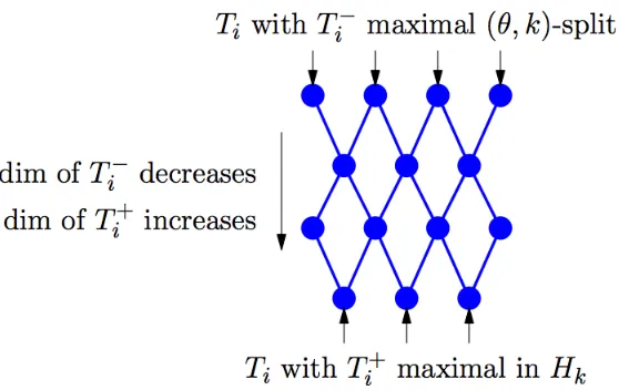
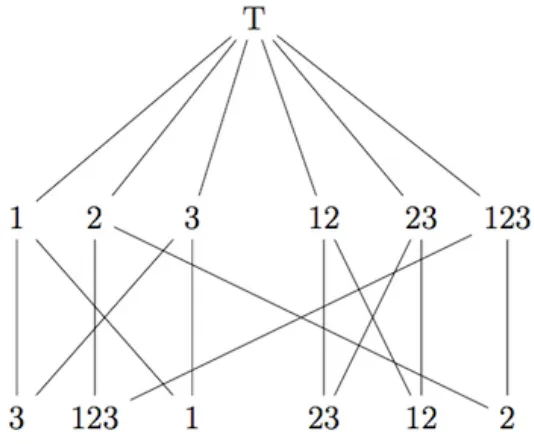
Figure 1.1: The poset of Hk-conjugacy classes of θ-stable maximal k-split tori
As we are classifying the Hk-conjugacy classes of θ-stable, maximal k-split tori, we
will obtain a poset of tori. Each node in the poset will represent one of theHk-conjugacy
classes of θ-stable, maximal k-split tori. As we have stated previously, each of these representatives Ti can be written as the product of two subtori, Ti =Ti+T
−
i . As we look
across each level of the poset, the dimension of Ti+ for each torus Ti on that level will
be equivalent. The same is true for the dimension of Ti− across each level of the poset. We construct the poset in such a way that the top level has tori with a maximal θ-split part, i.e. T− is maximal. Also, we will have the tori with a maximal T+ part at the bottom level of the poset. As we move down the poset, we decrease the dimension of the θ-split portion of the torus by one and increase the dimension of the T+ part by one. A representation of this poset can be seen in Figure 1.1.
Once we have constructed the poset of Hk-conjugacy classes of θ-stable, maximal
k-split tori, we can get a second poset by expanding each node. Our motivation for creating the first poset is to classify the Weyl group quotientsWGk(Ti)/WHk(Ti). Since each node
represents one of ourTi’s, we can expand the poset to give us this quotient. The number
of nodes in this second lattice will give us|Pk\Gk/Hk |. Additionally, the lines connecting
Figure 1.2: Posets of tori related to G= SL(4,C) with θ(A) = (AT)−1
Example 1.3.1. Let G = SL(4,C) with θ(A) = (AT)−1. Then the first poset has three levels with one Hk-conjugacy class of θ-stable k-split tori in each level. In the top and
bottom levels, we have that | WGk(Ti)/WHk(Ti) |= 2. Then |Pk\Gk/Hk | = 4. This is
shown graphically in Figure 1.2.
In order to determine the poset of Hk-conjugacy classes of θ-stable, maximal k-split
tori and the expansion at each node to WGk(Ti)/WHk(Ti), we will need to consider each
algebraic group G and its involutions individually. Throughout this thesis, we will be considering the groupG= SL(n, k) and the involutions associated with it. We will break up our problem into various subproblems in order to help classify Pk\Gk/Hk.
1. Classify the Hk-conjugacy classes of the maximal (θ, k)-split tori.
2. Classify the Hk-conjugacy classes of maximal k-split tori containing a maximal
(θ, k)-split torus. These tori are θ-stable and the number of conjugacy classes will tell us the number of nodes in the top level of the first poset, whose nodes correspond to the Hk-conjugacy classes of θ-stable, maximal k-split tori.
3. Determine the maximal k-split tori in Hk and classify the Hk-conjugacy classes of
θ-stable maximal k-split tori which contain a maximal k-split torus in Hk. This
will give us the bottom level of the first poset, whose nodes are the Hk-conjugacy
classes of θ-stable maximal k-split tori.
4. Classify the Hk-conjugacy classes of θ-stable maximal k-split tori. This is where
we will determine all of the middle levels of the first poset, whose nodes are the Hk-conjugacy classes of θ-stable maximal k-split tori.
of standard tori and see how this poset collapses down underH-conjugacy and then how it expands when we consider Hk-conjugacy.
Once the poset of Hk-conjugacy classes of θ-stable, maximal k-split tori has been
constructed, we are able to started classifying the Weyl group quotientsWGk(Ti)/WHk(Ti)
in order to characterize the double cosets Pk\Gk/Hk.
1.4
Summary of Results for
SL(2
, k
)
When looking to classify the Hk-conjugacy classes of θ-stable, maximal k-split tori for
G= SL(n, k), it is natural to start with the casen = 2. For G = SL(2, k), we have that tori ofGare one-dimensional; thus,Ti =Ti+ orTi =Ti−. There are at most two levels to
the poset for SL(2, k).
Remark 1.4.1. SL(2, k) is a k-split group. This means that SL(2, k) contains a
maxi-mal torus that is also maximaxi-mal k-split, namely T = {diagonal matrices} = {diag} = a 0
0 a−1
!
. In this case, minimal parabolick-subgroups are also Borel subgroups. Thus, if we let B be a Borel subgroup, T ⊆B, the classification of Bk\Gk/Hk is identical to
the classification of Pk\Gk/Hk.
The classification of involutions of SL(2, k) is given by Helminck and Wu. They show all involutions come from bilinear forms. In particular, we have the following theorem for involutions of SL(2, k). Note that θ(X) = InnA(X) = A−1XA for any X ∈G.
Theorem 4.1.1 [23] The number of isomorphy classes of involutions over G= SL(2, k)
equals the order of k∗/(k∗)2. Furthermore, the involutions over G are of the form θ =
Inn (0 1
m0) for all m ∈ k∗/(k∗)2. Additionally, if m and q are in the same square class,
then Inn (0 1
m0) is isomorphic to the involution Inn 0 1q0
.
Since all involutions of SL(2, k) come from bilinear forms, the orbits of minimal parabolick-subgroups acting on the symmetrick-variety related to the involution can be classified using quadratic forms.
A summary of the main results for SL(2, k) is found in the following theorem. Note that we use ¯m to denote the entire square class of mand we use m∈k∗/(k∗)2 to denote
Theorem 1.4.2. [1] Let Gk = SL(2, k) and let θ = Inn (m0 10).
1. Hk is k-anisotropic if and only if m 6∈ ¯1. If m ∈ ¯1, then Hk is a maximal k-split
torus.
2. Let U ={q∈ k∗/(k∗)2 |x2 1−m
−1x2 2 =q
−1 has a solution in k }. Then the number
of Hk-conjugacy classes of (θ, k)-split maximal tori is |U/{1,−m} |.
3. For y ∈ U, let r, s ∈ k such that r2 −m−1 = y−1 and let g = r sym−1
s ry
. Then
{Ty = g−1T g | y ∈ U} is a set of representatives of the Hk-conjugacy classes of
maximal (θ, k)-split tori in Gk.
4. Let Ti be a (θ, k)-split maximal torus. Then
(a) |WHk(Ti) |= 2 when m∈1 and −1∈(k
∗)2.
(b) |WHk(Ti) |= 2 when m∈ −1 and −16∈(k
∗)2.
(c) |WHk(Ti) |= 1 otherwise.
Parts (1) and (2) give the means of counting the Hk-conjugacy classes of θ-stable
maximal k-split tori. Additionally, part (3) provides the necessary information to find the tori representatives of each Hk-conjugacy class, allowing the calculation of WHk(Ti)
in part (4). In the cases that Hk is a maximal k-split torus, we clearly have WHk = id,
thus |WGk(Hk)/WHk(Hk)|= 2.
The above results give us a detailed description of the double cosets Bk\Gk/Hk for
G= SL(2, k). Our goal is to do this in general for SL(n, k). The following chapters will help us in this classification.
1.4.3
Summary of Results for
SL(
n, k
)
When classifying theHk-conjugacy classes ofθ-stable maximalk-split tori of SL(n, k) for
various involutions, we will consider SL(2, k) blocks inside of the larger n×n matrices. This will reduce the problem to something we have already considered and make our calculations simpler.
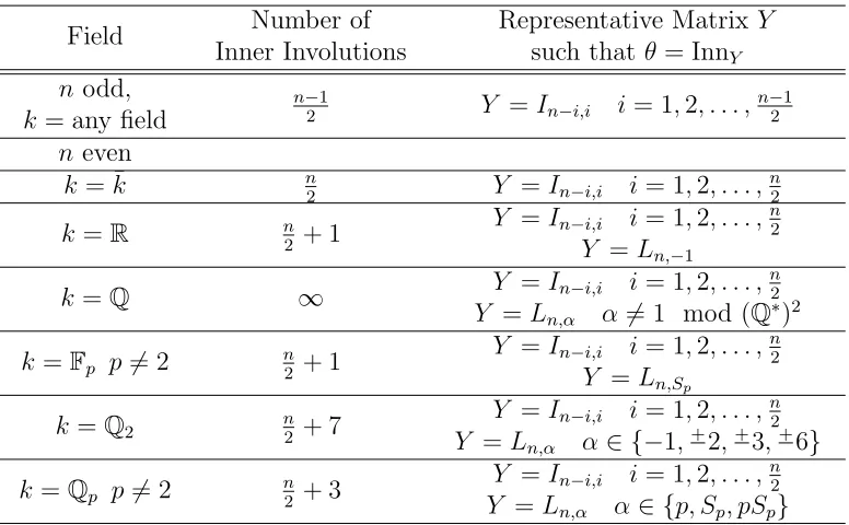
The involutions of G are separated into two groups-the inner involutions and the outer involutions. We will start with outer involutions, specifically θ(X) = (XT)−1. All
whereM comes from a bilinear form. Depending on the fieldk and the size of the matrices we are considering, this could give us a large number of involutions to characterize. For example, if k = Qp with p ∼= 1 mod 4 and n is even, then there are a total of n2 + 9
isomorphism classes of involutions.
Remark 1.4.4. Like SL(2, k), SL(n, k) is ak-split group, meaning that SL(n, k) contains a maximal torus that is also maximal k-split, namely the set of diagonal matrices T. In this case, minimal parabolic k-subgroups are Borel subgroups. Therefore, if we let B be a Borel subgroup containing T, the classification of Bk\Gk/Hk is the exact same as
Pk\Gk/Hk.
We will build posets of standard tori in order to classify the conjugacy classes of θ-stable, maximal k-split tori. We will first need to consider theHk-conjugacy classes of
maximal (θ, k)-split tori. This will tell us the number of tori on the top level of our poset. The results for this are found in Chapter 5. A summary of the results is below.
Theorem 5.2.1 Let θ = Inn∗In−i,i such that i < n/2. Then there exists only one Hk
-conjugacy class of maximal (θ, k)-split tori with representative
A1 ={diag(a1, . . . , ai, a−i 1, . . . , a −1
1 ,1, . . . ,1)|ai ∈k∗}.
Theorem 5.2.2Let θ = Inn∗In−i,i such that i=n/2. Note that n must be even. Then the number of Hk-conjugacy classes of maximal (θ, k)-split tori is at most | k
∗/(k∗)2
±1 |.
Corollary 5.2.3 Let θ = Inn∗In−i,i such that i = n/2. Note that n must be even. Addi-tionally, let k be C,R,Fp withp6= 2, orQp. Then the number of Hk-conjugacy classes of
maximal (θ, k)-split tori equals | k∗/±(k1∗)2 |.
Theorem 5.2.4 Let θ = Innn,x. Not that n must be even and x ∈ k∗/(k∗)2, x 6=
1mod(k∗)2. Then the number of H
k-conjugacy classes of maximal (θ, k)-split tori is at
most | k∗/±(k1∗)2 |.
Theorem 5.2.5Letθ = InnJ2m(A
T)−1for allA ∈G. Then there exists oneH
k-conjugacy
class of maximal (θ, k)-split tori with representative
Chapter 6 gives the results of classifying the (θ, k)-singular roots for each involutionθ of SL(n, k). The set of (θ, k)-singular roots will help in constructing the poset of standard tori that areθ-stable and maximal k-split. A summary of results for this follows.
Theorem 6.1.4 Let G = SL(n, k) and θ = (AT)−1. Then Φ+
θ, the set of positive (θ, k)
-singular roots, is the set of all positive roots if −1 ∈ (k∗)2 and Φ+θ is the empty set if
−16∈(k∗)2.
Theorem 6.1.6 Let G= SL(n, k) and θ(A) = InnJ2m(A
T)−1. Then Φ+
θ =∅.
Theorem 6.1.9 Let G= SL(n,R) and θ= InnMi(A
T)−1. Then Φ+
θ ={αn−i,
roots containing αn−i in their sum }.
Theorem 6.1.13 Let G= SL(n,Fp) and θ = InnMi(A
T)−1. Then Φ+
θ ={αn−i,
roots containing αn−i in their sum }.
Theorem 6.2.4 Let G= SL(n, k) and θ˜= Inn
0 0 0 1
0 0 1 0
0 . .. 0 0
1 0 0 0
. Then Φ+θ = ΦA˜n−i,i.
Theorem 6.2.6 Let G= SL(n, k) and θ = Inn(Ln,−1). Then Φ+θ = Φ( ˜An−i,i).
From there, we will check for Hk-conjugacy andH-conjugacy among the rows of the
poset to help in obtaining representatives of the conjugacy classes. This will get us one step closer to classifying the Weyl group quotientsWGk(Ai)/WHk(Ai) and thus the double
cosets Pk\Gk/Hk. We will use the following result to help in checking for conjugacy.
Theorem 7.2.3 For θ= Inn 0 1 1 0
!
, we have
a+b 0 0 a−b
!
= Inn x −y x y
!
a b b a
!
Chapter 2
Preliminaries
2.1
Preliminaries
Throughout this thesis, we will let k be a field with char(k) 6= 0. G will be a reductive algebraic group defined over k. In particular, we will be interested in the special linear group SL(n, k).
Definition 2.1.1. LetMn(k) denote the set of n×n matrices with entries in k. Then
SL(n, k) ={A∈Mn(k)|det(A) = 1}
is the special linear group.
Let θ be an involution, i.e. θ ∈ Aut(G) and θ2 = Id. When k = ¯k, we denote by Ti
the tori ofG. When k 6= ¯k, we denote by Ai the tori ofGk.
Definition 2.1.2. T ⊂Gis atorusif it is connected, abelian, and consists of semisimple elements.
The set Φ(T) (respectively Φ(A)) is the set of roots of T in G (respectivelyA inG). When T ={diag}, then Φ(T) is the set of all positive roots.
Definition 2.1.3. T is θ-stable if θ(T) =T. Then we have T =T+T−, where
1. T+={t∈T |θ(t) =t}◦
Moreover, T+∩T− is finite.
For the case when n = 2, we have that all maximal tori in G are one-dimensional. Thus, for a θ-stable maximal torus T in G= SL(2, k), T =T+ or T =T−.
We call a torus k-split if the torus is able to be diagonalized over the field k. For k = ¯k, all tori are k-split.
Definition 2.1.4. T a torus is called (θ, k)-split if T isk-split and θ-split.
We are interested in two types of splitting of a torus T. The first type of splitting involves the involution θ and will split the torus T into Tθ+ = {t ∈ T | θ(t) = t}◦ and
Tθ− = {t ∈ T | θ(t) = t−1}◦. The second type of splitting involves the field k and will
divide the torus T into Ts and Ta, the k-split part of T and the k-anisotropic part of
T, respectively. Note that if k = ¯k, then T =Ts. Given a maximal (θ, k)-split torus A,
we can find a maximal torus T containing A in which Tθ− is maximal θ-split and Ts is
maximal k-split.
Figure 2.1: Illustration of k-split and θ-split parts of tori
Ts. The two boxes on the right representTθ−. A torusA that is (θ, k)-split is represented
by the upper right box.
It is interesting to look at howHk acts on all of these different tori. There are several
questions to consider.
1. Hk-conjugacy classes of maximal (θ, k)-split tori.
2. Hk-conjugacy classes of k-split tori.
3. Hk-conjugacy classes of θ-split tori.
Note that if k = ¯k, then theH-conjugacy classes andHk-conjugacy classes are
equiv-alent and all tori arek-split. Our interest lies in the first two questions.
2.2
Generalized Symmetric Spaces
We will now cover some basics of symmetric spaces. We will let V =Rn be a Euclidean
vector space. GL(V) is the space of invertible matrices and GL(V)'GL(n,R). We define a symmetric bilinear form B(x, y) =xTM y where M is an n×n matrix andM =MT.
If M = Id, then B(x, y) = xTy is called the dot product. By one of the conditions of
the bilinear form, we have that B(x, x) > 0 if x 6= 0. We denote by A0 the adjoint of A∈GL(V) with respect to B. Then
B(A(x), y) =B(x, A0(y))∀x, y ∈V
Remark 2.2.1. IfM = Id, then A0 =AT. This can be seen as follows.
B(A(x), y) =B(x, A0(y)) (A(x))TM y =xTATM y =xTM A0y
⇒ATM =M A0 Thus, ifM = Id, then AT =A0.
Let θ(A) = (A0)−1, θ : GL(V) → GL(V) and θ2 = Id. Then θ is an involution. Let
Definition 2.2.2. Let the set Q = {Aθ(A)−1 | A ∈ GL(V)} = {AA0 | A ∈ GL(V)}.
Then Q is a symmetric space.
If M = Id, thenQ={AAT}
({symmetric matrices}.
Definition 2.2.3. Let ˜Q={A∈ GL(V) |θ(A) =A−1}. Then ˜Q is called the extended
symmetric space.
Lemma 2.2.4. Let Q be a symmetric space and Q˜ the extended symmetric space, as defined above. Then Q⊂Q˜.
Proof. LetAA0 ∈Q. Then
θ(AA0) = (A0)−1((A0)0)−1 = (A0)−1(A−1) = (AA0)−1
ThusAA0 ∈Q˜ and Q⊂Q.˜
A torus A is defined to be a subgroup consisting of commuting semisimple elements. As stated previously, we call a torus A ⊂ G θ-split if θ(a) = a−1 for all a ∈ A. In fact,
all maximal θ-split tori are conjugate under the fixed point group H =Gθ.
Definition 2.2.5. LetG be a real group. Then θ ∈Aut(G) is a Cartan involution if 1. θ2 = id
2. H =Gθ ={x∈G|θ(x) = x}is a (maximal) compact subgroup.
Remark 2.2.6. In this case, compact implies maximal compact, so compact is sufficient.
Any reductive real Lie group has a unique (up to conjugation) Cartan involution. For our cases, in SL(n, k), the Cartan involution is θ= (AT)−1.
In the study of symmetric spaces, the two most important questions are
1. What is the action of the fixed point group Hk onGk/Hk? What kind of orbits do
we get?
2. What is the action of the parabolic k-subgroup on Gk/Hk?
Definition 2.2.7. A subgroup B ⊂G is called a Borel subgroup if 1. B is a maximal solvable subgroup.
2. B is connected.
Example 2.2.8. Let G= GL(n, k). ThenB is the set of upper triangular matrices.
ForH ⊂GwithH solvable, we have thatH can be triangularized simultaneously. In other words, there existsx∈G such that xHx−1 ⊂ {upper triangular matrices}.
Definition 2.2.9. A closed subgroup P of G is a parabolic subgroup if the quotient variety G/P is complete.
A closed subgroup of G is parabolic if and only if it contains a Borel subgroup B. Moreover, parabolic subgroups are connected and self-normalizing: NG(P) =P.
Example 2.2.10. LetG= GL(2,R). Then we have G⊃H = O(2,R) is not a connected
subgroup and thus not parabolic. If we take the connected component of H, H◦ = SO(2,R), then we have a parabolic subgroup of G.
Example 2.2.11. We have stated that forG= GL(n, k),Bis the group of upper triangular matrices. P the group of matrices with blocks on the diagonal and zeros beneath the blocks. The following matrix is an example of a matrix in the parabolic subgroup but not in the Borel subgroup.
∗ ∗ ∗ ∗ ∗ ∗ ∗ ∗ 0 ∗ ∗ ∗ 0 0 ∗ ∗
For the case where k = ¯k, we instead look at the action of the Borel subgroups on G/H, sinceB =P in the algebraically closed case.
We have that A⊂ B ⊂ P ⊂G, where G is an algebraic group defined over the field k, P is a minimal parabolic k-subgroup of G, B is the Borel contained in P and A is a maximal k-split torus.
We will define the centralizer of A in Gin the following way:
We will define the normalizer of A inG in the following way:
NG(A) = {g ∈G|Ag =gA}.
We have the following facts about Borels and parabolics:
1. NG(P) = P and NG(B) = B.
2. For B ⊂Ga Borel, then there exists a maximal torus T ⊂B. 3. B determines the positive roots.
4. Let Φ(T) denote the root system of T and let ∆ ⊂ Φ(T) be a basis determined by B. Then there exists a one-to-one correspondence between subsets of ∆ and parabolic subgroups P ⊃B.
5. For B ⊂ G, B a Borel subgroup, then we have the Bruhat decomposition G =
S
w∈W(T)BwB. Also,B\G/B 'W(T).
From the second fact above, it follows that there is a one-to-one correspondence between Borel subgroups containing T and W(T) = NG(T)/ZG(T) =NG(T)/T.
If θ is the Cartan involution and P ⊂G is a minimal parabolicR-subgroup, then we get
|PR\GR/HR|= 1.
Let τ :G→G, g 7→gθ(g)−1. Then Im(τ) =Q'G/H. We have V={g ∈G|τ(g)∈
NG(A)}. ZG(A)×H acts on Vin the following way: (a, h)∗g =agh. Note that agh∈V:
aghθ(agh)−1 =aghθ(h)−1θ(g)−1θ(a)−1 =aghh−1θ(g)−1θ(a)−1
=agθ(a)−1θ(t)−1 Since gθ(g)−1 ∈ N
G(A), by definition of V, we have that τ(agh) ∈ NG(A) and thus
agh∈V.
We will denote by V the set ofZG(A)×H -orbits in V.
Definition 2.2.12. Let w ∈ W(A). We call w a twisted involution if θ(w) = w−1. We
denote by I the set of twisted involutions.
2.3
Algebraically Closed vs. Non-algebraically Closed
There are some important differences between the cases ofk = ¯k and k6= ¯k.
When k = ¯k, all maximal tori are conjugate. When k 6= ¯k, we get two types of tori: those that are diagonalizable over k and those that are not diagonalizable over k.
Example 2.3.1. LetG= SL(2,C) and GR = SL(2,R). We haveT1 and T2 defined in the
following way:
T1 ={
a 0 0 a−1
!
|a∈k∗}
T2 ={
x y −y x
!
|x2+y2 = 1}
T1 is R-split and T2 is R-anisotropic. When we calculate the eigenvalues for T2, we
get x±iy, which is not in R.
If we consider a different field, it is possible that T2 will not be k-anisotropic. For
example, when k = F5, we have that −1 is a square because −1 = 4 = 22. Thus, we
do not get imaginary eigenvalues and we are able to diagonalize T2, making T2 a k-split
torus. When considering Fp, we have that −1 is a square when p ≡ 1 mod 4 and −1 is
not a square when p≡3 mod 4.
When k = ¯k, we have a reductive group G, involution θ, fixed point group H, and a Borel subgroupB that contains a torus T. We will letTθ be the set of θ-stable maximal tori, V = {g | gθ(g)−1 ∈ NG(T)}, and V = {T ×H orbits on V} ' B \G/H. We have
the map ϕ : V → Tθ/H. We are interested in characterizing Tθ/H in order to classify
the double cosets B\G/H.
Lemma 2.3.2. [18] Assume T1, T2 ∈ Tθ with Ti+ maximal, i.e. T
+
i is a maximal torus
of H. Then there exists an h∈H such that hT1h−1 =T2.
Lemma 2.3.3. [18] Assume T1, T2 ∈ Tθ with Ti− maximal, i.e. T −
i is a maximal θ-split
When k 6= ¯k, we have a reductive group Gk, involution θ, fixed point group Hk,
and a minimal parabolic subgroup Pk that contains a torus A. We will let Aθ be the
set of θ-stable maximal k-split tori, V = {g | gθ(g)−1 ∈ N
G(A)}, and V = {ZG(A)×
H orbits on V} 'Pk\Gk/Hk. We have the map ϕ :V → Aθ/Hk. We are interested in
characterizing Aθ/H
k in order to classify the double cosets Pk\Gk/Hk.
We have the following modified lemmas for the non-algebraically closed case. Lemma 2.3.4. [18] AssumeA1, A2 ∈Aθ withA+i maximal, i.e.A
+
i is a maximal torus of
H. Then there exists anh∈H such that hT1h−1 =T2. Thus A1 and A2 areH-conjugate
but not necessarily Hk-conjugate.
Lemma 2.3.5. [18] Assume A1, A2 ∈Aθ with A−i maximal, i.e. A −
i is a maximal (θ, k)
-split torus. Then there exists an x∈(H.ZG(A1))k such that xT1x−1 =T2.
From Lemma 2.3.5, we have that there are usually infinitely many (θ, k)-split tori but in some cases there is only oneHk-conjugacy class of (θ, k)-split tori. If there is only one
Hk-conjugacy class of (θ, k)-split tori, then the lemma for k= ¯k holds fork 6= ¯k.
For algebraically closed G, B ⊂ G a Borel subgroup, θ ∈ Aut(G), θ2 = id, and H =Gθ the fixed point group, we can classify B\G/H in the following ways:
1. H-orbits on G/B 'B={gBg−1 |g ∈G}. ThenB\G/H 'S
i∈IWG(Ti)/WH(Ti)
where {Ti |i∈I} are theH-conjugacy classes of θ-stable maximal tori.
2. B×H-orbits on G.
3. B-orbits on G/H 'Q={xθ(x)−1 |x∈G}
If we consider G defined over k with k 6= ¯k, we have Gk the k-rational points on G,
Pk the minimal parabolic subgroup defined over k, Pk ⊂ Gk, and A a θ-stable maximal
k-split torus with A ⊂ Pk. Then we can classify the double cosets Pk \Gk/Hk in the
following way:
Pk\Gk/Hk '
[
i∈I
WGk(Ai)/WHk(Ai)
with{Ai |i∈I}the set of representatives ofHk-conjugacy classes ofθ-stable maximal
Example 2.3.6. Let G= SL(2,C), θ(g) = (gT)−1, H ={ a b
−b a
!
|a2+b2 = 1}. Then
GR = SL(2,R). We have that Pk = B = {upper triangular matrices} is the minimal
parabolic R-subgroup. Then
B\G/H '[
i∈I
WG(Ti)/WH(Ti)
BR\GR/HR'[
i∈I
WGR(Ai)/WHR(Ai)
The set {Ti |i∈I}={T1, T2} and{Ai |i∈I}={T1}. The set {Ai |i∈I} does not
contain T2 because T2 cannot be diagonalized over R and thus is not R-split. The Weyl group WG(T1) has representatives in HR and since H = T2, the group WH(T2) = {id}.
So we have
B\G/H ' {WH(T1)/WH(T1), WG(T2)}
BR\GR/HR' {id}
We get three orbits in the algebraically closed case and only one orbit in the non-algebraically closed case.
If we consider k =Q in the previous example, we have that
BQ\GQ/HQ '[
i∈I
WGQ(Ai)/WHQ(Ai).
There are infinitely manyHQ-conjugacy classes ofθ-split tori. This can be seen in the following example.
Example 2.3.7. Let G = SL(2,Q), θ(x) = (xT)−1, B = the Borel subgroup of upper
triangular matrices and A the group of diagonal matrices. In this case the computations work out nicer if we let H = Gθ act from the left and define τ(g) = g−1θ(g) and
VQ ={g ∈GQ |τ(g)∈NGQ(A)}. If g =
a b c d
!
∈SL(2,Q), then
g−1θ(g) = b
2+d2 −ab−cd
−ab−cd a2 +c2
!
if and only if ab +cd = 0. So τ(VQ) ⊂ AQ and it coincides with the set consisting
of r 0
0 r−1
!
with r = x2 + y2, (x, y) ∈
Q2 − {(0,0)}. If z =
v u 0 v−1
!
∈ B and
τ(g) = r 0 0 r−1
!
, then
z−1τ(g)θ(z) = rv
−2+u2r−1 −uvr−1
−uvr−1 v2r−1
!
∈AQ
if and only if u = 0. It follows that r 0 0 r−1
!
and s 0
0 s−1
!
are in the same twisted BQ orbit if and only if r−1s∈(Q∗)2. HenceVQ ∼=⊕p≡1(4)
primeZ
/2Zand the set HQ\GQ/BQ is infinite.
2.4
Lie Algebras
The work done throughout this thesis focuses on Lie groups. It is possible to do similar work with Lie algebras with some adjustments. In fact, some of the calculations are easier when dealing with Lie algebras so it can be beneficial to go between the two.
Let g be a Lie algebra. We will denote by t a maximal toral subalgebra and b a Borel subalgebra, i.e. bis a maximal solvable subalgebra. To go between the Lie algebras and the Lie groups, we take the exponential of the Lie algebra. Note that for tori the exponential map Exp is surjective,T = Exp(t), but for most semisimple Lie groups Exp is not surjective.
Since the operation used in the Lie algebra is addition, we will use the additive inverse in place of the multiplicative inverse used in the Lie group. For example, if we let θ be an involution of g, we call tθ-split ifθ(t) = −t for allt ∈t. This change will apply to all definitions and involutions.
Example 2.4.1. Let θ(A) = (AT)−1 be an involution of G. Then for g, θ(A) = −AT.
Thus, we have that h ={X ∈g | −X = XT}. This fixed point group is much easier to
calculate than the fixed point groupH ={X ∈G|A−1 =AT}.
Many of the results from the Lie group hold for the Lie algebra as well. We have that
have similar definitions for t+ and t−.
2.5
P
k\
G
k/H
kThe motivation behind this thesis focuses on classifying the double cosets Pk\Gk/Hk.
We have the following definitions.
Definition 2.5.1. Given a group G and an involutionθ, we define the fixed point group
H as the groupH =Gθ ={g ∈G|θ(g) =g}.
We will let Gk and Hk denote the k-rational points of Gand H, respectively. We let
NG(H) (respectively NGk(Hk)) denote the normalizer of H in G(respectively Hk in Gk)
and ZG(H) (respectivelyZGk(Hk)) denote the centralizer of H inG (respectively Hk in
Gk).
Example 2.5.2. If G= SL(2,C), then GR will be the 2×2 matrices of determinant one with entries in R.
Now that we have established a group G, an involution θ of G, and the fixed point group H =Gθ associated with this involution, we can define a symmetric variety. Definition 2.5.3. A symmetric variety (or symmetric space) is the set Q ={gθ(g)−1 |
g ∈G} 'G/H. A symmetric k-variety is the set Qk ={gθ(g)−1 |g ∈Gk} 'Gk/Hk.
Helminck and Wang gave the following characterization of Pk\Gk/Hk:
Theorem 2.5.4. [22] Pk\Gk/Hk '
S
Ai∈IWGk(Ai)/WHk(Ai), where I is the set of Hk
-conjugacy classes of θ-stable maximal k-split tori and the Ai are representatives of these
Hk-conjugacy classes.
Thus, to classify Pk\Gk/Hk, we first need to classify the Hk-conjugacy classes of
θ-stable maximalk-split tori.
For maximal (θ, k)-split tori, Helminck and Wang gave the following result:
Theorem 2.5.5. [22] Let A1 andA2 be maximal(θ,k)-split tori. LetT ⊃A1 be maximal
k-split. Then there exists a g ∈(H·ZG(T))k such that gA1g
Example 2.5.6. Let G= SL(2, k), k = ¯k, θ(g) = (gT)−1. Then
H =Gθ ={ a b −b a
!
|a2+b2 = 1}=SO(2, k).
Let T1 =
a 0 0 a−1
!
. We have that T1 is θ-split; for t ∈ T1, θ(t) = (tT)−1 = t−1. Thus
T1 = (T1)−θ. Let T2 = H = SO(2). Then for t ∈ T2, we have that θ(t) = t since T2
is the fixed point group. This means that T2 = (T2)+θ. Any θ-stable maximal torus is
H-conjugate to either T1 orT2. Then
B\G/H 'WG(T1)/WH(T1)∪WG(T2)/WH(T2)
and we have the following:
WG(T1) ={id,
0 1
−1 0
!
}=WH(T1)
Chapter 3
Standard Tori
In the process of classifying the Hk-conjugacy classes of θ-stable maximal k-split tori, it
is sufficient to consider only standard tori. We will first consider standardk-split tori and then look at quasi k-split tori and H-quasi k-split tori.
3.1
Standard
k
-split tori
LetG be a connected reductive algebraic group,θ an involution ofG defined overk and H =Gθ, the fixed point group. Given a θ-stable torus A, we will let A+ = A+
θ ={X ∈
A | θ(X) = X} and A− = A−θ = {X ∈ A | θ(X) = X−1}. Let Aθ
k denote the set of
θ-stable maximal k-split tori of G, Aθ denote the set of θ-stable maximal tori of G and
Aθ
0the set ofθ-stable quasik-split tori ofG, which areH-conjugate to aθ-stable maximal
k-split torus.
TheHk-conjugacy classes ofθ-stable maximalk-split tori are determined by the image
and fibers of the map ζ : Aθk/Hk → Aθ/H. The image of ζ consists of the H-conjugacy
classes of θ-stable maximalk-split tori.
To be able to give a characterization of these in terms of conjugacy classes of in-volutions in a Weyl group, we will first show in this section that every conjugacy class contains a standard torus. We will first start with some definitions.
Definition 3.1.1. A quasi k-split torusis a torus that is conjugate under G to ak-split torus, i.e. A is quasi k-split if
with g ∈G and T a k-split torus.
For quasi k-split tori we define singular roots with respect to the involution. Note that k-split tori are also quasi k-split tori, with g = id. IfA is a quasi k-split torus and α∈Φ(A), then we write Gα =ZG(ker(α)◦).
Definition 3.1.2. The roots of Φ(A) can be divided in four subsets, related to the action of θ, as follows.
(a) θ(α)6=±α. Then α is calledcomplex (relative to θ). (b) θ(α) =−α. Then α is calledreal (relative to θ).
(c) θ(α) =α and θ|Gα 6= id. Then α is callednon-compact imaginary (relative toθ).
(d) θ(α) =α and θ|Gα = id. Then α is calledcompact imaginary (relative toθ).
Definition 3.1.3. Ifα is either a real or non-compact imaginary root, then we call it a θ-singular root.
For k-split tori we have to combine the idea of θ-singular with thek-structure of the group itself. Theθ-singular roots can be divided in those which are singular with respect to the k-structure and those which are not. These are defined as follows.
Definition 3.1.4. A real θ-singular root α∈Φ(A) is called (θ, k)-singular(respectively θ-singular anisotropic) if Gα∩H is isotropic (respectively Gα∩H is anisotropic).
Similarly an imaginary θ-singular root is called (θ, k)-singular(respectivelyθ-singular anisotropic) if Gα has a non-trivial (θ, k)-split torus (respectively Gα has no non-trivial
(θ, k)-split tori).
Similar as for quasi k-split tori we have the following result.
Proposition 3.1.5. [19] Let A be a θ-stable maximal k-split torus of G. Then we have the following.
(1) A+ is a maximal k-split torus of H if and only if Φ(A) has no (θ, k)-singular real
roots.
Let Aθ be the set of θ-stable maximal tori ofG.
Definition 3.1.6. For A1, A2 ∈Aθ, the pair (A1, A2) is called standard ifA−1 ⊂A
−
2 and
A+1 ⊃A+2. In this case, we also say that A1 is standard with respect toA2.
The θ-stable maximal tori of Gcan be put into standard position. Since every conju-gacy class contains a standard torus, it suffices to look at the θ-stable, maximal k-split standard tori.
Lemma 3.1.7. Let A1, A2 ∈ A such that A+1 ⊃ A +
2 (respectively A
−
1 ⊂ A
−
2). Then
there exists x ∈ ZH(A+2) (respectively ZH(A−1)) such that (A1, xA2x−1) is standard. In
particular, if A+1 and A+2 (respectively A−1 and A−2) are H-conjugate, so are A1 and A2.
Proof. LetM ZG(A+2). ThenA
−
1 and A
−
2 are θ-split tori of M. LetA⊂M be a maximal
θ-split torus with A ⊃ A−1. Since A−2 is a maximal θ-split torus of M, there exists an x∈(M∩H)◦ such that xAx−1 =A−
2 and hence xA
−
1x−1 ⊂A
−
2.The proof for the second
statement is similar.
Anyθ-stable maximalk-split torus is standard with respect to one containing a max-imal (θ, k)-split torus (respectively a maxmax-imal k-split torus of H).
Lemma 3.1.8. [19] Let A1 be a θ-stable maximal k-split torus. Then there exists a
standard pair (A, S) of θ-stable maximalk-split tori, with A− maximal (θ, k)-split, S+ a
maximal k-split torus of H and A1 is standard with respect to A and S.
Notation 3.1.9. Let A0 ∈ Aθ0 (respectively S0 ∈ Aθ0) be θ-stable maximal k-split tori of
G, such that A−0 (respectively S0+) is a maximal (θ, k)-split torus of G (respectively a maximalk-split torus ofH). We can choose S0 to be standard with respect toA0. In the
following we fix such a standard pair (S0, A0).
It remains to show that any θ-stable maximal k-split torus is H-conjugate with a θ-stable maximalk-split torus standard with respect to A0 and S0.
Proposition 3.1.10. [19] Let(S0, A0)be a standard pair as above and letA1 ∈Aθ0. Then
A1 is H-conjugate with a θ-stable maximal k-split torus, which is standard with respect
to A0 and S0.
A standard pair (A1, A2) of θ-stable maximal tori ofG gives rise to an involution in
Lemma 3.1.11. Let (A1, A2) be a standard pair of θ-stable maximal k-split tori of G.
Then we have the following conditions:
(i) There exists g ∈ZG(A−1A +
2) such that gA1g−1 =A2.
(ii) If n1 =θ(g)−1g and n2 =θ(g)g−1, then n1 ∈NG(A1) and n2 ∈NG(A2).
(iii) Let w1 and w2 be the images of n1 andn2 in W(A1) andW(A2) respectively. Then
w12 = id, w22 = id, and (A1)+w1 = (A2)
+
w2 =A
−
1A +
2, which characterizes w1 and w2.
Proof. SinceA1 andA2 are maximalk-split tori ofZG(A−1A +
2), the first statement is clear.
For (ii) and (iii), consider first n1. Since g ∈ZG(A−1A +
2) andA1 =A−1A + 2(A
+ 1 ∩g
−1A−
2g)
it suffices to look at A+1 ∩g−1A−
2g. So let x ∈ A + 1 ∩g
−1A−
2g and write x = g
−1tg with
t∈A−2. Then n1xn−11 =θ(g
−1t−1g) = θ(x)−1 =x−1. It follows that
Inn(n1)|A−1A +
2 = id, Inn(n1)|A+1 ∩g
−1A−
2g =−id
which implies that n1 ∈NG(A1), w12 = id and (A1)+w1 =A
−
1A + 2.
The assertion for n2 and w2 follows with a similar argument.
Remark 3.1.12. By (iii) of Lemma 3.1.11, w1 and w2 are independent of the choice of
the element g ∈ZG(A−1A +
1) with gA1g−1 =A2.
The above leads to the following definition of standard involutions:
Definition 3.1.13. LetA1,A2,w1 ∈W(A1) andw2 ∈W(A2) be as in Lemma 3.1.11. We
callw1 (respectivelyw2) theA2-standard involution(respectivelyA1-standard involution)
of W(A1) (resp. W(A2)). Moreover we will call an involution w ∈ W(A2) a k-standard
involution, if there exists a θ-stable maximal k-split torus A3 standard with respect to
A2 such that w is the A3-standard involution in W(A2).
In practice, standard involutions are written as the product of Weyl group elements sα’s, as we will see in Chapter 7.
Remark 3.1.14. To show that the H-conjugacy classes in Aθ
0 correspond to conjugacy
classes of the k-standard involutions, we need to prove first a similar result for Aθ/H,
the H-conjugacy classes of θ-stable maximal quasi k-split tori. Namely if A1, A2 ∈ Aθ0
standard with respect to A0 and h∈H such that hA1h−1 =A2, thenA3 =hA0h−1 and
A0 are θ-stable maximal quasi k-split tori with A−3 and A
−
A1-standard involution and the A2-standard involution are conjugate under W(A0) we
will need to show thatA3 andA0 are actually maximal quasik-split tori of ZG(A−2). This
will be shown in the next section, where we have a closer look at theH-conjugacy classes of θ-stable maximal quasi k-split tori.
3.2
Standard Quasi
k
-split tori
In this section we show that, similar as in the case ofk-split tori, everyH-conjugacy class of θ-stable maximal quasi k-split tori contains a standard torus. The conjugacy classes inAθ/H are not only of importance for a characterization of the double cosets P\G/H,
but also for a classification of the subset Aθ
0/H of Aθ/H. The characterization ofAθ/H
is more complicated then that of Aθ
0/H.
Let Gbe a connected reductive algebraic group, θ an involution of G defined overk. Let H = Gθ be the fixed point group. Let Aθ denote the set of θ-stable maximal quasi k-split tori of G. Let A0 denote a θ-stable maximal k-split torus with A−0 a maximal
(θ, k)-split torus of G and T ⊃ A0 a maximal torus of G, such that Tθ− is a maximal
θ-split torus of G. We write V for τ−1(N
G(A0)).
For k-split tori, we had the concept of two tori being standard with respect to one another. When dealing with quasi k-split tori, we must introduce the idea of almost standard.
Definition 3.2.1. For A1, A2 ∈Aθ, the pair (A1, A2) is calledalmost standard if A−1 ⊂
A−2. An almost standard pair (A1, A2) is called standard if A+1 ⊃A +
2. In these cases, we
also say that A1 isalmost standard (respectively standard) with respect to A2.
Only the −1 eigenspace is able to be put in standard position when we have that two tori are almost standard. We only get standard if we take the maximal quasik-split tori inH to be conjugate.
Allθ-stable maximal quasik-split tori ofGwithA−maximal are conjugate underH0.
This conjugacy of theθ-stable maximal quasi k-split tori Awith A− maximal enables us to show that anyθ-stable maximal quasik-split torus is conjugate to one almost standard with respect to A0.
Proposition 3.2.2. Let A1 be a θ-stable maximal quasi k-split torus of G. Then there
exists h∈H0 such that hA−
1h
−1 ⊂A−
Proof. We use induction with respect to dimA−0 −dimA−1. If dimA−0 −dimA−1 = 1, then sinceA−1 is not maximal there existsλ∈Φ(A1) aθ-singular imaginary root. There exists
g ∈ZG((kerλ)0) such that A2 =gA1g−1 isθ-stable and dimA−2 = dimA
−
1 + 1 = dimA
−
0.
But then A−2 is maximal, thus there exists h ∈ H0 such that hA
2h−1 = A0. Since
A−1 ⊂(kerλ)0 ⊂A
2 it follows that hA−1h
−1 ⊂A−
0.
Assume now that dimA−0 −dimA−1 =k > 0. Letλ ∈Φ(A1) be a θ-singular imaginary
root andg ∈ZG((kerλ)0) such thatA2 =gA1g−1 isθ-stable and dimA−2 = dimA
−
1 + 1 =
dimA−0. Since dimA−0 −dimA−2 = k−1 it follows from the induction hypothesis that there exists h∈H0 such that hA−2 ⊂A−0. SinceA−1 ⊂A−2 the result follows.
Lemma 3.2.3. [19] Let A1 be a θ-stable maximal quasi k-split torus almost standard
with respect to A0. There exists an involution w ∈ W(A0) with (A0)−w ⊂ A −
0 and such
that A−1 = ((A0)−w ∩A −
0)0.
The above Lemma enables us to obtain the following result.
Proposition 3.2.4. [19] Let A0 be as above and let A1 ∈Aθ be a θ-stable maximal quasi
k-split torus, almost standard with respect toA0. Then we have the following conditions:
(i) There exists g ∈ZG(A−1) such that gA1g−1 =A0.
(ii) If A1 is standard with respect to A0, then there exists g ∈ ZG(A−1A +
0) such that
gA1g−1 =A0.
Corollary 3.2.5. Any θ-stable maximal quasi k-split torus is H0-conjugate to one
stan-dard with respect to A0.
Proof. Let A1 be a θ-stable maximal quasi k-split torus ofG. From Proposition 3.2.2 it
follows that we may assume that A1 is almost standard with respect to A0. Similar as
in the proof of Lemma 3.2.3 there exist strongly orthogonal θ-singular imaginary roots α1, . . . , αn ∈Φ(A1) (n = dimA−0 −dimA
−
1) and x∈ZG((A1)w+) such that A2 =xA1x−1
is θ-stable and dimA−2 = dimA−1 +n = dimA−0. Here w =sα1· · ·sαn. By Corollary ??
there existsh ∈H0 such thathA
2h−1 =A0. Let A3 =hA1h−1. Since A−1 ⊂ (A1)+w ⊂A −
2
and A+2 ⊂A+1 it follows that A3− =hA−1h−1 ⊂ A−
0 and A + 3 =hA
+ 1h
−1 ⊃ hA+ 2h
−1 =A+ 0.
This proves the result.
toA0. As in Lemma 3.1.11 we can associate an involution with aθ-stable maximal quasi
k-split torus, standard with respect toA0.
Lemma 3.2.6. [19] Let A0 be as above and let A1 ∈ Aθ be a θ-stable maximal quasi
k-split torus, standard with respect to A0 and g ∈ ZG(A−1A +
0) such that gA1g−1 = A0.
Then we have the following conditions:
(i) If n =θ(g)g−1, then n ∈NG(A0).
(ii) Let w be the image of n in W(A0). Then w2 = e and (A0)+w = A
−
1A +
0, which
characterizes w.
This result follows using a similar argument as in Lemma 3.1.11.
Remark 3.2.7. By (ii) of Lemma 3.2.6, w is independent of the choice of the element
g ∈ZG(A−1A +
0) such that gA1g−1 =A0.
This leads to the following definition of standard involutions for the θ-stable maximal quasik-split torus, standard with respect to A0:
Definition 3.2.8. Let A1 ∈ Aθ and w ∈ W(A0) be as in Lemma 3.2.6. We call w the
A1-standard involution of W(A0). Moreover we will call an involution w0 ∈ W(A0) a
standard involution, if there exists a θ-stable maximal quasi k-split torus A1 standard
with respect to A0 such thatw0 is the A1-standard involution in W(A0).
For a θ-stable k-torus A0 of G, write W(A0, H) for NH(A0)/ZH(A0). We have now
the following result.
Proposition 3.2.9. Assume thatA1, A2 ∈Aθ such that they are standard with respect to
A0. Let w1 andw2 be the A1-standard andA2-standard involutions inW(A0)respectively.
If A1 and A2 are conjugate underH, then w1 and w2 are conjugate under W(A0, H).
Proof. Assume h ∈H0 such that hA1h−1 =A2. Then A3 =hA0h−1 isθ-stable with A−3
maximal. It suffices to show that A3 and A0 are conjugate underH0∩ZG(A−1A + 0).
Let α ∈ Φ(A1) with θ(α) = −α and β the corresponding root in Φ(A2). If A−1 does
not contain any real roots, thenA+i (i= 1,2) is maximal and in this case bothw1 andw2
are maximal involutions in Φ1 = {α ∈ Φ(A0) | θ(α) =−α} and hence conjugate under
Since both α and β correspond to roots in Φ(A0), there exists w ∈ W(A0, H0)
such that w(α) = β. Let h1 ∈ H0 be a representative of w and A4 = h1A1h−11. Then
hh1−1A4h1h−1 = hA1h−1 = A2, hh1−1A0h1h−1 = A3 and hh−11 ∈ ZH(β∨). Using
induc-tion it follows that there exists h2 ∈ ZG(A−2A +
0)∩H0 such that h2A3h−21 = A0. Then
g =h2h∈NH(A0) maps w1 to w2.
Remark 3.2.10. The θ-stable maximal quasi k-split tori A1 with A+1 maximal are not
necessarily conjugate under H can be seen as follows. If T is a θ-stable maximal torus with T+ a maximal torus of H, then N
G(T)6= NH(T). This means that T can contain
several H-conjugacy classes of θ-stable maximal quasi k-split tori. These are basically conjugates of the A+0 part of these tori.
A consequence of this is that there is not a unique minimal element in the set of H-conjugacy classes of θ-stable maximal quasi k-split tori. For the minimal element all we can show is the following:
Lemma 3.2.11. [19] Let S be a θ-stable maximal quasi k-split torus with S+ maximal.
There exists a θ-stable maximal torus T of G with T ⊃S and T+ is a maximal torus of
H.
3.3
Standard H-Quasi
k
-split tori
Many of the results for quasi k-split tori are also true for H-quasi k-split tori.
Definition 3.3.1. An H-quasi k-split torus is a torus that is H-conjugate to a k-split torus, i.e. A is H-quasi k-split if
A=hT h−1 with h∈H and T ak-split torus.
When dealing with maximalH-quasi k-split tori, we no longer have to use the defini-tion for almost standard. This is because all maximal H-quasi tori A with A+ maximal
are conjugate. This gives us a unique bottom to the poset of standard tori.
Chapter 4
SL(2
, k
)
4.1
Introduction to
SL(2
, k
)
In order to help us understand what happens in SL(n, k), we will first work on fully understanding SL(2, k). Since SL(n, k) is made up of multiple blocks of SL(2, k), our understanding of the SL(2, k) case will be very beneficial. We have the following theorem to classify the involutions of SL(2, k).
We will let Inn (a b
c d) be conjugation by the matrix (a bc d), i.e.
Inn a b c d
!
(X) = a b c d
!
(X) a b c d
!−1
.
Theorem 4.1.1. [23] The number of isomorphy classes of involutions over G equals the order of k∗/(k∗)2. Furthermore, the involutions of G are of the form θ = Inn (0 1
m0) for
all m ∈ k∗/(k∗)2. Additionally, if m and q are in the same square class, then Inn (0 1
m0)
is isomorphic to the involution Inn 0 1q0
.
For k = C, we have that there is exactly one involution for SL(2, k), which is θ = Inn (0 1
1 0). For k = R, we have that there are two involutions for SL(2, k), namely θ1 =
Inn ( 0 1
−1 0) and θ2 = Inn (0 11 0). For k = Fp, we will have two cases. If −1 ∈ (k∗)2, then
for k =Fp, there is exactly one involution for SL(2, k), which is θ = Inn (0 11 0). If −1 6∈
(k∗)2, then for k =
Fp, we have that there are two involutions for SL(2, k), namely
θ1 = Inn s0 1p0
wheresp is the smallest nonsquare in Fp and θ2 = Inn (0 11 0). Note that if
4.1.2
k
=
C
Let us first consider k =C. Note thatθ(A) = Inn (0 1
1 0) (A)'(AT)
−1. We have that the
maximal (θ, k)-split torus for this involution is T ={diag}= a0 a−01
.
Theorem 4.1.3. Let G = SL(2, k), θ = (AT)−1. If −1 ∈ (k∗)2, then T1 = x0 x−01
and T2 = −b aa b
are the two Hk-conjugacy classes of θ-stable, maximal k-split tori. If
−16∈(k∗)2, then T
1 is the only Hk-conjugacy class of θ-stable, maximal k-split tori.
Proof. Forθ = (AT)−1, the maximum (θ, k)-split torus isT
1 = x0x0−1
.T2 =Hk = −b aa b
is a θ-stable torus, but we need to check to see if T2 is k-split. To check to see if T2 is
diagonalizable, we find its eigenvalues. We get the characteristic equation
(a−λ)2+b2 = 0
a2−2aλ+λ2+b2 = 0 λ2−2aλ+ 1 = 0
λ=a±√a2−1
λ=a±√−b2
λ =a±b√−1 If −1 ∈ (k∗)2 , we have that T
2 is k-split. If −1 6∈ (k∗)2, then we are not able to go
fromT1 toT2 because T2 would not be k-split.
From this theorem, we have that there are two Hk-conjugacy classes of θ -stable,
k-split tori for k=C. The two representatives are T1 and T2.
The process of going from T1 to T2 is called flipping down the poset. When we move
one level down the poset, we are increasing the dimension of the T+ part of the torus
by one and decreasing the dimension of the T− part of the torus by one. In the SL(2, k) case, we are only able to flip a maximum of one time, since there is only one possible root to flip over, namely α1. When flipping from T1 to T2, we are flipping over the α1
4.1.4
k
=
R
If we consider k=R, then we have two involutions because there are two square classes for the real numbers. Our two involutions are θ1 = Inn (−0 11 0) and θ2 = Inn (0 11 0). Note
that θ1 '(AT)−1. From Theorem 4.1.3, we have that there is one Hk-conjugacy class of
θ1 -stable, k-split tori for k =R with representative T1 because −1 is not a square inR. For θ2, we have that there are two Hk-conjugacy classes of θ -stable, k-split tori for
k = R. The two representatives are T = {diag} and H = Gθ2. If we work through the
characteristic equation, we get the following, noting that a2−b2 = 1:
(a−λ)2−b2 = 0 a2−2aλ+λ2−b2 = 0
λ2−2aλ+ 1 = 0 λ=a±√a2−1
λ=a±√b2
λ=a±b
Thus we get eigenvalues a+b and a−b, both contained in R, so H is R-split. For k = R, we see that for θ1, we are not able to flip down the poset and for θ2 we
are able to flip. If we are unable to flip, then we get that Hk is k-anisotropic.
Definition 4.1.5. Hk isk-anisotropic if it does not contain any non-trivial k-split tori.
For θ = Inn (0 1
m0), we have that Hk is k-anisotropic if and only if m 6∈ ¯1. If m ∈ ¯1,
then Hk contains a maximal k-split torus.
4.1.6
k
=
F
pWhen considering SL(2,Fp), we have two cases. If−1 is a square, then SL(2,Fp) is similar
to the case of SL(2,C). If −1 is not a square, then we are in a similar case to SL(2,R). We have that −1 is a square when p = 1 mod 4 and −1 is not a square when p = 3 mod 4.
Example 4.1.7. For SL(2,F5), we have that−1∈(F∗5)2. This gives us only one involution