http://dx.doi.org/10.17576/jsm-2018-4706-31
Multi-Population Mortality Model: A Practical Approach
(Model Kematian Berbilang Populasi: Suatu Pendekatan Praktik)SITI ROHANI MOHD NOR, FADHILAH YUSOF* & ARIFAH BAHAR
ABSTRACT
The growing number of multi-population mortality models in the recent years signifies the mortality improvement in developed countries. In this case, there exists a narrowing gap of sex-differential in life expectancy between populations; hence multi-population mortality models are designed to assimilate the correlation between populations. The present study considers two extensions of the single-population Lee-Carter model, namely the independent model and augmented common factor model. The independent model incorporates the information between male and female separately whereas the augmented common factor model incorporates the information between male and female simultaneously. The methods are demonstrated in two perspectives: First is by applying them to Malaysian mortality data and second is by comparing the significance of the methods to the annuity pricing. The performances of the two methods are then compared in which has been found that the augmented common factor model is more superior in terms of historical fit, forecast performance, and annuity pricing.
Keywords: Augmented; independent; Lee-Carter; mortality; Stochastic model
ABSTRAK
Peningkatan bilangan model kematian berbilang populasi sejak kebelakangan ini menandakan penambahbaikan tahap kematian di negara maju. Dalam kes ini, terdapat jurang kecil perbezaan seks dalam jangka hayat antara populasi, maka model kematian berbilang populasi direka untuk mengasimilasi hubungan antara populasi. Kajian ini mempertimbangkan dua lanjutan model tunggal populasi Lee-Carter, iaitu model bebas dan model faktor umum yang diperkukuhkan. Model bebas menggabungkan maklumat antara lelaki dan perempuan secara berasingan manakala model faktor umum yang diperkukuhkan menggabungkan maklumat antara lelaki dan perempuan secara serentak. Kaedah ini dapat ditunjukkan dalam dua perspektif: Pertama adalah dengan menggunakannya untuk data kematian Malaysia dan kedua adalah dengan membandingkan kepentingan kaedah dengan penentuan harga anuiti. Prestasi kedua-dua kaedah itu kemudiannya dibandingkan dan telah didapati bahawa model faktor umum yang diperkukuhkan adalah lebih tinggi daripada segi kesesuaian sejarah, prestasi ramalan dan penentuan harga anuiti.
Keywords: Bebas; diperkukuhkan; Lee-Carter; kematian; model stokastik
INTRODUCTION
The number of Malaysian population is expected to increase from 29,240 to 42,113 from year 2010 until 2050 (UN 2013). Furthermore, Wolf (2013) mentioned that the average life expectancy for Malaysian population has increased tremendously from the ages of 54 to 73 for male and ages of 56 to 77 for female since 1950. Despite this positive and constant performance, there are demographers who still assume an uncertain increase in the life expectancy, causing the occurrence of negative issues to the individuals and communities (Oeppen & Vaupel 2002; Villegas 2015). The ramifications of uncertain life expectancy are threefold: Pension providers may incur losses due to prolonged payment of insured’s claim (Dowd et al. 2010), individuals may suffer from limited retirement income (Villegas 2015) and government may be inadequate to provide support in terms of healthcare cost (Roy et al. 2012). In other words, the uncertainty surrounding the life expectancy is one of the key drivers in the existence
of longevity risk. Therefore, there is a need for the governments, pensioners, policymakers and researchers to find the best methods to be used in managing the risk and pointing out the importance of stochastic demographic modelling to quantify the population basis risk. Improper modelling leads to the divergent of the forecasting methods and eventually to the underestimation of future costs.
Their results have shown success in the forecasting performance; however, Li and Lee (2005) introduced a multi-population model that produces better forecast performance in contrast to the single-population model. Their idea on multi-population modelling is driven by the existence of the correlation between groups that are closely related to each other: Such mortality improvement in one country affects the mortality improvement in another country, resulting to a correlated fall in the mortality rate. Since then, numerous extensions based on their method have been investigated. A great deal of research has been conducted on the study of multi-population mortality models outside Malaysia, yet only a small number of research has been conducted on the study of coherent mortality model in Malaysia. Shair et al. (2017a, 2017b) are the only authors that have compared coherent mortality model with its independent model in Malaysia. They found that the multi-population mortality model outperformed the single-population mortality model in terms of overall forecast accuracy.
The spurt of the multi-population mortality models signifies a growing need for insurers to have a proper projected life table for actuarial computations. A life table comprising age-specific mortality rates is vital in order to have a proper annuity product pricing. Since the application of coherent mortality model has been limited to Malaysia, this study explores the impact of two multi-population stochastic models (independent model and augmented common factor model) to the annuity pricing in Malaysia. To the best of our knowledge, the implication of multi-population mortality models on annuity pricing has never been studied in Malaysia. Therefore, this study provides substantial contribution to the annuity pricing in Malaysia by projecting the best estimated life table. The remainder of this paper is organised as follows: Next, we have outline an overview of the multi-population mortality models that are used in this study as well as provides brief information about the pricing of annuities; After that, we describes and introduces the mortality data in Malaysia; Subsequently, we reflects and compares the methods used on Malaysian mortality data as well as analyses the impact of mortality model on annuity pricing; and in the final section, we summarises the main conclusion and final remarks.
MATERIALS AND METHODS
INDEPENDENT LEE-CARTER MODEL
The Lee-Carter method is the single stochastic mortality model formulated by Lee and Carter in 1992. It has since been used by researchers to model the mortality levels. The model equation is as follows:
ln(mx,t) = ax + βxkt + εx,t
where mx,t refers to central death rate at age x and year
t. ax describes the overall mortality rate across ages,
whereas βx is the additional age-specific component that represents the speed of mortality rate response to the change of time-varying mortality index kt. εxt is
the error term of Lee-Carter model with mean zero and variance σδ. Mortality index kt was used to forecast the
series. Lee and Carter (1992) modelled the time series kt
with random walk with drift model following Box and Jenkins (1976) procedure for model identification, which can be expressed as:
d is denoted as the drift parameter which measures the average annual change of mortality series. et is an error
term. The outlier analysis was performed on the time series of mortality index kt. Since parameters βx and kt are
unobserved variables, therefore the least square estimates could be found by using the Singular Value Decomposition (SVD) method. The SVD method was applied to the matrix of ln(mx,t) after subtracting ax.
SVD[ln(mx,t – ax] = ρ1Ux,1Vt,1
where ρ1 is an orthogonal matrix, Ux,1 is a non-negative diagonal matrix, and Vt,1 is a transpose of orthogonal
matrix. Li and Hardy (2011) noted that it is possible to extend the Lee-Carter single-population model to multi-population model by using a combination of several Lee-Carter models to the group of populations individually. This could be done as below:
ln(mx,t,i) = ax,i + βx,ikt,i + εx,t,i (1)
The above formula shows almost a similar process and explanation as the model equation, shown at the beginning of this section, with an added term of i that symbolizes the number of populations involved. The parameters of
βx,i and kt,i were estimated from the historical mortality
data, ln(mx,t,i) – ax,i by using the SVD method.
SVD[ln(mx,t,i) – ax,i] = ρr,iUx,r,iVt,r,i,
where R = rank[ln(mx,t,i) – ax,i]. Since there was only one
single principal component incorporated into the model’s design, the maximum rank value of the Lee-Carter model is R = 1.
SVD[ln(mx,t,i) – ax,i] = ρ1,iUx,1,iVt,1,i (2) In order to obtain the estimates of ρ1,i, Ux,1,i and Vt,1,i, the SVD package was employed in R. On the other hand, the time series kt,i was modelled with the ARIMA model
where d is denoted as drift parameter and et is an error term.
Finally, given the estimated values of the three parameters of x,i, x,i and t,i, the predicted value of the historical
mortality was obtained by: mx,t,i = exp(ax,i + x,i t,i)
For multi-population purposes, this method looks easy to be implemented. However, the independent approach signifies the failure of the method in identifying the recent trends and changes in mortality rate between the groups. Moreover, Li and Hardy (2011) found that it is possible to model population groups independently, but with a few shortcomings. Such shortcomings are a large estimate of the population basis risk, in which the model does not include interdependence between individuals and a high possibility of forecast divergence or cross-over.
AUGMENTED COMMON FACTOR MODEL
Li and Lee (2005) introduced the augmented common factor model where the population could share the same single time-varying, kt and the same single age-specific component, βx. The formula for the augmented common factor model is given by:
ln(mx,t,i) = ax,i + βxkt + εx,t,i
where ax,i is an average row of the combination of population log mortality rates ln(mx,t,i) and εx,t,i is the error term. In order to ensure that the independent model does not diverge, Li and Lee (2005) proposed to capture the central tendencies between the two populations through the parameters of the augmented common factor model which are βx and kt, where bx,1 = bx,2 = βx and kt,1 = kt,2 = kt. Employing the similar SVD estimation procedures in (2), βxkt was estimated from the residuals of the matrix
(ln(mx,t,i) –ax,i), where M is the length of the number of population and wi is the weight of the population. Following
Hyndman et al. (2013) and Kjærgaard et al. (2016), the central tendency of the data was captured using geometric mean; = . Parameter kt is further modelled
by using random walk with drift method: kt = kt–1 + d + et
where d is a drift parameter and et is an error term.
However, imposing similar time-varying and age-specific parameters between the populations were inadequate as it completely ignored the differences between the populations and assumed for the same longevity improvement. This eventually could lead us to unrealistic zero basis risk prediction (Li & Hardy 2011). Therefore, another way to overcome this problem was by incorporating
population-specific factor parameters to the augmented common factor model. The model improved is as follows:
ln(mx,t,i) = ax,i + βxkt + bx,ikt,i + εx,t,i (3)
Parameters βxkt and bx,ikt,i have a similar purpose
like the independent Lee-Carter model, yet dissimilar in terms of the group specification. This dissimilarity is the reason it is referred to as the augmented common factor Lee-Carter model. In order to improve the model fit, Li and Lee (2005) added the age-specific parameter bx,ikt,i in
which the parameters could be estimated by applying the SVD method to the residual of the common factor model’s matrix ln(mx,t,i) – ax,i – βxkt. The first order vector of SVD
was taken into account for the parameter estimation. The SVD package was used in R in order to obtain the estimated matrices.
SVD[ln(mx,t,i) – ax,i – βxkt] = ρ1,iUx,1,iVt,1,i
Finally, the history of time series index kt,i was
modelled using the first-order autoregressive model, AR(1) approaches.
kt,i = φ0,i + φ1,ikt–1,i + d +
where φ0,i and φ1,i are constant parameters and ςt,i is the
error term.
LIFE ANNUITY
Nowadays, the topic on ’life annuity’ has become very important in the subject of pension reform due to its ability to ensure long term and periodic fixed income for the retirees golden years. The formal definition of life annuity according to Ahmadi and Gaillardetz (2015) and Bowers et al. (1997) is a stream amount of payment made at the beginning of n periods. The calculation of the present value for future payments is denoted by:
where Y is the total value for future payment; v(j) symbolizes the discount factor at time j; K(x,t) is the random variable for curtate future lifetime at age x; and time t. There are two types of projected life tables that would be used in order to measure the price of annuity. The first one is the projected rates obtained from the models in equations (1-4) and the second one is the projected rates obtained from Malaysian current life table. The projected values obtained were then estimated into the formula given as follows:
where qx,t is denoted as the probability of an individual with
age x and time t would die between time t and t +1. μx,t = mx,t
is the projected mortality rates of the models considered. Based on the obtained value of qx,t,, the survival probability
of an individual at time t and age x is: px,t = 1 – qx,t
The price of annuity could be formulised as below:
(4)
where M symbolises the projected rates by the two stochastic mortality models used,
k px,t = px+j, t + j, k = 1,2,3, and 0 px,t = 1
The annuity prices using the projected current life tables T could be expressed using the following equation:
(5)
In order to measure the annuity prices in (4) and (5), the current price of zero coupon bond must first be estimated which pays premium RM1 at maturity j:
v(j) = P(0, j)
Ahmadi and Gaillardetz (2015) used the cubic smoothing spline approaches to predict the government yield curve as the rate of the coupon bond is only available
at specific amount of maturities, j. Therefore, their method was used to predict the Malaysia Security Government (MSG) 2011 yield curve that was obtained from Bank Negara Malaysia. After the price of zero coupon bond was computed, the price between and was quantified and compared.
DATA DESCRIPTION
The Malaysian mortality data was collected from the Department of Statistics Malaysia (DOSM). The dataset comprises the number of deaths and the number of exposures for male and female in Malaysia since the beginning of 1980 until 2015. There are a total of 17 age groups for both male and female genders with five-year age span ranging from ages 0 to 80. The formula of the mortality rate is as follows:
where Dx,t,i is the number of deaths; Ex,t,i is the number of
exposures; x = 1,2,3,…, N is the number of age groups; t = 1,2,3,…, T is the number of years; and i = 1,2,…, M is the number of populations.
In this study, the multi-population mortality models are applied to two sets of population in Malaysia, which are male population and female population. The male and female dataset was estimated simultaneously to the Augmented Common Factor model and separately to the Independent model. The data was first transformed into a logarithm of mortality rates ln(mx,t) in order to minimize the existence of any possible high variances occurring among the oldest populations.
Figure 1 describes the log mortality rate for both male and female genders. According to the figure, both genders share the same pattern, in which their mortality increases
FIGURE 1. The rainbow age-specific log death rates plots for males (right) and females (left) for
in all age groups. Moreover, the figure demonstrates the improvement of mortality rate in Malaysia as the time period increases. The only obvious significant difference that can be observe between male and female genders is the existence of volatile accident humps in the male mortality rates with ages ranging between 18 and 40, while accident hump for female mortality rates are much less pronounced at that specified range. For the detailed descriptions of mortality trend and pattern for both genders, the plot of the log mortality rates in the time series dimension is illustrated in Figure 2. The white and black circles represent the male and female, respectively. Generally, only a few age groups were selected to be summarised in Figure 2, which were in the age population of 0 to 25 and 60 to 80. Individuals with ages of 30 to 55 were not plotted since they show almost similar pattern with people of ages 60 to 65.
Figure 2 depicts the crude mortality rates in Malaysia for some selected ages from the year 1980 to 2010. The plot in Figure 2 is in line with the plot in Figure 1 where the mortality rates for all ages decrease as the period increases. At the young adult age (15-25), the male mortality rates show non-linear pattern compared to the female mortality rates. According to Shair et al. (2017a, 2017b), this significant difference might be coming from the 73% of road accidents involving male teenagers. In addition, the plot portrays the data suggesting that women tend to live longer than man. Gjonça et al. (1999) mentioned that this gap is influenced by factors such as behavioural factor and social roles. However, at the ages of 0, 5, 75 and 80, the male and female mortality rates tend to cross with each other. In addition, there exists an obvious jump appearing at the same interval year of 1995 to 2000 for all ages and sexes. Gjonça et al. (1999) reported that it is possible for both mortality gaps to narrow provided that the behavioural factor and social roles are reduced. These similarities and the convergence discussed are important information to be incorporated into the mortality model to avoid forecast divergence from happening.
RESULTS AND DISCUSSION
PARAMETERS ESTIMATE
This section assesses the estimated parameters for the independent model and augmented common factor model, respectively. Estimated parameters ax,i and βx,i are reported
in Table 1, whereas estimated time-varying parameters kt,i
are listed in Table 2. According to Table 1, parameters axi
for all methods exhibit the same values and manifest the expected general shape of mortality schedule across ages. The mortality at early age is high and keeps decreasing as the age groups increase. The mortality rate for each method then started to increase again at age of 50. Other than that, parameter βx,i reflects the relative change of mortality rate of each group. Table 1 shows that individuals at young ages are the ones most affected by the changes in the
log mortality rates for which is consistent with the plot descriptions in Figures 1 and 2.
Based on the summary of kt,i in Table 2, almost a
similar downward trend can be observed in the plot of
kt,i for all genders except for male kt,1 in the augmented
common factor model. From year 1980 until 2010, the time series of both genders decrease steadily; however, around
1997 to 2000, the series inherits a sudden spike. Since kt,i
is a predominant step in mortality model, thus an adequate forecasting model needs to be chosen in detail to give a better forecasting result.
MODELS COMPARISON
In this section, the performances of the two different stochastic mortality models in (1) and (3) were evaluated by using in-sample fit and out-sample forecast performances. Following the estimation procedure of SVD method, 31 period of historical mortality rates were applied to the models considered. The results obtained for the male gender are first illustrated in Figure 3, whereas the plotted figure for the female gender is illustrated in the appendix section labelled as Figure 4. Figures 3 and 4 compare the observed and fitted age-specific mortality rates for models (1-2), for ages of 0 to 80. The black, blue, and red circles represent, respectively, the observed values, independent values, and augmented common factor model values. From Figure 3, it is found that the performances of the two methods are almost identical for several age groups that visualise the downward linear pattern with a slight amount of mortality jumps. However, from the ages of 15 to 40, the augmented common factor model gives the best fitted values compared to the other three mortality models as it could capture the volatile period pattern that had occurred. Upon attaining ages 70 and above, the two methods have almost similar values and the fitted mortality rates are not close to the observed values at higher ages. The figures showing female mortality rates are not as volatile as male, thus the two methods give approximately the same fitted rates. Roughly, the augmented common factor model (3) outperformed model (1) when analysed to all age groups. The goodness-of-fit for each method is further analysed in the next sub-section.
Table 4 is also presented to provide a detailed explanation results shown in Table 3 for ages 0 to 80. Table 4 represents error measurement for male and female genders. Based on Table 4, for male gender, the augmented common factor model is more dominant
within the young age range (accident hump) compared to other models, whereas for female gender, the augmented common factor model is dominant at both young and old ages of the populations. The independent model displays the poorest performance in terms of age-specific fit and
FIGURE 2. The crude mortality rates in Malaysia for some selected ages from 1980 to 2010
TABLE 1. Fitted values ax,i and βx,i(1980-2010)
Independent Augmented Common Factor
Age, x ax,1 βx,1 ax,2 βx,2 βx βx,1 βx,2
0 5 10 15 20 25 30 35 40 45 50 55 60 65 70 75 80 85 -5.789 -7.659 -7.539 -6.649 -6.369 -6.337 -6.160 -5.937 -5.597 -5.185 -4.697 -4.237 -3.744 -3.309 -2.844 -2.477 -2.015 -5.789 0.272 0.203 0.121 0.012 0.048 0.024 -0.036 -0.043 -0.002 0.028 0.055 0.059 0.072 0.053 0.073 0.041 0.022 0.272 5.985 -7.947 -7.960 -7.620 -7.408 -7.243 -6.948 -6.622 -6.200 -5.721 -5.209 -4.727 -4.178 -3.665 -3.111 -2.669 -2.133 5.985 0.149 0.125 0.082 0.065 0.073 0.073 0.071 0.061 0.053 0.038 0.042 0.040 0.056 0.038 0.041 0.006 -0.015 0.149 0.191 0.152 0.096 0.046 0.064 0.055 0.033 0.025 0.034 0.035 0.046 0.046 0.062 0.043 0.053 0.020 -0.001 0.191 -0.053 0.021 0.041 0.160 0.139 0.154 0.169 0.156 0.088 0.022 -0.001 0.014 0.034 0.014 0.009 0.014 0.018 -0.053 0.023 0.043 0.019 0.127 0.110 0.145 0.209 0.189 0.128 0.059 0.031 0.018 0.032 0.017 -0.003 -0.063 -0.083 0.023
TABLE 2. Fitted values kt,1 (1980-2010)
Independent Augmented Common Factor
Time, t kt,1 kt,2 kt kt,1 kt,2
average fit. This might be due to the characteristics of the model that completely ignore the differences between the populations and assume for the same longevity improvement. The statistics in Table 4 validates the
assumptions in Figures 3 and 4 where the independent
model shows a similar downward pattern for all specific ages. Given the overall performance at the bottom of each table, the augmented common factor model displays better historical fit for all ages, as well as for both male and female genders.
Another perspective to take in comparing the performances of the model was by examining the ex-post forecasts. After the data was fitted to the methods used in this study, the forecast period was set up to five years, which is from 2011 to 2015. The forecast results for each method were then compared to the original age-specific death rates. The outcome produced from the forecast errors are then compiled in Table 5 using two approaches, which are mean absolute forecast error (MAFE) and mean absolute percentage error (MAPE). Based on Table 5, similar conclusion is obtained from the out-of-sample forecast error measurements written in which the augmented common factor model outperformed the other independent model for both genders.
PRICING LIFE ANNUITIES
In this section, the evaluation of the annuity prices for the current 2011 life table and the models in (1) and (2) are compared in Table 6. In order to obtain the results as discussed next, several steps must first be acquired before proceeding to the annuity quantifying method.
As explained before, in order to measure the annuity prices in (4) and (5), the current price of zero coupon bond is one of the initial steps required to be estimated. In order to calculate the bond price, Malaysian government’s bond rate was obtained from the Malaysia Security Government (MSG) yield curve, Bank Negara Malaysia. Cubic smoothing spline approaches was used to predict the MSG yield curve.
Upon attaining the price of zero coupon bond, the annuity prices for both male and female genders at the ages of 55 to 60 was then calculated. The range is chosen as these are the minimum and maximum retirement ages in Malaysia. In order to find the annuity prices, a single age group must be produced given the 50-year projected rates obtained from two stochastic mortality models considered in this study (five age groups). Using Li and Chan (2004) approaches, the five-age ranges were interpolated into a single age group. The 0 to 80 age groups were then extrapolated near to the surviving age limit 100.
TABLE 3. In-sample (mortality rates)
Model ER MSE MAPE
Independent 0.8736 0.00465 1.12
Augmented Common Factor 0.9097 0.00330 1.02
TABLE 4. In-sample evaluation for males and female
Age
Males Females
Independent Augmented Independent Augmented
MSE MAPE MSE MAPE MSE MAPE MSE MAPE
FIGURE 3. Observed and fitted age specific death rates for male
TABLE 5. Out sample (mortality rates)
Male Female
Model MAFE MAPE MAFE MAPE
Independent 0.0077 8.9695 0.0063 6.6962
Augmented Common Factor 0.0077 7.1398 0.0059 6.5726
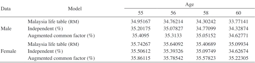
TABLE 6. Annuity prices for period life table and dynamic life table in percentage form (%)
Data Model Age
55 56 58 60
Male Malaysia life table (Independent (%) RM) Augmented common factor (%)
34.95167 35.20175 35.4095
34.76214 35.07827 35.3133
34.30242 34.77099 35.05152
33.77141 34.32874 34.62771
Female Malaysia life table (Independent (%) RM) Augmented common factor (%)
35.74267 35.50612 35.86115
35.64092 35.39326 35.78542
35.40689 35.09749 35.57823
35.09934 34.62674 35.22305
Next, the annuity prices measured from the models in (1-2) was compared with the latest Malaysian mortality table (M9903) released by the Life Insurance Association of Malaysia (LIAM) (Tengku Muda 2017).
Based on Table 6, the annuity prices for both male and female decreased as the ages increased. This is because the younger annuitants needed to pay more for more years of life (Ahmadi & Gaillardetz 2015). In addition, the female annuity prices are much higher as compared to the male annuity prices since the life expectancy of the female gender is much higher than the male gender. The prices for augmented common factor model and Malaysian life table are almost identical with minor differences of 1% to 2% only. The comparisons also showed that the independent model overestimate the Malaysian life table more than the augmented common factor model. In summary, the male and female results indicated that the augmented common factor model has greater expected lifespan compared to other models which eventually leads to greater annuity pricing. As a result, it is better to use the augmented multi-population mortality model in comparison to the independent mortality model as the former captures better longevity risk.
CONCLUSION
This study compared the extensions of the single-population Lee-Carter model to multi-single-population stochastic mortality models in three perspectives which were the in-sample fit, out-of-sample forecast and annuity pricing application. The modelling of the mortality began with the parameter estimation process using the singular value decomposition (SVD) approaches. The historical data was then fitted to the independent model and augmented common factor model. Our numerical analysis showed that the augmented common factor model had better fit and forecast performances as compared to the independent
model. Finally, the impact of stochastic mortality models on the estimation of whole life annuities price was investigated. Among the two methods evaluated, the estimated values of the augmented common factor model were closest to the Malaysian current life table at selected retirement ages for both genders.
ACKNOWLEDGEMENTS
The authors would like to thank the Department of Statistics Malaysia (DOSM) for providing the data as well as to acknowledge Universiti Teknologi Malaysia (UTM) and Kementerian Pelajaran Tinggi Malaysia (KPT) for the financial resources under the Skim Latihan Anak Muda (SLAM) scholarship.
REFERENCES
Ahmadi, S.S. & Gaillardetz, P. 2015. Modeling mortality and pricing life annuities with Lévy processes. Insurance:
Mathematics and Economics 64: 337-350.
Asmuni, N.H. 2015. Essays on annuities and their economic value for retirees. Ph.D. Thesis. Macquarie University Australia (Unpublished).
Bowers, N.L., Gerber, H.U., Hickman, J.C., Jones, D.A. & Nesbitt, C.J. 1997. SAT 472: Actuarial Mathematics. 2nd ed. Schaumburg, Illinois, United States: Society of Actuaries. Box, G.E.P. & Jenkins, G.M. 1976. Time Series Analysis,
Forecasting and Control. San Francisco: Holden Day.
Dowd, K., Blake, D. & Cairns, A.J. 2010. Facing up to uncertain life expectancy: The longevity fan charts. Demography 47(1): 67-78.
Gjonça, A., Tomassini, C. & Vaupel, J.W. 1999. Male-female differences in mortality in the developed world. Rostock: Max Planck Institute for Demographic Research. MPIDR Working Paper WP 1999-009.
Husin, W.Z.W., Zainol, M.S. & Ramli, N.M. 2015. Performance of the Lee-Carter state space model in forecasting mortality.
In Proceedings of the World Congress on Engineering.
Husin, W., Zakiyatussariroh, W., Zainol, M.S. & Ramli, N.M. 2016. Common factor model with multiple trends for forecasting short term mortality. Engineering Letters 24(1). Hyndman, R.J., Booth, H. & Yasmeen, F. 2013. Coherent
mortality forecasting: The product-ratio method with functional time series models. Demography 50(1): 261-283. Ibrahim, R.I. & Siri, Z. 2011. Methods of expanding an abridged
life tables: Comparison between two methods. Sains
Malaysiana 40(12): 1449-53.
Kamaruddin, H.S. 2015. Forecasting mortality rate of malaysia using lee-carter extension of hynman-ullah and booth-maindonald-smith and its statistical comparison analysis. In The 4th Abu Dhabi University Annual International
Conference: Mathematical Science & its Applications.
Kjærgaard, S., Canudas-Romo, V. & Vaupel, J.W. 2016. The importance of the reference populations for coherent mortality forecasting models. In European Population Conference. Lee, R.D. & Carter, L.R. 1992. Modeling and forecasting US
mortality. Journal of the American Statistical Association 87(419): 659-671.
Li, J.S.H. & Hardy, M.R. 2011. Measuring basis risk in longevity hedges. North American Actuarial Journal 15(2): 177-200. Li, N. & Lee, R. 2005. Coherent mortality forecasts for a group
of populations: An extension of the Lee-Carter method.
Demography 42(3): 575-594.
Li, S.H. & Chan, W.S. 2004. Estimation of complete period life Tables for Singaporeans. Journal of Actuarial Practice 11: 129-146.
Ngataman, N., Ibrahim, R.I. & Yusuf, M.M. 2016. Forecasting the mortality rates of Malaysian population using Lee-Carter method. In AIP Conference Proceedings, AIP Publishing 1750 (1): 020009.
Oeppen, J. & Vaupel, J.W. 2002. Broken limits to life expectancy.
Science 296 (5570): 1029-1031.
Roy, A., Punhani, S. & Liyan, S. 2012. How Increasing Longevity
Affects Us All ?: Market, Economic & Social Implications.
London: Global Demographics and Pensions Research.
Shair, S.N., Yusof, A.Y. & Asmuni, N.H. 2017a. Evaluation of the product ratio coherent model in forecasting mortality rates and life expectancy at births by States. In AIP Conference
Proceedings 1842(1): 030010.
Shair, S., Purcal, S. & Parr, N. 2017b. Evaluating extensions to coherent mortality forecasting models. Risks 5(1): 16. Tengku Muda, T.M.M. 2017. Adequacy of employee provident
fund due to longevity Malaysian. The international seminar on Islamic jurisprudence in contemporary society (Islac 2017). Mac 2017. ISBN: 978-967-0899-57-2.
United Nations. 2013. Department of Economic and Social Affairs. Population Division: World Population Prospects: The 2012 Revision.
Villegas Ramirez, A. 2015. Mortality: Modelling, socio-economic differences and basis risk. City University London: Ph.D. Thesis (Unpublished).
Wolf, R. 2013. What’s happening in Malaysia: Getting prepared for retirement ? Allianz International Pensions, (August), pp. 1–11. www.projectm-online.com/research.
Department of Mathematical Sciences Faculty of Science
Universiti Teknologi Malaysia
81310 Johor Bahru, Johor Darul Takzim Malaysia
*Corresponding author; email: [email protected]