Author(s)
Tian, GL; Wang Ng, K; Geng, Z
Citation
Statistica Sinica, 2003, v. 13 n. 1, p. 189-206
Issued Date
2003
URL
http://hdl.handle.net/10722/45356
BAYESIAN COMPUTATION FOR CONTINGENCY TABLES WITH INCOMPLETE CELL-COUNTS
Guo-Liang Tian∗,†, Kai Wang Ng‡ and Zhi Geng∗
∗Peking University, ‡The University of Hong Kong
and †St. Jude Children’s Research Hospital
Abstract: This article studies Bayesian analysis of contingency tables (or multi-nomial data) where the cell counts are not fully observed due to reasons such as nonresponse and misclassification, and derives the posterior distributions of the unknown cell probabilities in terms of various types of generalized Dirichlet tributions. For some special situations such as grouped and nested Dirichlet dis-tributions, the posterior means of the unknown cell probabilities can be obtained in closed form by using inverse Bayes formulae and/or stochastic representation. When closed-form expressions do not exist, we suggest using importance sampling with a feasible proposal density to approximately compute the posterior quantities, and propose a procedure for choosing an effective proposal density. Applications are illustrated by sample surveys with nonresponse, crime survey data, death penalty attitude data, and misclassified multinomial data.
Key words and phrases: Bayesian inference, grouped and nested Dirichlet distribu-tions, incomplete data, inverse Bayes formulae, stochastic representation.
1. Introduction
Statistical procedures for the treatment of missing value problems have re-ceived considerable attention in the past several decades. The advent of the EM algorithm (Dempster, Laird and Rubin (1977)) has virtually revolutionized the practice of frequentist statistics. In a Bayesian framework, the posterior den-sity of the observed data may be difficult to calculate directly. By introducing latent variables or unobserved data, the data augmentation algorithm (Tanner and Wong (1987)) and the Markov chain Monte Carlo (MCMC) or the Gibbs sampler (Gelfand and Smith (1990)) can be used to deal with such problems. No closed-form expressions are obtained for these procedures because they are iterative.
The inverse Bayes formulae (IBF) method of Ng (1995, 1997) can be used to work out closed-form solutions to the incomplete-data problems for some situ-ations. Tan and Tian (2001) obtained some extensive results on the applications of the IBF method to a wide variety of statistical problems, including bivari-ate normal/truncbivari-ated normal/exponential distributions, a genetic linkage model,
misclassified multinomial data, a reliability growth model with missing data, and hierarchical models. With these applications it is argued that the IBF is a useful tool for incomplete data in Bayesian settings. One aim of the paper is to further show that Bayesian computation can be routinely performed by the IBF method when the posterior is a grouped Dirichlet distribution.
This article focuses on Bayesian analysis of contingency tables with incom-plete cell-counts and derives the posteriors of the unknown cell probabilities in terms of various types of generalized Dirichlet distributions. For some special sit-uations such as grouped and nested Dirichlet distributions, the posterior means of the unknown cell probabilities can be obtained in closed form by using the IBF orstochastic representation(SR). When closed-form expressions do not exist, we suggest using importance sampling with a feasible proposal density to approxi-mately compute the posterior quantities, and propose a procedure for choosing an effective proposal density.
Beginning with the formulation of statistical problems, Section 2 provides a closed-form solution by IBF, derives the SRs for the grouped and nested Dirich-let distributions, and suggests importance sampling approximation for the gen-eralized Dirichlet distributions. Section 3 presents applications of the proposed methods to sample surveys with nonresponse, crime survey data, death penalty attitude data, and misclassified multinomial data. In Section 4, we give an il-lustrative example. Section 5 proposes a procedure for choosing an effective proposal density in importance sampling. Finally, a discussion is given and some mathematical proofs are put into the Appendix.
2. Formulation of Problems and Development of Methodology 2.1. Formulation of problems
Consider Bayesian analysis for the contingency tables with incomplete cell-counts. Let Yobs = {y1, . . . , yn; y1∗, . . . , ym∗} denote the observed cell counts and θ be the cell probability vector of interest, where θ ∈ Tn = {(θ1, . . . , θn)> :
θi ≥ 0, i= 1, . . . , n, Pni=1θi = 1}. When there exist some missing cell-counts, the likelihood function L(θ|Yobs) contains two parts:
Qn
i=1θyii — the product of the powers of cell probabilities and Qm
j=1(Pni=1γijθi)y
∗
j — the product of pow-ers of linear combinations of cell probabilities over sets of categories not distin-guished. The Dirichlet distribution D(α1, . . . , αn) is a natural prior distribution with resulting posterior a generalized Dirichlet distribution. Its density is given by f(θ|Yobs) =f(θ|a, b,Γ) =c −1·gD(θ|a, b,Γ) with kernel gD(θ|a, b,Γ) = n Y i=1 θai−1 i ! · m Y j=1 Xn i=1 γijθi bj−1 , θ∈Tn, (2.1)
wherea= (a1, . . . , an)> withai =yi+αi andb= (b1, . . . , bm)> withbj =y∗j + 1 are two known vectors, and Γ = (γij) is an n×m known scale matrix.
Our aim is to compute posterior moments. Denote the simplex by Vn =
{(x1, . . . , xn)> : xi ≥0, i= 1, . . . , n, Pni=1xi ≤1}. It is easy to see thatθ∈Tn is equivalent to θ−n := (θ1, . . . , θn−1)> ∈ Vn−1. The normalizing constant and the posterior moments are given by
c=c(a, b,Γ) = Z Vn−1 gD(θ|a, b,Γ)dθ−n, (2.2) E n Y i=1 θri i = c(a+r, b,Γ) c(a, b,Γ) , where r= (r1, . . . , rn) >. (2.3)
Dickey, Jiang and Kadane (1987) noted that (2.2) has a close relationship with Carlson (1977)’s multiple hypergeometric function and (2.3) can be expressed as ratios of such Carlson’s functions. One method proposed by Kadane (1985) is multinomial expansion of the integrand, and the other is Laplace’s integral method (Tierney and Kadane (1986)) which is approximate. However, both of them are inconvenient for users.
In what follows, we give the closed-form expressions of (2.3), or equivalently (2.2), for two special cases of grouped and nested Dirichlet distributions by IBF and SR. For the generalized Dirichlet distribution, we suggest using importance sampling with a feasible proposal density to approximately compute the posterior moments.
2.2. Inverse Bayes formulae
We briefly introduce the IBF in the context of the general observed/missing data. Tanner and Wong (1987) introduced the concept of data augmentation for calculating the observed posterior densityf(θ|Yobs) when the normalizing constant
is difficulty to compute. The idea is to introduce a latent variable z, which is not observable or missing, such that the complete-data posterior f(θ|Yobs, z) and
the conditional predictive densityf(z|Y0bs, θ) are available. Thenf(θ|Yobs) can be
obtained as an iterative solution of an integral equation. Ng (1995, 1997) noticed a simple analytic solution to that integral equation. Specifically, givenf(θ|Yobs, z)
and f(z|Y0bs, θ), we have f(θ|Yobs) = Z f(z|Y obs, θ) f(θ|Yobs, z) dz −1 = f(θ|Yobs, z0) f(z0|Yobs, θ) Z f(θ|Y obs, z0) f(z0|Yobs, θ) dθ −1 . (2.4)
The first equation of (2.4) is called a pointwise IBF and the last one a functionwise IBF. Note that the functionwise IBF holds for some arbitraryz=z0. Section 3.1
will give the closed-form expression of the posterior mean for grouped Dirichlet distribution by using (2.4).
2.3. Grouped Dirichlet distribution
A generalized Dirichlet distribution (2.1) is called a grouped Dirichlet distri-bution if its density is given by
f(θ|a, b) =c−11· n Y i=1 θai−1 i ! · s X j=1 θj b1−1 Xn j=s+1 θj b2−1 , θ∈Tn, (2.5)
wherea= (a1, . . . , an)> and b= (b1, b2)>. We write θ ∼GDn,2(a, b). Motivated by the SR of a Dirichlet distribution (Fang, Kotz and Ng (1990), p.146), we obtain an SR of θ∼GDn,2(a, b) as follows (see Appendix):
θi=d φiφs, i= 1, . . . , s−1, θs= (1d −Psj=1−1φj)φs,
θi=d φi(1−φs), i=s+ 1, . . . , n−1, θn= (1d −Pj=s+1n−1 φj)(1−φs), (2.6)
where (φ1, . . . , φs−1)>∼D(a1, . . . , as−1;as),φs∼Beta(Psj=1aj+b1−1,Pnj=s+1aj+
b2 −1), (φs+1, . . . , φn−1)> ∼ D(as+1, . . ., an−1;an), and they are independent. Further, (ξ1, . . . , ξn−1)> ∼D(d1, . . . , dn−1;dn) implies that (ξ1, . . . , ξn)> ∼D(d1,
. . . , dn), where ξn = 1−Pnj=1−1ξj. Using the moments of Dirichlet and Beta distributions, one can calculate the high-order moments of a grouped Dirichlet, for instance, E(θi) =E(φi)·E(φs) = ai Ps j=1aj · ( Ps j=1aj)+b1−1 (Pn j=1aj)+b1+b2−2 , i= 1, . . . , s−1, E(θi) =E(φi)·E(1−φs) = ai Pn j=s+1aj · ( Pn j=s+1aj)+b2−1 (Pn j=1aj)+b1+b2−2 , i=s+1, . . . , n−1. (2.7) It is easy to generalize these results to the more general case of a grouped Dirichlet distribution with t partitions, denoted by θ∼GDn,t(a, b). Its density is c−21· n Y i=1 θai−1 i ! · t Y j=1 (θsj−1+1+· · ·+θsj) bj−1, θ∈T n, (2.8) where 0 = s0 < 1 ≤ s1 < · · · < st = n. Similarly, an SR of θ ∼ GDn,t(a, b) with parameter vectors a= (a1, . . . , an)> and b = (b1, . . . , bt)> is given by (see Appendix) θi=d φiφs1, i= 1, . . . , s1−1, θs1 d = (1−Ps1−1 j=1 φj)φs1, θi=d φiφs2, i=s1+ 1, . . . , s2−1, θs2 d = (1−Ps2−1 j=s1+1φj)φs2, .. . ... ... θi d =φiφst, i=st−1+ 1, . . . , st−1, θst d = (1−Pst−1 j=st−1+1φj)φst, (2.9)
where (φ1, . . . , φs1−1) >∼D(a 1, . . . , as1−1;as1), (φs1+1, . . . , φs2−1) >∼D(a s1+1, . . . , as2−1;as2), . . . ,(φst−1+1, . . . , φst−1) >∼D(a st−1+1, . . . , ast−1;ast), (φs1, φs2, . . . , φst) > ∼D(Ps1 k=1ak+b1−1,Pk=ss2 1+1ak +b2−1, . . . , Pst k=st−1+1ak+bt−1), and they
are independent. Then the moments ofθ can be obtained via (2.9).
2.4. Nested Dirichlet distribution
A generalized Dirichlet distribution (2.1) is called a nested Dirichlet distri-bution if its density is given by
c−31· n Y i=1 θai−1 i ! · n−1 Y j=1 Xj k=1 θk bj−1 , θ∈Tn, (2.10)
wherea= (a1, . . . , an)>andb= (b1, . . . , bn−1)>. We writeθ∼NDn,n−1(a, b). As shown in the Appendix, we have the following SR:
θi d = (1−φi−1) n−1 Y j=i φj, φ0 ≡0, i= 1, . . . , n, (2.11)
whereφj ∼Beta(Pjk=1(ak+bk−1), aj+1),j= 1, . . . , n−1, andφ1, . . . , φn−1 are mutually independent. Furthermore, from (2.11), we haveθ1+· · ·+θi
d =Qn−1
j=i φj,
i= 1, . . . , n−1. Then, for example, we obtain
E(θi) =ai·E(θ1+· · ·+θi)/{ i−1 X k=1 (ak+bk−1) +ai}, i= 1, . . . , n, E(θ1+· · ·+θi) = n−1 Y j=i { j X k=1 (ak+bk−1)/[ j X k=1 (ak+bk−1)+aj+1]}, i= 1, . . . , n−1.
2.5. Generalized Dirichlet distribution
Now we calculate the posterior moments (2.3). Our suggestion is first to find a proposal density h(·) defined on Vn−1, and then to estimate c(a, b,Γ) =
R Vn−1{gD(x|a, b,Γ)/h(x)}h(x)dx by ˆ c(a, b,Γ) = 1 M M X k=1 gD(x(k)|a, b,Γ) h(x(k)) , (2.12)
where x(1), . . . , x(M) is an i.i.d. sample of size M from h(·). Feasible choices of h(·) include a Dirichlet distribution D(a1, . . . , an−1;an), a grouped Dirichlet distribution with suitable parameter vectors aandb, and a nested Dirichlet dis-tribution with corresponding parameter vectors aand b. They can be simulated from Beta distributions via (2.6), (2.9) and (2.11).
In Section 5, we propose an effective proposal density in importance sampling for better efficiency. Quasi-Monte Carlo methods can be used in calculating (2.12), readers are referred to Fang, Wang and Bentler (1994).
3. Applications
3.1. Sample surveys with nonresponse
Let n denote the total number of questionnaires sent out. Suppose n1 in-dividuals respond but n2 =n−n1 do not. Of these n1 respondents, there are
y1 individuals whose answers are classified into category A1 and the remaining
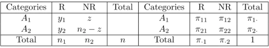
y2 are in A2. Denoting the respondents by R and the nonrespondents by N R, the observed counts and the corresponding cell probabilities may be summarized in Table 1 with π1· as the parameter of interest. Park and Brown (1994) used
the frequentist approach and Albert and Gupta (1985) and Chiu and Sedransk (1986) used the Bayesian approach to study this nonresponse problem. Employ-ing the IBF and the SR of the grouped Dirichlet distribution, we can obtain the exact expression for a Bayesian estimate ofπ1· in dichotomous and polytomous
cases.
Table 1. 2×2 observed counts and corresponding cell probabilities. Categories R NR Total Categories R NR Total
A1 y1 z A1 π11 π12 π1·
A2 y2 n2−z A2 π21 π22 π2·
Total n1 n2 n Total π·1 π·2 1
First we consider the dichotomous case. The observed data is denoted by Yobs = (y1, y2;n2)>, where n2 = n−(y1+y2). A natural latent variable z is
introduced by writing n2 = z+ (n2 −z) and the corresponding cell probabil-ity π·2 = π12+π22. The likelihood function for the complete-data (Yobs, z) is L(Yobs, z|π) ∝π
y1
11π y2
21π12z π22n2−z. If we take D(π|α11, α21, α12, α22) as the prior of
π, then the complete-data posterior distribution isf(π|Yobs, z) = D(π|y1+α11, y2+ α21, z+α12, n2−z+α22). Noting that the conditional predictive density of z givenYobsandπis Binomial(n2, π12/π·2), i.e.,f(z|Yobs, π) =
n2 z π 12 π·2 zπ 22 π·2 n2−z , z= 0,1, . . . , n2, we have, using the pointwise IBF (2.4),
f(π|Yobs) = (n2 X z=0 f(z|Yobs, π) f(π|Yobs, z) )−1 =c−1(α11, α21, α12, α22)π11y1+α11−1π y2+α21−1 21 π12α12−1π22α22−1πn·22,
wherec(α11, α21, α12, α22) =Pnz=02
n2
z
B(y1+α11, y2+α21, z+α12, n2−z+α22). Gunel (1984, p.742) showed that B(a1, a2, a3, a4) = B(a1, a2)B(a3, a4)B(a1 +
a2, a3+a4) for ai >0 (i= 1, . . . ,4), and Pns=0
n
s
B(s+a, n−s+b) =B(a, b). By these identities, we obtainc(α11, α21, α12, α22) =B(y1+α11, y2+α21)B(n1+
α·1, n2+α·2)B(α12, α22). The Bayesian estimate ofπ11isc(α11+ 1, α21, α12, α22) overc(α11, α21, α12, α22), i.e., ˆπ11= (y1+α11)/(n+α··), whereα··=α11+α21+
α12+α22. Similarly, ˆπ12 = (n2 +α·2)α12/{(n+α··)α·2}. Therefore, the Bayes estimator ofπ1·=π11+π12 is (y1+α1·+n2α12/α·2)/(n+α··).
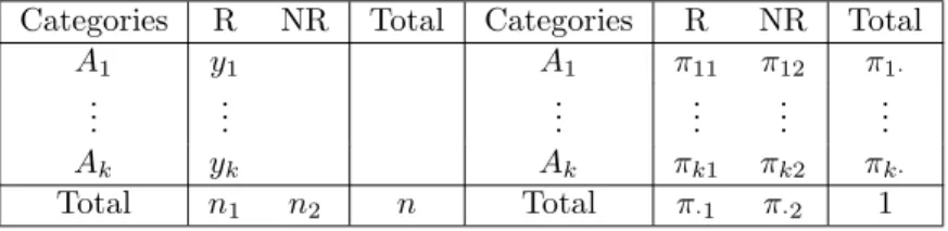
The generalization of the above IBF analysis to the polytomous case is straightforward. Here we apply the SR of a grouped Dirichlet distribution as an alternative approach. The corresponding observed frequencies and cell prob-abilities are displayed in Table 2 with π1·, . . . , πk· as the parameters of interest.
The likelihood function for the observed data is proportional to (Qk
i=1πi1yi)·π·n22, and the prior of π can be taken as D(α). After introducing the reparametriza-tion θ= (θ1, . . . , θk, θk+1, . . . , θ2k)> withθi=πi1 and θk+i =πi2 fori= 1, . . . , k, we know that the observed posterior of θ is proportional to (Q2k
i=1θyii+αi−1)· (Pk
j=1θj)0(P2kj=k+1θj)n2, where yi = 0 for i = k + 1, . . . ,2k. This means that θ ∼ GD2k,2(y +α, b), where y = (y1, . . . , y2k)>, α = (α1, . . . , α2k)> and
b = (1, n2+ 1)>. By (2.7), it is easy to see that the Bayes estimator of π1· is
ˆ
π1·=E(θ1+θk+1) = (y1+α1+αk+1+αk+1n2+α···k+1+α2k)/(n+α·) withα·=
P2k
i=1αi, which coincides with Eq. (2.16) in Basu and Pereira ((1982), p.351).
Table 2. k×2 observed counts and corresponding cell probabilities. Categories R NR Total Categories R NR Total
A1 y1 A1 π11 π12 π1·
..
. ... ... ... ... ...
Ak yk Ak πk1 πk2 πk·
Total n1 n2 n Total π·1 π·2 1
3.2. Crime survey data
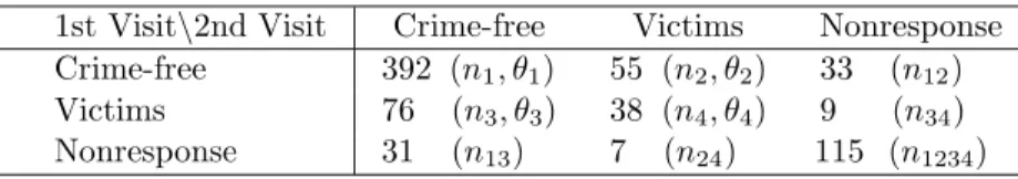
Consider the data set in Table 3 obtained via the National Crime Survey conducted by the U.S. Bureau of the Census (Kadane (1985)). Households are interviewed to see if they had been victimized by crime in the preceding six-month period. The occupants of the same housing unit were reinterviewed again six months later to determine if they had been victimized in the intervening months, whether these were the same people or not. Discarding 115 households, which is equivalent to the assumption ofmissing at random (MAR) or ignorable missing mechanism (Little and Rubin (1987)), Schafer ((1997), p.45, p.271) analyzed
this data set by the EM algorithm from a frequentist perspective. In a Bayesian framework, this data set was originally analyzed by Kadane (1985). Now we denote the probability that a household is crime-free (victimized) in both periods byθ1(θ4), that it is crime-free (victimized) in period 1 and victimized (crime-free) in period 2 byθ2 (θ3). Naturally, θ·=Pj=14 θj = 1, andθj >0 for j = 1, . . . ,4. One of the goals is to obtain the Bayes estimator ofθj.
Table 3. Victimization results from the national crime survey in Kadane (1985). 1st Visit\2nd Visit Crime-free Victims Nonresponse Crime-free 392 (n1, θ1) 55 (n2, θ2) 33 (n12)
Victims 76 (n3, θ3) 38 (n4, θ4) 9 (n34)
Nonresponse 31 (n13) 7 (n24) 115 (n1234)
NOTE: Notations for the observed frequencies of households and probabili-ties are in parentheses.
3.2.1. Nonignorable missing mechanism
Under the assumption of a nonignorable missing mechanism, we have a total of 15 free-parameter π = (πij), a 4×4 matrix, see Table 4. These {πij} are not identifiable unless there is a prior distribution for π. At present,πij can be decomposed as
πij=θjλij, i, j = 1, . . . ,4, (3.1)
whereλ·j =λ1j+· · ·+λ4j = 1 andθj =π1j+· · ·+π4j forj= 1, . . . ,4. Naturally,
λij denotes the corresponding conditional probability, reflecting the prior infor-mation of nonignorability. For instance, λ11 (λ41) is the conditional probability that a household responds (does not respond) in both interviews given that this household is crime-free in both periods. Therefore, in Table 4, responding set R1¯2represents that a household responds in the 1st interview but does not in the 2nd, and the other responding sets have analogous interpretations. Obviously, A1 (A4) represents the category that a household is crime-free (victimized) in both periods. In this way, we can write λ11 = Pr(R12|A1), λ21 = Pr(R1¯2|A1),
λ31= Pr(R¯12|A1) andλ41= Pr(R¯1¯2|A1). The likelihood function is proportional to 4 Y j=1 πnj 1j ·(π21+π22)n12(π23+π24)n34(π31+π33)n13(π32+π34)n24 X4 j=1 π4j n1234 , (3.2) and the prior density can be taken as f(π) ∝ Q4
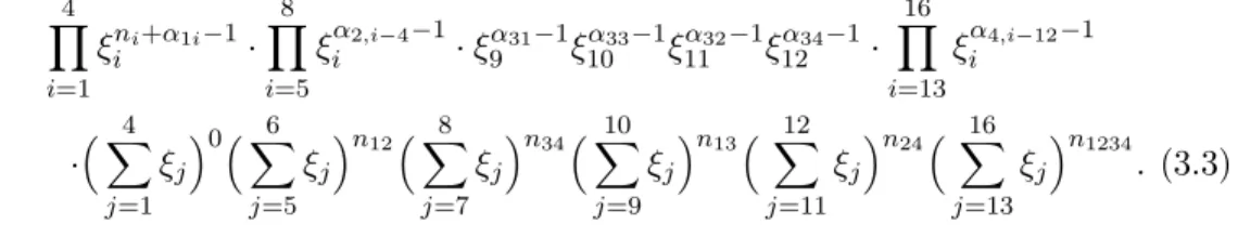
i=1Q4j=1π αij−1 ij . The posterior density is proportional toQ4 j=1π nj+α1j−1 1j Q4i=2Q4j=1π αij−1 ij ·(π21+π22)n12(π23+
π24)n34(π31+π33)n13(π32+π34)n24(P4j=1π4j)n1234, which can be rewritten as, by a straightforward reparametrization, 4 Y i=1 ξni+α1i−1 i · 8 Y i=5 ξα2,i−4−1 i ·ξ α31−1 9 ξ α33−1 10 ξ α32−1 11 ξ α34−1 12 · 16 Y i=13 ξα4,i−12−1 i · 4 X j=1 ξj 0X6 j=5 ξj n12X8 j=7 ξj n34X10 j=9 ξj n13 X12 j=11 ξj n24 X16 j=13 ξj n1234 . (3.3)
Compared with (2.8), we know that (3.3) is a grouped Dirichlet distribution with t = 6 partitions. Then (2.9) can be employed to derive the expectation of ξi,
i= 1, . . . ,16. For instance, E(ξ1) = n1+α11 n+α·· , E(ξ5) = α21(α21+α22+n12) (α21+α22)(n+α··) , E(ξ9) = α31(α31+α33+n13) (α31+α33)(n+α··) , E(ξ13) = α41(α4·+n1234) α4·(n+α··) , (3.4) where n= P4 i=1ni+n12+n34+n13+n24+n1234, α4· =P4j=1α4j, and α·· = P4
i=1P4j=1αij. Therefore, the Bayes estimator for θ1 is given by ˆ
θ1=E(θ1) =E(ξ1) +E(ξ5) +E(ξ9) +E(ξ13). (3.5)
By analogy, the respective posterior means ofθ2, θ3 andθ4 can also be obtained.
Table 4. Parameter structure of nonignorable missing mechanism. Categories R12 R12 R12 R12 R1¯2 R1¯2 R¯12 R¯12 R¯1¯2 Prob. A1 π11 0 0 0 π21 0 π31 0 π41 θ1 A2 0 π12 0 0 π22 0 0 π32 π42 θ2 A3 0 0 π13 0 0 π23 π33 0 π43 θ3 A4 0 0 0 π14 0 π24 0 π34 π44 θ4 Counts n1 n2 n3 n4 n12 n34 n13 n24 n1234 n\1
SOURCE: Kadane (1985). NOTE:R12,R1¯2,R¯12, andR¯1¯2 denote the responding sets.
How do we determine the values of all αij in the prior density? In practice, what we know about is the joint prior of the original parameters {θj}and {λij}, rather than π specified by f(θ, λ1, . . . , λ4), where θ = (θ1, . . . , θ4)> and λj = (λ1j, . . . , λ4j)> for j = 1, . . . ,4, as defined in (3.1). We would like to clarify the relation between f(θ, λ1, . . . , λ4) and f(π). Consider the more general case for (3.1) with i = 1, . . . , k and j = 1, . . . , m. The Jacobian of the transformation (3.1) is Qm
equivalent to saying that θ= (θ1, . . . , θm)> ∼D(α·1, α·2, . . . , α·m), λj = (λ1j, . . . , λkj)>∼D(α1j, α2j, . . . , αkj),
θ, λ1, . . . , λm are mutually independent,
(3.6)
whereθ·= 1 and λ·j = 1 for j= 1, . . . , m. In this way, allαij in priorf(π) can be determined.
3.2.2. An ignorable missing mechanism
An ignorable missing mechanism implies that the elements in each column of the array (λij) are equal. Removing these{λij} from the likelihood function, (3.2) is reduced toQ4
j=1θ nj
j ·(θ1+θ2)n12(θ3+θ4)n34(θ1+θ3)n13(θ2+θ4)n24. Now, D(α1, . . . , α4) is a natural prior for θ = (θ1, . . . , θ4)>. The resulting posterior is a generalized Dirichlet distribution with kernel
gD(θ|a, b,Γ) = 4 Y j=1 θnj+αj−1 j ·(θ1+θ2)n 12(θ 3+θ4)n34(θ1+θ3)n13(θ2+θ4)n24, (3.7) where a = (n1 +α1, . . . , n4 +α4)>, b = (n12+ 1, n34 + 1, n13 + 1, n24 + 1)> and Γ = (γij) with first row (1,0,1,0), and so on. Consequently, the posterior moments for θj, j = 1, . . . ,4, can be obtained by (2.2), (2.3) and (2.12) with proposal density h(θ) =c−h1· 4 Y j=1 θnj+αj−1 j ·(θ1+θ2)n12(θ3+θ4)n34. (3.8)
The proposal density h(θ) is a grouped Dirichlet distribution with normalizing constantch =B(n1+α1, n2+α2)·B(n1+n2+n12+α1+α2, n3+n4+n34+α3+α4)
· B(n3+α3, n4+α4), see (A.2).
The other parameter of interest is the odds ratio (Kadane (1985)), denoted by ψ = θ1θ4/(θ2θ3), one of the ways to measure association in a contingency table. Noting that ψ greater than 1 implies victimization is chronic, the mean and variance of ψ are of interest. In fact, both E(ψ) and E(ψ2) are given by (2.3) with, respectively, r = (1,−1,−1,1) and r = (2,−2,−2,2). Therefore a grouped Dirichlet proposal density h(·) facilitates the computation.
3.3. Death penalty attitude data
Consider Kadane’s data from two sample surveys of juror’s attitudes on a death penalty (Kadane (1983)), in which respondents are classified into four categories: A1 — would not decide guilt versus innocence in a fair and impartial
manner;A2— fair and impartial on guilt versus innocence and, when sentencing, would always vote for the death penalty regardless of circumstance;A3— fair and impartial on guilt and, when sentencing, would never vote for the death penalty; A4 — fair and impartial on guilt and, when sentencing, would sometimes and sometimes not vote for the death penalty. The frequency data y1 = 68, y3 = 97 and y24 = 674 were obtained by a survey of the Field Research Corporation;
y2 = 15 andy134= 1484 by the Harris Survey Company.
Under the assumption of a nonignorable missing mechanism, the combi-nation data of the two-count sets are exhibited in Table 5 which bears some analogy to Table 4. Especially, for the MAR case, the combined likelihood is (Q4
j=1θ nj
j )(θ2+θ4)n24(θ1+θ3+θ4)n134. The Dirichlet prior D(α1, . . . , α4) is ad-equate for θ= (θ1, . . . , θ4)>, which leads to a posterior of a generalized Dirichlet distribution with kernel gD(θ|a, b,Γ) = (Q4
j=1θ
nj+αj−1
j )θ10(θ1 +θ3)0(θ1 +θ3+
θ4)n134 ·(θ2 +θ4)n24. Accordingly, the posterior moments of θj, j = 1, . . . ,4, can be obtained by (2.2), (2.3) and (2.12) with proposal density h(θ) = c−h1·
(Q4
j=1θ
nj+αj−1
j )θ01(θ1+θ3)0(θ1+θ3+θ4)n134, a nested Dirichlet with normalizing constantch=B(a1, a2)B(a1+a2, a3)B(a1+a2+a3+n134, a4), whereaj =nj+αj forj= 1, . . . ,4, see (A.4).
Table 5. Combination data for death penalty attitudes.
Categories R1 R2 R3 R4 R24 R134 Prob. A1 π11 0 0 0 0 π31 θ1 A2 0 π12 0 0 π22 0 θ2 A3 0 0 π13 0 0 π33 θ3 A4 0 0 0 π14 π24 π34 θ4 Counts 68 (n1) 15 (n2) 97 (n3) 0 (n4) 674 (n24) 1484 (n134) 2338 (n)\1
SOURCE: Kadane (1983). NOTE:R1–R4,R24, andR134 denote the responding sets.
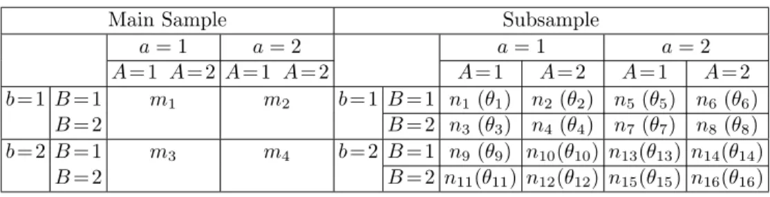
3.4. Misclassified multinomial data
In this section, we demonstrate the potential of our approach for the Bayesian analysis of cell probabilities in categorical data with misclassifications. Geng and Asano (1989) considered a contingency table with binary error-free variables A and B, and denoted the corresponding error-prone variables as aand b, respec-tively. The observed counts of the main sample categorized imprecisely and a subsample categorized both imprecisely and precisely, and the corresponding cell probabilities, are shown in Table 6. The objective is to find the posterior means of cell probabilities of a contingency table categorized by error-free variables, i.e., Pr(A= 1, B = 1) =θ1+θ5+θ9+θ13, Pr(A= 2, B = 1) =θ2+θ6+θ10+θ14, Pr(A= 1, B= 2) =θ3+θ7+θ11+θ15, and Pr(A= 2, B= 2) =θ4+θ8+θ12+θ16.
Table 6. Counts and probabilities for main sample And subsample. Main Sample Subsample
a= 1 a= 2 a= 1 a= 2 A= 1 A= 2 A= 1 A= 2 A= 1 A= 2 A= 1 A= 2 b= 1 B= 1 m1 m2 b= 1 B= 1 n1(θ1) n2(θ2) n5(θ5) n6(θ6) B= 2 B= 2 n3(θ3) n4(θ4) n7(θ7) n8(θ8) b= 2 B= 1 m3 m4 b= 2 B= 1 n9(θ9) n10(θ10) n13(θ13) n14(θ14) B= 2 B= 2 n11(θ11) n12(θ12) n15(θ15) n16(θ16)
Under the assumption of MAR, we take a Dirichlet prior D(α1, . . . , α16), then the posterior of θ = (θ1, . . . , θ16)> is proportional to Q16i=1θaii−1(
P4
j=1θj)m1× (P8
j=5θj)m2(Pj=912 θj)m3(P16j=13θj)m4 with ai = ni +αi for i = 1, . . . ,16, a grouped Dirichlet distribution. Using (2.9), we have
E(θi) = ai a·+m· 1 +P4m1 j=1aj ! , i= 1, . . . ,4, E(θi) = ai a·+m· 1 +P8m2 j=5aj ! , i= 5, . . . ,8, E(θi) = ai a·+m· 1 +P12m3 j=9aj ! , i= 9, . . . ,12, E(θi) = ai a·+m· 1 +P16m4 j=13aj ! , i= 13, . . . ,16,
wherea·=n·+α·=P16i=1(ni+αi) andm·=P4i=1mi.
Geng and Asano also considered the following case. Let A and B be two error-free binary variables. Suppose there is an error-prone variable b for B. Assume that observations in a main sample are categorized byAandb. To obtain information on misclassifications of the error-prone variable b, we observe, from the same population, a random supplemental sample which is categorized by B andb. The observations can be represented as in Table 7. The goal is to find the posterior means of cell probabilities Pr(A= 1, B= 1) =θ1+θ5, Pr(A= 2, B= 1) =θ3+θ7, Pr(A= 1, B= 2) =θ2+θ6, and Pr(A= 2, B= 2) =θ4+θ8.
Under the assumptions of MAR, we take D(α1, . . . , α8) as the prior. Then the posterior for θ= (θ1, . . . , θ8)> is proportional toQ8j=1θ
αj−1
j (θ1+θ2)m12(θ3+
θ4)m34(θ5+θ6)m56(θ7+θ8)m78·(θ1+θ3)n13(θ2+θ4)n24(θ5+θ7)n57(θ6+θ8)n68, a generalized Dirichlet distribution. The meansE(Q8
j=1θ rj
j ) can be calculated by importance sampling (see, (2.2), (2.3), and (2.12)) with proposal densityh(θ) = c−h1·Q8
j=1θ
rj+αj−1
j (θ1+θ2)m12(θ3 +θ4)m34(θ5+θ6)m56(θ7 +θ8)m78, a grouped Dirichlet with normalizing constant ch =B(a1, a2)B(a3, a4)B(a5, a6)B(a7, a8)×
B(a1+a2+m12, a3+a4+m34, a5+a6+m56, a7+a8+m78), whereaj =rj+αj forj= 1, . . . ,8, see (A.3).
Table 7. Observations for main and supplemental samples. Main Sample Supplemental Sample
A= 1 A= 2 A= 1 A= 2 b= 1 B = 1 m12 m34 b= 1 B= 1 (θ1) n13 (θ3) B= 2 B= 2 (θ2) n24 (θ4) b= 2 B = 1 m56 m78 b= 2 B= 1 (θ5) n57 (θ7) B= 2 B= 2 (θ6) n68 (θ8) 4. An Illustrative Example
In this section the crime survey data, Table 3, is used to demonstrate the proposed methods. The goal is to obtain Bayes estimates of θi, i = 1, . . . ,4. We first consider the situation of a nonignorable missing mechanism. Equations (3.4) and (3.5) give the Bayes estimator of θ1. Similarly, we have ˆθ2 =E(θ2) =
E(ξ2)+E(ξ6)+E(ξ11)+E(ξ14), ˆθ3 =E(θ3) =E(ξ3)+E(ξ7)+E(ξ10)+E(ξ15) and ˆ θ4=E(θ4) =E(ξ4) +E(ξ8) +E(ξ12) +E(ξ16), whereE(ξi) = (ni+α1i)/(n+α··), i= 1,2,3,4, E(ξ5) =α21d12, E(ξ6) = α22d12, E(ξ7) = α23d34, E(ξ8) = α24d34, E(ξ9) = α31d13, E(ξ10) = α33d13, E(ξ11) = α32d24, E(ξ12) = α34d24, E(ξ13) = α41d1234, E(ξ14) =α42d1234, E(ξ15) =α43d1234, E(ξ16) =α44d1234, and d12= α21+α22+n12 (α21+α22)(n+α··) , d34= α23+α24+n34 (α23+α24)(n+α··) , d13= α31+α33+n13 (α31+α33)(n+α··) , d24= α32+α34+n24 (α32+α34)(n+α··) , d1234= α4·+n1234 α4·(n+α··) . The corresponding variance and standard deviation (SD) of θi can be obtained by calculating the variance of ξi and the covariance of ξi andξj with (2.9).
We consider two prior distributions. The first is a uniform prior withαij= 1 for all i, j = 1, . . . ,4. From (3.6), this is equivalent to saying θ= (θ1, . . . , θ4)>∼ D(4,4,4,4), λj ∼ D(1,1,1,1), for j = 1, . . . ,4, and θ, λ1, . . . , λ4 are mutually independent. The second prior represents the opinion of experts taken as θ ∼
D(10,5,5,10), λ1 ∼ D(1,3,2,4), λ2 ∼ D(1,0.5,2,1.5), λ3 ∼ D(1.5,2,0.5,1),
λ4 ∼ D(4,2,3,1), and they are independent. Table 8 summarizes results that indicate that the posterior means are slightly sensitive to the choice of the prior.
Table 8. Posterior mean and SD under nonignorable missing mechanism. Priors E(θ1) E(θ2) E(θ3) E(θ4)
Uniform 0.5916 0.1396 0.1668 0.1020 (0.0125) (0.0137) (0.0180) (0.0102) Experts 0.6570 0.1152 0.1362 0.0916
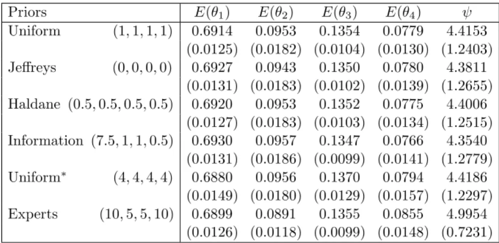
Now we consider the situation of an ignorable missing mechanism. We want to calculate the posterior mean and SD ofθi and the odds ratioψ=θ1θ4/(θ2θ3). The prior for θ = (θ1, . . . , θ4)> is specified by D(α), where α = (α1, . . . , α4)>. Six prior distributions are discussed by Kadane (1985). They are (i) a uniform prior with α = (1,1,1,1)>; (ii) a Haldane prior with α = (0,0,0,0)>; (iii) a Jeffreys prior withα = (0.5,0.5,0.5,0.5)>; (iv) Kadane’s information prior with α= (7.5,1,1,0.5)>; (v) the prior corresponding the uniform prior in Table 8 with
α = (4,4,4,4)>; (vi) the experts prior withα = (10,5,5,10)>. Table 9 displays
outcomes which show that the posterior means are robust to the choice of the prior.
Table 9. Posterior mean and SD under ignorable missing mechanism. Priors E(θ1) E(θ2) E(θ3) E(θ4) ψ Uniform (1,1,1,1) 0.6914 0.0953 0.1354 0.0779 4.4153 (0.0125) (0.0182) (0.0104) (0.0130) (1.2403) Jeffreys (0,0,0,0) 0.6927 0.0943 0.1350 0.0780 4.3811 (0.0131) (0.0183) (0.0102) (0.0139) (1.2655) Haldane (0.5,0.5,0.5,0.5) 0.6920 0.0953 0.1352 0.0775 4.4006 (0.0127) (0.0183) (0.0103) (0.0134) (1.2515) Information (7.5,1,1,0.5) 0.6930 0.0957 0.1347 0.0766 4.3540 (0.0131) (0.0186) (0.0099) (0.0141) (1.2779) Uniform∗ (4,4,4,4) 0.6880 0.0956 0.1370 0.0794 4.4186 (0.0149) (0.0180) (0.0129) (0.0157) (1.2297) Experts (10,5,5,10) 0.6899 0.0891 0.1355 0.0855 4.9954 (0.0126) (0.0118) (0.0099) (0.0148) (0.7231)
5. Choice of Effective Proposal Density
We return to (2.12) and consider the approximation of the normalizing con-stant. In importance sampling, the usual difficulty is finding a suitable proposal density h(·) which mimics the target function gD(·|a, b,Γ). A multivariate split normal/Student proposal density suggested by Geweke (1989) seems infeasible for the present situation since θ belongs to the hyperplane Tn. In Section 2.5, we suggest three feasible choices for h(·). Two questions emerge: (i) what is a natural class of proposal densities? (ii) which member of the class is the most effective? In what follows, we partially answer these questions.
Clearly, the functionwise IBF (2.4) provides a natural class of proposal den-sities: the complete-data posterior densities {f(θ|Yobs, z0) : z0 ∈ S(z|Yobs)}, where
S(z|Yobs)denotes the conditional support ofz. However, the efficiency for
approxi-mating the normalizing constantc=R
f(θ|Yobs, z0)/f(z0|Yobs, θ)dθ by importance
sampling depends on how well the proposal density f(θ|Yobs, z0) mimics the
the observed posterior f(θ|Yobs). The EM algorithm shows thatf(θ|Yobs, z0) and f(θ|Yobs) share the same mode ˆθobs, where
z0=E(z|Yobs,θˆobs). (5.1)
Thus, there is substantial amount of overlapping area under the proposal density and the target function. Thenf(θ|Yobs, z0), withz0 given by (5.1), is heuristically
an effective proposal density.
Now we use the crime survey data under the assumption of an ignorable missing mechanism to illustrate our idea. Return to Section 3.2.2 and denote the observed data byYobs={n1, n2, n3, n4, n12, n34, n13, n24}. Note that the observed
posterior density f(θ|Yobs) is proportional to gD(θ|a, b,Γ) given in (3.7). We
introduce a latent vector z= (z13, z24)> such that the complete-data posterior is
f(θ|Yobs, z)∝θ n1+z13+α1−1 1 θ n2+z24+α2−1 2 θ n3+n13−z13+α3−1 3 θ n4+n24−z24+α4−1 4 ·(θ1+θ2)n12(θ3+θ4)n34, (5.2) and the conditional predictive density is given by
f(z|Yobs, θ) = Binomial z13 n13, θ1 θ1+θ3 ·Binomial z24 n24, θ2 θ2+θ4 . (5.3)
Based on (5.2) and (5.3), the EM algorithm can be used to find the posterior mode ˆ
θobs and z0 = E(z|Yobs,θˆobs). Then an effective proposal density is f(θ|Yobs, z0).
Comparing f(θ|Yobs, z0) with (3.8), we know that both of them belong to the
same class of proposal densities and they are very closed. Therefore the proposal density (3.8) is feasible but not the best andf(θ|Yobs, z0) is the best at the expense
of running an EM algorithm.
6. Discussion
In this paper, we study the Bayesian computations of the posterior moments of the unknown cell probabilities for the contingency table with incomplete cell-counts. For some special cases where the posterior is a grouped or a nested Dirichlet distribution, the posterior means of the unknown cell probabilities can be obtained in closed form by using inverse Bayes formulae and stochastic rep-resentation.
When closed-form expressions do not exist, we suggest using importance sampling to approximately compute the posterior quantities. Three feasible pro-posal densities are suggested and propose a procedure for choosing an effective proposal density. We have noted that Var(θ|Yobs, z0) ≤ Var (θ|Yobs) contradicts
with the common request in importance sampling that the tails of proposal den-sity do not decay more quickly than the tails of the target function (Geweke
(1989)). Our procedure is not perfect, but it provides a universal way to find an effective proposal density for the situation where Var(θ|Yobs, z0) is not much less
than Var (θ|Yobs). Since no methods currently exist for assessing the efficiency of a
proposal density and the accuracy of an importance sampling estimate (Gelman, Carlin, Stern and Rubin (1995), p.307), it is a problem worthy of further study.
Acknowledgements
The research was partially supported by Chinese NSF grants CNSF-19820224 and CNSF-19831010, by a University of Hong Kong CRGC grant, by a U.S. National Cancer Center grant CA21765 and by the American, Lebanese, Syrian Associated Charities (ALSAC). Part of the research was carried out while the first author was visiting the Department of Statistics and Actuarial Science of the University of Hong Kong. We are grateful to an associate editor and two referees for many helpful comments and suggestions on an earlier version of this article.
Appendix
A.1. Derivation of (2.6)
Let θ ∼ GDn,2(a, b) with density given by (2.5). The transformation φi =
θi/Psj=1θj,i= 1, . . . , s−1,φs =Psj=1θj,φi =θi/Pnj=s+1θj,i=s+1, . . . , n−1, has an inverse transformation given by (2.6). Noting that the Jacobian |J| = φs−1
s (1−φs)n−s−1, the joint density f(φ1, . . . , φn−1) is
c−11· s−1 Y i=1 φai−1 i 1− s−1 X j=1 φj as−1 ·φa∗1+b1−2 s (1−φs)a ∗ 2+b2−2· n−1 Y i=s+1 φai−1 i 1− n−1 X j=s+1 φj an−1 , (A.1) where a∗1 = Ps
j=1aj and a∗2 = Pnj=s+1aj. Therefore (φ1, . . . , φs−1)>, φs and (φs+1, . . . , φn−1)>are independent Dirichlet distributions, and (2.6) follows. From (A.1), we obtain c1 =B(a1, . . . , as)·B Xs j=1 aj+b1−1, n X j=s+1 aj+b2−1 ·B(as+1, . . . , an). (A.2) A.2. Derivation of (2.9)
Let θ∼GDn,t(a, b) with density given by (2.8). Making the transformation
φi=θi/(θ1+· · ·+θs1), i= 1, . . . , s1−1, φs1 =θ1+· · ·+θs1, φi=θi/(θs1+1+· · ·+θs2), i=s1+ 1, . . . , s2−1, φs2 =θs1+1+· · ·+θs2, .. . φi=θi/(θst−1+1+· · ·+θst), i=st−1+ 1, . . . , st−1, φst =θst−1+1+· · ·+θst,
the inverse transformation is given by (2.9) and the Jacobian is|J|=Qt−1 j=1φ sj−sj−1−1 sj · (1−Pt−1 k=1φsk) st−st−1−1.Partitionφ= (φ 1, . . . , φn)> into (φ∗1, φs1, φ ∗ 2, φs2, . . . , φ ∗ t, φst) >, whereφ∗ j = (φsj−1+1, . . . , φsj−1),j= 1, . . . , t. We knowf(φ1, . . . , φn−1) = f(θ−n)∗ |J|, which leads to φ∗>j ∼D(asj−1+1, . . . , asj−1;asj), j= 1, . . . , t, (φs1, φs2, . . . , φst) >∼DXs1 k=1 ak+b1−1, s2 X k=s1+1 ak+b2−1, . . . , st X k=st−1+1 ak+bt−1 , and they are independent. Thus (2.9) follows. Similar to (A.2), we obtain the normalizing constant c2= t Y j=1 B(asj−1+1, . . . , asj)·B Xs1 k=1 ak+b1−1, . . . , st X k=st−1+1 ak+bt−1 . A.3. Derivation of (2.11)
Letθ∼NDn,n−1(a, b) with density given by (2.10). Making the transforma-tion φi = Pij=1θj/Pi+1j=1θj, i= 1, . . . , n−2, and φn−1 = Pnj=1−1θj, the inverse transformation is given by (2.11) and the Jacobian is |J| = Qn−1
j=1 φ j−1
j . Hence, the joint densityf(φ1, . . . , φn−1) =c−31·Qnj=1−1φ
dj−1
j (1−φj)aj+1−1, which indicates thatφj ∼Beta(dj, aj+1) forj= 1, . . . , n−1, andφ1, . . . , φn−1 are independent, wheredj =Pjk=1(ak+bk−1). Thus (2.11) follows. Similarly,
c3= n−1 Y j=1 B j X k=1 (ak+bk−1), aj+1 . References
Albert, J. H. and Gupta, A. K. (1985). Bayesian methods for binomial data with applications to a nonresponse problem. J. Amer. Statist. Assoc. 80, 167-174.
Basu, D. and Pereira, C. A. de B. (1982). On the Bayesian analysis of categorical data: the problem of nonresponse. J. Statist. Plann. Inference6, 345-362.
Carlson, B. C. (1977). Special Functions of Applied Mathematics. Academic Press, New York. Chiu, H. Y. and Sedransk, J. (1986). A Bayesian procedure for imputing missing values in
sample surveys. J. Amer. Statist. Assoc. 81, 667-676.
Dempster, A. P., Laird, N. M. and Rubin, D. B. (1977). Maximum likelihood from incomplete data via the EM algorithm (with discussion). J. Roy. Statist. Soc. Ser. B39, 1-38.
Dickey, J. M., Jiang, J. M. and Kadane, J. B. (1987). Bayesian methods for censored categorical data. J. Amer. Statist. Assoc. 82, 773-781.
Fang, K. T., Kotz, S. and Ng, K. W. (1990). Symmetric Multivariate and Related Distributions. Chapman and Hall, London.
Fang, K. T., Wang, Y. and Bentler, P. M. (1994). Some applications of number-theoretic methods in statistics. Statist. Sci. 9, 416-428.
Gelfand, A. E. and Smith, A. F. M. (1990). Sampling-based approaches to calculating marginal densities. J. Amer. Statist. Assoc. 85, 398-409.
Gelman, A., Carlin, J. B., Stern, H. S. and Rubin, D. B. (1995). Bayesian Data Analysis. Chapman and Hall, London.
Geng, Z. and Asano, C. (1989). Bayesian estimation methods for categorical data with misclas-sification. Comm. Statist. Theory Methods18, 2935-2954.
Geweke, J. (1989). Bayesian inference in econometric models using Monte Carlo integration.
Econometrica 57, 1317-1339.
Gunel, E. (1984). A Bayesian analysis of the multinomial model for a dichotomous response with nonrespondents. Comm. Statist. Theory Methods13, 737-751.
Kadane, J. B. (1983). Juries hearing death penalty cases: statistical analysis of a legal proce-dure. J. Amer. Statist. Assoc. 78, 544-552.
Kadane, J. B. (1985). Is victimization chronic? a Bayesian analysis of multinomial missing data. J. Econometrics29, 47-67.
Little, R. J. A. and Rubin, D. B. (1987). Statistical Analysis with Missing Data. Wiley, New York.
Ng, K. W. (1995). Explicit formulas for unconditional pdf. Research Report, No. 82 (revised). Department of Statistics, University of Hong Kong.
Ng, K. W. (1997). Inversion of Bayes formula: explicit formulae for unconditional pdf. In
Advance in the Theory and Practice in Statistics(Edited by N. L. Johnson and N. Balakr-ishnan), 571-584. Wiley, New York.
Park, T. and Brown, M. B. (1994). Models for categorical data with nonignorable nonresponse.
J. Amer. Statist. Assoc. 89, 44-52.
Paulino, C. D. M. and Pereira, C. A. de B. (1992). Bayesian analysis of categorical data informatively censored. Comm. Statist. Theory Methods21, 2689-2705.
Schafer, J. L. (1997). Analysis of Incomplete Multivariate data. Chapman and Hall, London. Tanner, M. A. and Wong, W. H. (1987). The calculation of posterior distributions by data
augmentation (with discussion). J. Amer. Statist. Assoc. 82, 528-540.
Tian, G. L. and Tan, M. (2001). Exact statistical solutions using the inverse Bayes formulae. Technical Report #2001-02, Dept. of Biostatistics, St. Jude Children’s Research Hospital, Memphis, TN, USA.
Tierney, L. and Kadane, J. B. (1986). Accurate approximations for posterior moments and marginal densities. J. Amer. Statist. Assoc. 81, 82-86.
Division of Biostatistics, University of Maryland Greenebaum Cancer Center, Baltimore, MD 21201, U.S.A.
E-mail: [email protected]
Department of Statistics and Actuarial Science, the University of Hong Kong, P. R. China. E-mail: [email protected]
Department of Probability and Statistics, Peking University, P. R. China. E-mail: [email protected]