Clemson University
TigerPrints
All Dissertations Dissertations
8-2007
Control Techniques for Robot Manipulator
Systems with Modeling Uncertainties
David Braganza
Clemson University, [email protected]
Follow this and additional works at:https://tigerprints.clemson.edu/all_dissertations
Part of theElectrical and Computer Engineering Commons
This Dissertation is brought to you for free and open access by the Dissertations at TigerPrints. It has been accepted for inclusion in All Dissertations by an authorized administrator of TigerPrints. For more information, please [email protected].
Recommended Citation
Braganza, David, "Control Techniques for Robot Manipulator Systems with Modeling Uncertainties" (2007).All Dissertations. 99.
CONTROL TECHNIQUES FOR ROBOT MANIPULATOR SYSTEMS WITH MODELING UNCERTAINTIES
A Dissertation Presented to the Graduate School of
Clemson University In Partial Fulfillment
of the Requirements for the Degree Doctor of Philosophy
Electrical and Computer Engineering by
David Braganza August 2007 Accepted by:
Dr. Darren M. Dawson, Committee Chair Dr. Ian D. Walker
Dr. John R. Wagner Dr. Timothy C. Burg
ABSTRACT
This dissertation describes the design and implementation of various nonlinear control strategies for robot manipulators whose dynamic or kinematic models are uncertain. Chapter 2 describes the development of an adaptive task-space tracking controller for robot manipulators with uncertainty in the kinematic and dynamic models. The controller is developed based on the unit quaternion representation so that singularities associated with the otherwise commonly used three parameter representations are avoided. Experimental results for a planar application of the Barrett whole arm manipulator (WAM) are provided to illustrate the performance of the developed adaptive controller.
The controller developed in Chapter 2 requires the assumption that the manipu-lator models are linearly parameterizable. However there might be scenarios where the structure of the manipulator dynamic model itself is unknown due to difficulty in modeling. One such example is the continuum or hyper-redundant robot manipulator. These manipulators do not have rigid joints, hence, they are difficult to model and this leads to significant challenges in developing high-performance control algorithms. In Chapter 3, a joint level controller for continuum robots is described which utilizes a neural network feedforward component to compensate for dynamic uncertainties. Experimental results are provided to illustrate that the addition of the neural network feedforward component to the controller provides improved tracking performance.
While Chapter’s 2 and 3 described two different joint controllers for robot ma-nipulators, in Chapter 4 a controller is developed for the specific task of whole arm grasping using a kinematically redundant robot manipulator. The whole arm grasping control problem is broken down into two steps; first, a kinematic level path planner is designed which facilitates the encoding of both the end-effector position as well as the manipulators self-motion positioning information as a desired trajectory for the manipulator joints. Then, the controller described in Chapter 3, which provides
asymptotic tracking of the encoded desired joint trajectory in the presence of dy-namic uncertainties is utilized. Experimental results using the Barrett Whole Arm Manipulator are presented to demonstrate the validity of the approach.
DEDICATION
This dissertation is dedicated to my parents and sisters for the love and support which has made this work possible.
ACKNOWLEDGMENTS
I would like to express my sincere gratitude to Dr. Darren Dawson for his con-stant guidance and encouragement during my dissertation work. I appreciate the opportunity he gave me to work on a number of different projects which has made my research experience at Clemson all the more worthwhile. His professionalism and drive to succeed have truly motivated me to strive for excellence in all my work.
I would also like to thank Dr. Ian Walker for the opportunity to work on the OC-TOR project which enabled me to complete part of the research in this dissertation. I have worked with him quite often in the past couple of years and his passion for robotics and his elegant explanations of complex topics have made learning from him very enjoyable.
This dissertation would not have been possible without the nurturing and support of my parents and sisters, they have kept me from losing sight of my dreams.
My research at CRB has been a great experience and has been helped along by many colleagues. I’d like to thank Michael McIntyre for his patient explanations and help in understanding the paper writing process during the early years of my PhD. Vilas Chitrakaran for always having a solution to robotics or software issues; his professional attitude toward work was also an inspiration. Enver Tatlicioglu for helping me out with all those math problems and for many stimulating discussions.
Finally, my stay at Clemson for almost five years would not have been possible if I didn’t have some wonderful friends to support me, I’d like to thank them all for bearing with me through the tough times.
TABLE OF CONTENTS Page TITLE PAGE . . . i ABSTRACT . . . ii DEDICATION . . . iv ACKNOWLEDGMENTS . . . v
LIST OF TABLES . . . viii
LIST OF FIGURES . . . ix
CHAPTER 1. INTRODUCTION . . . 1
Organization . . . 1
Tracking Control for Robots with Kinematic and Dynamic Uncertainty. . . 1
Neural Network Controller for Continuum Robots . . . 4
Whole Arm Grasping Using Redundant Robot Manipulators . . . 7
2. TRACKING CONTROL FOR ROBOT MANIPU-LATORS WITH KINEMATIC AND DYNAMIC UNCERTAINTY . . . 10
Robot Dynamic and Kinematic Models . . . 10
Problem Statement. . . 14
Tracking Error System Development . . . 17
Stability Analysis . . . 19
Simulation Results . . . 21
Experimental Results . . . 22
3. A NEURAL NETWORK CONTROLLER FOR CONTINUUM ROBOTS . . . 33
Robot Sensing and Actuation . . . 34
Robot Dynamic Model . . . 35
Table of Contents (Continued)
Page
Experimental Results . . . 40
4. WHOLE ARM GRASPING CONTROL FOR REDUNDANT ROBOT MANIPULATORS . . . 50
Manipulator Models . . . 50
High Level Path Planning . . . 52
Low Level Control . . . 58
Experimental Results . . . 61
5. CONCLUSION . . . 71
LIST OF TABLES
Table Page
3.1. Performance measures for the controller with and without the feedforward component calculated for the first 5 seconds of the
experimental trajectory . . . 45 3.2. Performance measures for the controller with and without the
feedforward component calculated for the first 10 seconds of the
experimental trajectory . . . 45 3.3. Performance measures for the controller with and without the
feedforward component calculated for the first 60 seconds of the
LIST OF FIGURES
Figure Page
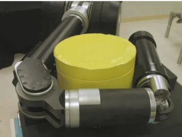
1.1. Whole arm grasping with the Barrett WAM manipulator. . . 8
1.2. Whole arm grasping with the OCTARM continuum manipulator.. . . 8
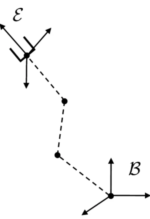
2.1. Representation of coordinate frames for the system. . . 12
2.2. End-effector trajectory tracking error for the simulation. . . 22
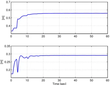
2.3. Kinematic parameter estimates for the simulation. . . 22
2.4. Dynamic parameter estimates for the simulation. . . 23
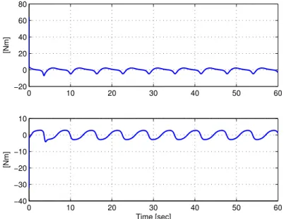
2.5. Control input torque for the simulation. . . 23
2.6. Actual and desired end-effector trajectory for the simulation. . . 24
2.7. Barrett Whole Arm Manipulator. . . 25
2.8. Actual and desired end-effector trajectory (only the last revolution is shown). . . 28
2.9. End-effector position tracking error. . . 29
2.10. Link length estimates. . . 30
2.11. Dynamic parameter estimates. . . 31
2.12. Control input torques. . . 32
3.1. OCTARM VI continuum manipulator grasping a ball in Clemson University’s robotics laboratory. . . 34
3.2. Block diagram showing an overview of the OCTARM VI control system. . . 41
3.3. The OCTARM VI robotic manipulator. . . 42
3.4. Actual and desired length trajectory without neural network component, solid line represents the actual length trajectory, dashed line represents the desired length trajectory. . . 46
List of Figures (Continued)
Figure Page
3.5. Tracking error without neural network component. . . 47
3.6. Control pressure without neural network component. . . 47
3.7. Actual and desired length trajectory with neural network component, solid line represents the actual length trajectory, dashed line represents the desired length trajectory. . . 48
3.8. Tracking error with neural network component. . . 48
3.9. Control pressure with neural network component. . . 49
4.1. Experiment setup showing the Barrett Whole Arm manipulator and object to the grasped. . . 63
4.2. Planar configuration for the three link robot with a circular object. . . 63
4.3. Desired joint angles qd(t) and actual joint anglesq(t). . . 67
4.4. Joint space position tracking errore1(t). . . 68
4.5. Joint space control torquesτ(t). . . 69
4.6. Spatial position Xi ∀i= 1,· · · ,6 (each link and mid-point of the link). . . 70
CHAPTER 1 INTRODUCTION
Organization
This dissertation is organized into four chapters. Chapter 2 presents the develop-ment of an adaptive task-space tracking controller for rigid link robot manipulators with uncertainty in their kinematic and dynamic models. The controller is developed based on the unit quaternion representation to avoid singularities associated with other three parameter representations. Also, the controller does not require the mea-surement of task-space velocities. There might be situations where accurate dynamic modeling of the manipulator is not possible, in these cases it is difficult to implement an adaptive controller as in Chapter 2. With this in mind, in Chapter 3, a joint level neural network tracking controller is presented which can deal with high levels of uncertainty in the robot dynamic model. The neural network based controller is applicable to rigid and flexible link manipulators as well as continuum robot manip-ulators since it does not depend on any specific model of the manipulator. Finally, in Chapter 4, the task of whole arm grasping using a kinematically redundant robot manipulator whose dynamic model is unknown and where the contact forces between the robot and the object are unmeasurable is considered. The whole arm grasping controller is developed by first designing a high level path planner and then using the controller developed in Chapter 3 as the joint level tracking controller. The remainder of this chapter provides an introduction and motivation to study each of the control problems being considered in this dissertation.
Tracking Control for Robots with Kinematic and Dynamic Uncertainty
The control objective in many robot manipulator applications is to command the end-effector motion to achieve a desired response. The control inputs are applied to the manipulator joints, and the desired position and orientation is typically encoded
in terms of a Cartesian coordinate frame attached to the robot end-effector with re-spect to the base frame (i.e., the so-called task-space variables). Hence, a mapping (i.e., the solution of the inverse kinematics) is required to convert the desired task-space trajectory into a form that can be utilized by the joint task-space controller. If there are uncertainties or singularities in the mapping, then this can result in degraded per-formance or unpredictable responses by the manipulator. Several parametrizations exist to describe orientation angles in the task-space to joint-space mapping, including three-parameter representations (e.g., Euler angles, Rodrigues parameters) and the four-parameter representation given by the unit quaternion. Three-parameter repre-sentations always exhibit singular orientations (i.e., the orientation Jacobian matrix in the kinematic equation is singular for some orientations), while the unit quater-nion represents the end-effector orientation without singularities. By utilizing the singularity free unit quaternion, the emphasis of chapter 2 is to develop a tracking controller that compensates for uncertainty throughout the kinematic and dynamic models. Some previous task-space control formulations based on the unit quaternion can be found in [1], [2], [3], [4], [5], and the references therein. A quaternion-based re-solved acceleration controller was presented in [2], and quaternion-based rere-solved rate and resolved acceleration task-space controllers were proposed in [5]. Output feed-back task-space controllers using quaternion feedfeed-back were presented in [3] for the regulation problem and in [1] for the tracking problem. Model-based and adaptive asymptotic full-state feedback controllers and an output feedback controller based on a model-based observer were developed in [4] using the quaternion parametrization.
A common assumption in most of the previous robot controllers (including all of the aforementioned quaternion-based task-space control formulations) is that the robot kinematics and manipulator Jacobian are assumed to be perfectly known. From a review of literature, few controllers have been developed that target uncertainty in the manipulator forward kinematics and Jacobian. For example, in [6], [7], [8], [9], [10], [11], several approximate Jacobian feedback controllers that exploit a static,
best-guess estimate of the manipulator Jacobian to achieve task-space regulation objectives despite parametric uncertainty in the manipulator Jacobian. In [12], a task-space adaptive controller for set point control of robots with uncertainties in the gravity regressor matrix and kinematics was developed. In [13], an adaptive regula-tion controller for robot manipulators with uncertainty in the kinematic and dynamic models was developed. The result in [13] also accounted for actuator saturation since the maximum commanded torque could be a priori determined due to the use of saturated feedback terms in the controller. Recently in [14], an adaptive regulation controller for rigid-link electrically driven robot manipulators with uncertainty in kinematics, manipulator dynamics and actuator dynamics was developed.
All of the aforementioned controllers that account for kinematic uncertainty are based on the three-parameter Euler angle representation. Moreover, all of the previ-ous results only target the set-point regulation problem. The only results which target the more general tracking control problem for manipulators with uncertain kinemat-ics are given in [15], [16], [17]. However, these results are also based on the Euler angle representation and with the exception of [16] they all require the measurement of the task-space velocity. In [16], a filtered derivative of the task-space position is used to generate an approximation of the task-space velocity signal. Hence motivated by previous work, an adaptive tracking controller is developed in chapter 2 for robot manipulators with uncertainty in the kinematic and dynamic models. The controller is developed based on the unit quaternion representation so that singularities asso-ciated with three parameter representations are avoided. In addition, the developed controller does not require the measurement of the task-space velocity. The stability of the controller is proven through a Lyapunov based stability analysis. Experimen-tal results for a planar application of the Barrett whole arm manipulator (WAM) are provided to illustrate the performance of the developed controller.
Neural Network Controller for Continuum Robots
Continuum or hyper-redundant manipulators [18, 19], belong to a special class of robotic manipulators which are designed to exhibit behavior similar to biological trunks [20–23], tentacles [24], or snakes [25]. Unlike traditional rigid link robot ma-nipulators, continuum robot manipulators do not have rigid joints and they have a large number of degrees of freedom, this enables continuum manipulators to have some very useful properties. The continuum manipulators can be compliant, ex-tremely dexterous, flexible, and capable of dynamic adaptive manipulation in highly unstructured environments. These properties of soft continuum robot manipulators make them uniquely suited for a large number of applications, including search and rescue, underwater and space exploration.
The development of high performance model based control algorithms for con-tinuum manipulators is a challenging problem for several reasons; since the manip-ulators must be modeled as continuous curves, the kinematic and dynamic models are difficult to derive, also, the manipulators body is soft and flexible which makes accurate control difficult to achieve. There have been several different approaches which researchers have studied for the control of continuum robot manipulators. For example, Matsuno et al. [26], proposed kinematic control techniques for continuum manipulators and [27–30] described set-point controllers for continuum manipulators. In [27], a fuzzy controller was presented and [28] presented an artificial potential function method for obstacle avoidance for a variable length continuum manipulator. In [29], an exponentially stable controller for inextensible continuum manipulators was presented and [30] described sliding mode and impedance control techniques for hyper-flexible manipulators. There are very few techniques which target the more general tracking control problem for continuum manipulators with one of the excep-tions being shape tracking control [31], where the manipulator follows a desired shape prescribed by a time-varying spatial curve. A trajectory tracking shape controller for a wheeled snake robot based on the dynamic model and the nonholonomic constraint
conditions of the robot was presented in [32]. All of the aforementioned control tech-niques for the tracking control of continuum manipulators require the exact dynamic model to be known.
The concept of using a neural network based control strategy for joint tracking control of a conventional robot manipulator is quite well understood. In [33, 34], and the references therein, neural network controllers were developed for a large number of robot manipulator models including rigid link manipulators and flexible joint manipulators. These two results survey in great detail the research that has been conducted on closed loop neural network control of robotic manipulators. A selection of some recent results on neural network control of robotic manipulators include [35– 38]. Kim et al. [35], developed an output feedback controller for robot manipulators with on-line weight adaptation which provided UUB (uniformly ultimately bounded) tracking. Sunet al.[36] presented a discrete neural network controller for robots with uncertain dynamics which did not require off-line training, however this controller also only achieves UUB tracking. Patino et al. [37], developed a neural network based robust adaptive tracking controller based on static weights which must be trained off-line. The controller provided global asymptotic stability of the tracking error by including a signum function in the controller. However, the inclusion of the signum function in the controller leads to high frequency chattering in the control signals, as this is undesirable the authors propose substituting the signum function with a saturation function which leads to a degradation of the tracking performance from a global asymptotic stability tracking result to a UUB result. In [38], a parametric adaptive controller that adapts for robot dynamic parameters was coupled with a neural network to compensate for the unmodeled friction effects. The controller provided asymptotic stability but required the structure of the robot’s dynamic model to be known a priori.
From this brief survey of results and in general from control theory, we note that the more information that a controller has about the plant, the better the
track-ing result. As has been mentioned previously, the dynamic modeltrack-ing of extensible continuum manipulators is difficult and remains an active research topic. All of the previously mentioned controllers for continuum robot manipulators are either set-point controllers, or tracking controllers that require an accurate dynamic model of the manipulator. Hence, these controllers are not suitable for tracking control of continuum manipulators as they will exhibit diminished performance. This reduced performance can be a drawback as it does not allow all the capabilities of the con-tinuum manipulator to be utilized. The problem of concon-tinuum robot control thus represents a significant barrier to progress in this emerging field.
Since a complete accurate dynamic model of the continuum manipulator does not exist, the main focus of the current work is to develop an efficient tracking controller for extensible continuum manipulators which can deal with a high level of uncertainty in the structure of the manipulators dynamic model. The proposed controller which is based on our preliminary work [39], consists of a neural network feedforward compo-nent along with a nonlinear feedback compocompo-nent. Specifically, the design of the neural network component is based on the augmented back propagation algorithm [33], and it is used to compensate for the nonlinear uncertain dynamics of the continuum robot manipulator by leveraging the universal approximation properties of the neural net-work as a feedforward compensator. The feedback component utilized is a continuous nonlinear controller [40], which does not require any model information. The advan-tages of the proposed control scheme compared to the previously mentioned works is that the controller is continuous and asymptotic tracking can be proved without any prior knowledge of the robot dynamic model. Furthermore, the back propagation technique enables the neural network weight matrices to be estimated on-line very quickly based on the tracking error signal and without utilizing any prior training period. This technique is particularly useful for real time closed loop control as has been described in [41].
Whole Arm Grasping Using Redundant Robot Manipulators
Kinematically redundant robot manipulators have the unique ability to perform grasps using their entire body to wrap around the object. This concept is known as whole arm manipulation, which refers to the ability of the manipulator to grasp an object with its entire body (or arm), as compared to fingertip grasping performed by traditional robotic grippers and hands, and was first described by Salisbury [42]. Whole arm grasping1 can be performed by allowing the robot manipulator to make contact with the object in a snake or tentacle like manner, using portions of the manipulator itself to wrap around the object and grasp it. Figure 1.1, shows an example of whole arm grasping using a rigid link robot manipulator and figure 1.2, shows whole arm grasping with a continuum robot manipulator. The equivalent whole hand and whole finger grasping techniques have been studied in [45] and [46], respectively. Whole arm grasping is also known by the equivalent expressions “power grasping” ( [47] and [48]) or “enveloping grasping” [49].
The whole arm approach to grasping has a number of useful properties as noted by [42], [47], [50], and others. The authors of [47] point out that distribution of con-tact points enables increased load capacity. The ability to use the entire body of the manipulator for grasping also allows objects of various dimensions to be grasped [42]. These capabilities could be useful for a very diverse set of applications, including, search and rescue, underwater and space exploration. However, there has been very little experimental work reported on whole arm grasping with kinematically redun-dant robot manipulators. Specifically, one of the few results in the literature is given in [51] where whole arm grasping with a 30 DOF robotic arm was demonstrated. Recently, Mochiyama et al. [52], proposed an impedance control based approach to control the shape of the whole manipulator for whole arm grasping.
Traditional robotic grasping control can be broadly classified into two main cate-gories [53]. The first category, is a geometrical planning based approach which requires
1
For an overview of robotic grasping and manipulation, the reader is referred to [43], [44], and the references therein.
Figure 1.1 Whole arm grasping with the Barrett WAM manipulator.
Figure 1.2 Whole arm grasping with the OCTARM continuum manipulator. the object model and the constraint forces to be known a priori (e.g. [50] and [54]). Here, the grasping contact points are pre-planned and the desired constraint force for each contact point is assumed to be known. The grasping control system then moves the hand/arm along a pre-determined trajectory and force feedback (force sensors on
the arm or hand) is used to control the interaction forces. The second category for robot grasping control is the sensory approach, where the object model is unknown and the grasping controller relies on tactile force-feedback data. In this sensory based approach, it is often assumed that the arm has a sensory “skin” for force measure-ments [55]. The arm/hand must either start off close to the object to be grasped, or with all contact points touching the object. Then, the grasp controller positions and re-positions the arm to minimize an error function in an attempt to optimize the grasp configuration [56].
The techniques described above require either that the geometry of the object and the constraint forces be knowna priori [54], or that the contact forces be measurable using some type of force sensor [50], [55], and [53]. When extending the traditional approaches (i.e., fingertip grasping) to whole-arm grasping, the previously mentioned requirements might not be easily met due to the increased number of contact points and the large number of grasping configurations possible [56]. Motivated by the need to have a whole arm grasping controller which does not require the constraint forces to be known a priori while also eliminating the requirement for contact force sensing, a grasping controller for kinematically redundant robot manipulators is designed which requires only the object geometry to be known a priori. In addition, the proposed controller does not require the exact dynamic model for the robot manipulator or the measurement of contact forces. This paradigm makes the whole arm grasping technique easily extendable to various manipulator systems.
CHAPTER 2
TRACKING CONTROL FOR ROBOT MANIPULATORS WITH KINEMATIC AND DYNAMIC UNCERTAINTY
The control objective in many robot manipulator applications is to command the end-effector motion to achieve a desired response. To achieve this objective a mapping is required to relate the joint/link control inputs to the desired Cartesian position and orientation. If there are uncertainties or singularities in the mapping, then degraded performance or unpredictable responses by the manipulator are possible. To address these issues, in this chapter, an adaptive task-space tracking controller is developed for robot manipulators with uncertainty in the kinematic and dynamic models. The controller is developed based on the unit quaternion representation so that singular-ities associated with three parameter representations are avoided. In addition, the developed controller does not require the measurement of the task-space velocity. The stability of the controller is proven through a Lyapunov based stability analysis. Simulation results using a two degree of freedom planar manipulator model are pre-sented to validate the controllers performance, then experimental results for a planar application of the Barrett whole arm manipulator (WAM) are provided to illustrate the performance of the developed controller.
Robot Dynamic and Kinematic Models
A six-link, rigid, revolute robot manipulator can be described by the following dynamic model [57]:
M(θ)¨θ+Vm(θ,θ˙) ˙θ+G(θ) +Fdθ˙ =τ (2.1)
In (2.1),θ(t)∈R6 is the joint position (It is assumed that the actuated manipulator joint is rigidly connected to the links, so that the link-space and joint-space are equivalent. Hence, the words joint and link can be used interchangeably.), M(θ) ∈
R6×6
G(θ) ∈ R6 is the gravity vector, Fd ∈ R6×6
is a constant diagonal matrix which represents the viscous friction coefficients, and τ(t)∈R6 represents the input torque vector. The dynamic model given in (2.1) has the following properties [57], which are utilized in the subsequent control design and analysis:
Property 1 The inertia matrix is symmetric and positive-definite, and satisfies the following inequalities:
m1kxk2 ≤xTM(θ)x≤m2kxk2 ∀x∈R6 (2.2)
where m1, m2 ∈ R are positive constants and k · k denotes the standard Euclidean
norm.
Property 2 The inertia and centripetal-Coriolis matrices satisfy the following skew-symmetric relationship: xT 1 2M˙(θ)−Vm(θ,θ˙) x= 0 ∀x∈R6 (2.3)
Property 3 The centripetal-Coriolis matrix satisfies the following skew-symmetric relationship:
Vm(θ, x)y=Vm(θ, y)x ∀x, y ∈R6 (2.4)
Property 4 The norm of the centripetal-Coriolis matrix and the norm of the friction matrix, can be upper bounded as follows:
kVm(θ, x)ki∞≤ζckxk ∀x∈R
6, kF
dk ≤ζf (2.5)
where ζc, ζf ∈R are positive constants, andk · ki∞ denotes the induced-infinity norm
of a matrix.
Property 5 Parametric uncertainty in M(θ), Vm(θ,θ˙), G(θ) and Fd, is linearly parametrizable.
Figure 2.1 Representation of coordinate frames for the system.
Let E and B be orthogonal coordinate frames attached to the manipulator’s end-effector and fixed base, respectively. Let I be the coordinate frame used to measure2 the position and orientation of E relative to B, for example I could be the camera coordinate frame. The position and orientation ofE relative toB can be represented through the following forward kinematic model [3]:
p q = hp(θ) hq(θ) (2.6) In (2.6), hp(·) : R6 → R3 denotes an uncertain function that maps θ(t) to the
measurable task-space position coordinates of the end-effector, denoted by p(·)∈R3, andhq(·) :R6 →R4 denotes an uncertain function that mapsθ(t) to the measurable
unit quaternion and is denoted by q(t) ∈ R4. The unit quaternion vector, denoted by q(t) =
qo(t), qTv(t)
T
with qo(t)∈ R and qv(t)∈ R3 [58], [59], provides a global
2
The task-space position and orientation of E relative to B is assumed to be measurable, as in [6–17]. For example, a camera system or laser tracking could be utilized.
non-singular parametrization of the end-effector orientation, and is subject to the constraint,qTq = 1. Several algorithms exist to determine the orientation ofE relative
toB from a rotation matrix that is a function ofθ(t). Conversely, a rotation matrix, denoted by R(q)∈SO(3), can be determined from a given q(t) by the formula [3]:
R(q) = q2o−q T vqv I3+ 2qvqvT + 2qoq × v (2.7)
whereI3 is the 3×3 identity matrix, and the notationa×,∀a= [a1, a2, a3]T, denotes the following skew-symmetric matrix:
a× , 0 −a3 a2 a3 0 −a1 −a2 a1 0 (2.8)
The time derivative of (2.6) is given by the following expression3:
˙ p ˙ q = Jp Jq ˙ θ (2.9)
where Jp(θ) : R6 → R3×6 and Jq(θ) : R6 → R4×6 denote the uncertain position and
orientation Jacobian matrices, respectively, defined as Jp(θ) = ∂hp/∂θ and Jq(θ) =
∂hq/∂θ. To facilitate the subsequent development, (2.9) is expressed as follows:
˙ p ω =J(θ) ˙θ where J(θ) = Jp BTJ q ∈R6×6 (2.10) The expression in (2.10) is obtained by exploiting the fact that q(t) is related to the angular velocity of the end-effector, denoted by ω(t) ∈ R3, via the following differential equation:
ω =BTq˙ (2.11)
where the known Jacobian-like matrix B(q) :R4 →R4×3
is defined as follows: B = 1 2 −qT v qoI3−q×v (2.12) 3
To simplify the notation, the arguments of some functions in the equations are omitted. However, all functions are explicitly defined in the text.
Remark 1 The dynamic and kinematic terms for a general revolute robot
manipu-lator, denoted byM(θ), Vm(θ,θ˙), G(θ) andJ(θ), are assumed to depend on θ(t) only
as arguments of trigonometric functions and hence, remain bounded for all possible
θ(t). During the control development, the assumption will be made that ifp(t)∈ L∞,
then θ(t)∈ L∞ (Note that q(t) is always bounded, since q
Tq= 1).
Property 6 The kinematic system in (2.10) can be linearly parametrized as follows:
Jθ˙ =Wjφj (2.13)
where Wj(θ,θ˙) ∈ R6×n1 denotes a regression matrix which consists of known and
measurable signals, and φj ∈Rn
1
denotes a vector of n1 unknown constants.
Property 7 There exists upper and lower bounds for the parameter φj such that
J(θ, φj) is always invertible. We will assume that the bounds for each parameter can
be calculated as follows:
φji ≤φji ≤φji (2.14)
where, φji ∈R denotes the ith component of φj ∈Rn
1
and φji, φji ∈R denote the ith
components of φj, φj ∈Rn1, which are defined as follows:
φj =hφj 1, φj2, · · · , φjn1 iT φj = φj1, φj2, · · · , φjn1 T (2.15) Problem Statement
The objective is to the design the control input τ(t) to ensure end-effector posi-tion and orientaposi-tion tracking for the robot model given by (2.1) and (2.10) despite parametric uncertainty in the kinematic and dynamic models. We will assume that the only measurable signals are the joint position, joint velocity, and end-effector po-sition. To mathematically quantify this objective, a desired position and orientation of the robot end-effector is defined by a desired orthogonal coordinate frameEd. The
vector pd(t) ∈R3 denotes the position of the origin of Ed relative to the origin of B,
while the rotation matrix from Ed toB is denoted by Rd(t)∈SO(3).
The end-effector position tracking error ep(t)∈R3 is defined as:
ep =pd−p (2.16)
where pd(t), ˙pd(t), and ¨pd(t) are assumed to be known bounded functions of time. If
the orientation of Ed relative to B is specified in terms of a desired unit quaternion
qd(t) =
qod(t), qvdT (t)
T
∈ R4, with qod(t) ∈ R and qvd(t) ∈ R3. Then similarly to (2.7), the rotation matrix from Ed to B can be calculated from the desired unit
quaternion qd(t) as follows: Rd(qd) = qod2 −q T vdqvd I3+ 2qvdqTvd+ 2qodq × vd (2.17)
where it is assumed that Rd, R˙d, R¨d ∈ L∞. As in (2.11), the time derivative ofqd(t)
is related to the desired angular velocity of the end-effector (i.e., the angular velocity of Ed relative to B), denoted by ωd(t)∈R3, through the known kinematic equation:
˙
qd=B(qd)ωd (2.18)
To quantify the difference between the actual and desired end-effector orientations, we define the rotation matrix ˜R ∈SO(3) fromE to Ed as follows:
˜ R ,RTdR = e2o−e T vev I3+ 2eveTv + 2eoe × v (2.19) where eq(t) , eo(t), eTv(t) T
∈ R4 represents unit quaternion tracking error that satisfies the constraint:
eTqeq =e2o+e T
vev = 1 (2.20)
The quaternion tracking error eq(t) can be explicitly calculated from q(t) and qd(t)
via quaternion algebra by noticing that the quaternion equivalent of ˜R=RT
dR is the
following quaternion product [5], [59]:
eq =qq
∗
whereq∗
d(t),
qod(t), −qvdT (t)
T
∈R4 is the unit quaternion representing the rotation matrix RT
d(qd). After using quaternion algebra, the quaternion tracking error can be
derived as follows (see [5] and Theorem 5.3 of [59]):
eo ev = qoqod+qvTqvd qodqv−qoqvd+q × vqvd (2.22) Based on (2.11), (2.18), and (2.22), the unit quaternion error system can be formu-lated as follows [60]: ˙ eo ˙ ev = −1 2e T vω˜ 1 2(eoI3−e × v) ˜ω (2.23)
The angular velocity of E with respect to Ed with coordinates in Ed, denoted by
˜
ω(t)∈R3, can be calculated from (2.19) as follows [61]: ˜
ω =RTd (ω−ωd) (2.24)
The end-effector tracking errors are then written using (2.10), (2.16), and (2.24) as: ˙ ep ˜ ω = Λ −p˙d −ωd +Jθ˙ (2.25) where Λ∈R6×6 is defined as: Λ = −I3 03×3 03×3 R T d (2.26) where 03×3 represents a 3×3 matrix of zeros. Based on the above definitions, the
tracking objective defined in terms of the end-effector position and unit quaternion error is to design the control input τ(t) such that:
kep(t)k →0 and kev(t)k →0 as t→ ∞ (2.27)
The orientation tracking objective given in (2.27) can also be stated in terms ofeq(t).
Specifically, (2.20) implies that:
for all time and if kev(t)k → 0 as t → ∞then eo(t) → 1 as t → ∞. Thus, if
kev(t)k → 0 ast→ ∞ then (2.19) along with the previous statement can be used to
conclude that ˜R(t)→I3 ast→ ∞, and hence, the orientation tracking objective can be achieved.
Tracking Error System Development
To facilitate the development of the open-loop error system, an auxiliary variable
η(t)∈R6 is defined as follows: η=Λ ˆJ −1 p˙ d+k1ep −RT dωd+k2ev + ˙θ (2.29)
where k1, k2 ∈R3×3 are positive, constant, diagonal matrices, and ˆJ(θ,φˆj) ∈R6
×6
is an estimated manipulator Jacobian matrix. After adding and subtracting the terms Λ ˆJ(θ,φˆj) ˙θ(t) and Λ ˆJ(θ,φˆj)η(t) to (2.25) and utilizing (2.26), the following kinematic
error system can be developed:
˙ ep ˜ ω =− k1ep k2ev + ΛJηˆ +Wjφ˜j (2.30) where Wj(·) ∈ R6 ×n1
was introduced in (2.13) and the parameter estimation error term ˜φj(t)∈Rn1 is defined as:
˜
φj =φj−φˆj (2.31)
The adaptive estimate ˆφj(t)∈Rn 1
introduced in (2.31) is designed as follows: ˙ˆ
φj =proj{y} (2.32)
where the auxiliary term y∈Rn1 is defined as:
y= Γ1WjTΛ T ep ev (2.33) where Γ1 ∈ Rn1×n1 is a constant positive diagonal matrix and the function proj{y}
is defined as follows: proj{yi}, yi if ˆφji > φji yi if ˆφji =φji and yi >0 0 if ˆφji =φji and yi <0 0 if ˆφji =φji and yi >0 yi if ˆφji =φji and yi ≤0 yi if ˆφji < φji (2.34) φji ≤φˆji(0)≤φji (2.35)
whereyi denotes theith component ofy, and ˆφji(t) denotes theithcomponent of ˆφj(t)
(Note that the above projection algorithm ensures that φj ≤ φˆj(t) ≤ φj and hence, using Property 7 we can observe that the estimated manipulator Jacobian matrix
ˆ
J(θ,ˆφj) will always be non-singular. For further details of the projection algorithm
the reader is referred [62]).
To obtain the closed loop error system for η(t), we first take the time derivative of (2.29) to obtain the following expression:
˙ η= d dt Λ ˆJ −1 ˙ pd+k1ep −RT dωd+k2ev + ¨θ (2.36)
After pre-multiplying (2.36) byM(θ), substituting (2.1) into the resulting expression forM(θ) ¨θ(t), and utilizing (2.29), the following simplified expression can be obtained:
Mη˙ =−Vmη+τ +Wyφy (2.37)
where Wy(pd,p˙d,p¨d, qd, ωd,ω˙d, p, q, θ,θ˙)∈ R6×n2 is a regression matrix of known and
measurable quantities, andφy ∈Rn 2
is a vector ofn2 unknown constant parameters. The product Wy(·)φy introduced in (2.37) is defined as:
Wyφy = M d dt Λ ˆJ −1 ˙ pd+k1ep −RT dωd+k2ev +Vm Λ ˆJ −1 ˙ pd+k1ep −RT dωd+k2ev −G(θ)−Fdθ˙ (2.38)
Based on (2.37) and the subsequent stability analysis, the control input τ(t) is de-signed as: τ =−Wyφˆy−krη− Λ ˆJT ep ev (2.39)
where kr ∈ R6
×6
is a constant positive diagonal matrix and ˆφy(t) ∈ Rn 2
denotes an adaptive estimate which is generated by the following differential expression:
˙ˆ
φy = Γ2WyTη (2.40)
where Γ2 ∈ Rn2×n2 is a positive constant diagonal matrix. After substituting (2.39) into (2.37), the following closed-loop error system is obtained:
Mη˙ =−Vmη+Wyφ˜y−krη− Λ ˆJT ep ev (2.41) where the adaptive estimation error is defined as:
˜
φy =φy −φˆy (2.42)
Remark 2 Based on the definition of the quaternion error system in (2.23), the kinematic error system in (2.30), and the regression matrix in (2.38), we can conclude
thatWy(·) does not require the measurement of the task-space velocity. Further, from
the definition of ep(t), ev(t), and η(t)it is clear that the control input torque τ(t)does
not require measurement of the task space velocity.
Remark 3 Although the development presented in this chapter is for a six degree of freedom robot manipulator, the control design can be easily extended to include a kine-matically redundant robot manipulator. The modifications in the control design for a kinematically redundant robot manipulator would be similar to the work presented in [60], with the addition that the manipulator Jacobian be uncertain. It is also inter-esting to note that the null space controller can be designed as in [63] to accomplish several different subtasks, i.e. the self motion of the kinematically redundant robot manipulator can be controlled to achieve a secondary control objective.
Stability Analysis
Theorem 1 Given the robotic system described by (2.1), the control input (2.39) along with the adaptive laws defined in (2.32) and (2.40) guarantee asymptotic reg-ulation of the end-effector position error and the unit quaternion error in the sense
that kep(t)k →0 as t→ ∞ and kev(t)k →0as t→ ∞, thus completing the position
and orientation tracking objective.
Proof. Let V(t)∈R denote the following non-negative scalar function:
V = 1 2e T pep+ (1−e0)2+eTvev + 1 2η T Mη +1 2˜φ T jΓ −1 1 φ˜j + 1 2φ˜ T yΓ −1 2 φ˜y (2.43)
After taking the time derivative of (2.43) and utilizing (2.23), (2.31) and (2.42), the following expression is obtained:
˙ V = eT pe˙p+ (1−e0) eTvω˜ +eT v e0I3−e × v ˜ ω+1 2η TMη˙ +ηTMη˙ −˜φTyΓ −1 2 φ˙ˆy −˜φ T jΓ −1 1 φ˙ˆj (2.44)
Upon further simplification of equation (2.44) by cancelling common terms, and sub-stituting for Mη˙ from (2.41), the following expression for ˙V (t) can be obtained:
˙ V = eT p eTv ˙ ep ˜ ω −ηTk rη−ηTVmη+ηTWyφ˜y−η T Λ ˆJT ep ev +1 2η TM η˙ −˜φT jΓ −1 1 φ˙ˆj −φ˜ T yΓ −1 2 φ˙ˆy (2.45)
After using Property 3, substituting from (2.30), (2.32), and (2.40) and cancelling terms, ˙V (t) can be expressed as:
˙ V = eT p eTv − k1ep k2ev + ΛWj˜φj −ηTkrη−φ˜ T jΓ −1 1 proj{y} (2.46)
Substituting for y from (2.33) and using the definition of the projection function, (2.34), the expression for ˙V(t) can be upper bounded as follows:
˙
V ≤ −λmin{k1} kepk2−λmin{k2} kevk2−λmin{kr} kηk2 (2.47)
where λmin is the minimum Eigenvalue of the matrix.
The expressions in (2.43) and (2.47) can be used to prove that ep(t), ev(t), η(t),
˜
φj(t), ˜φy(t) ∈ L∞ and that ep(t), ev(t), η(t) ∈ L2. Using (2.16) and the assumption
thatpd(t)∈ L∞, it is clear thatp(t)∈ L∞. From (2.31) and (2.42) it can be concluded
that ˆφj(t), φˆy(t) ∈ L∞. Utilizing Property 7, the definition of η(t) in (2.29) and the
fact thatep(t), ev(t), η(t)∈ L∞, we can show that ˙θ(t)∈ L∞. Moreover, (2.9), (2.16)
and the fact thatJ(θ)∈ L∞ can be used to show that ˙p(t), e˙p(t)∈ L∞. From (2.20),
(2.23), (2.25) and (2.28) we can show thate0(t), ˙e0(t), ˙ev(t)∈ L∞.From the definition
of Wj(·) and Wy(·) in (2.13) and (2.38) respectively and the preceding arguments, it
is clear that Wy(·), Wj(·) ∈ L∞. Utilizing (2.32), (2.33), (2.34) and (2.40), we can
show that φ˙ˆj(t),φ˙ˆy(t) ∈ L∞. The definition of τ(t) in (2.39) can be used to show
that τ(t) ∈ L∞; hence, θ(t), θ˙(t), ¨θ(t) ∈ L∞ and from (2.36) we can conclude that
˙
η(t)∈ L∞.Since ˙ep(t), e˙v(t), η˙(t)∈ L∞andep(t), ev(t), η(t)∈ L2,Barbalat’s Lemma
[64] can be used to show that,kep(t)k →0, kev(t)k →0, kη(t)k →0 as t → ∞.
Simulation Results
To evaluate the performance of the proposed control strategy, the controller was simulated using the dynamics of a two degree of freedom (d.o.f.) planar robot manipu-lator. In the simulation the position measurements for the end-effector were obtained using the known forward kinematics of the manipulator. The simulation was written in “C++” and hosted on Qmotor [65] in the QNX 6.2.1 real-time operating system. The Qmotor software was selected to simulate the controller since it provides on-line parameter tuning and data logging capabilities. Also, the simulation can be per-formed in real-time in this software environment which significantly reduces the time required to evaluate the control algorithm. Figures 2.2, 2.3, 2.4, 2.5, and 2.6, show
the results obtained from the simulation for a circular trajectory in the task space. It is seen that the tracking error approaches zero as the kinematic and dynamic pa-rameters converge. Note that the adaptive algorithm presented in this work does not guarantee that the parameter estimates converge to their true values.
0 10 20 30 40 50 60 −0.1 −0.05 0 0.05 0.1 [m] 0 10 20 30 40 50 60 −0.1 −0.05 0 0.05 0.1 Time [sec] [m]
Figure 2.2 End-effector trajectory tracking error for the simulation.
0 10 20 30 40 50 60 0.4 0.5 0.6 0.7 [m] 0 10 20 30 40 50 60 0.2 0.25 0.3 0.35 Time [sec] [m]
0 20 40 60 −0.2 0 0.2 0.4 0.6 0 20 40 60 0 0.1 0.2 0.3 0.4 0 20 40 60 0 0.05 0.1 0.15 0.2 0 20 40 60 0 2 4 6 0 20 40 60 −2 0 2 4 6
Figure 2.4 Dynamic parameter estimates for the simulation.
0 10 20 30 40 50 60 −20 0 20 40 60 80 [Nm] 0 10 20 30 40 50 60 −40 −30 −20 −10 0 10 Time [sec] [Nm]
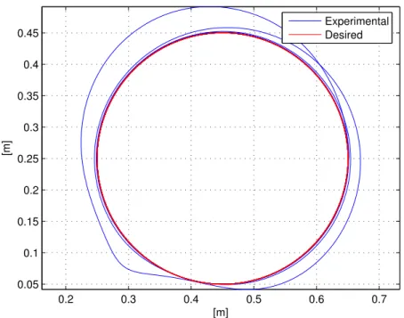
0.2 0.3 0.4 0.5 0.6 0.7 0.05 0.1 0.15 0.2 0.25 0.3 0.35 0.4 0.45 [m] [m] Experimental Desired
Figure 2.6 Actual and desired end-effector trajectory for the simulation. Experimental Results
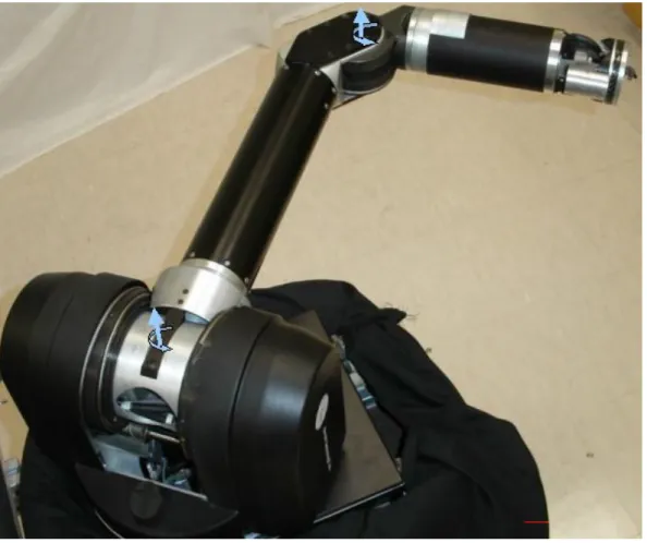
The developed controller was implemented on the Barrett whole arm manipula-tor (WAM). The WAM is a seven degree of freedom (d.o.f.), highly dexterous and back-drivable robotic manipulator. The objective of the experiment is to verify the performance of the developed adaptive controller. So to simplify the controller im-plementation, five joints of the robot were locked at fixed angles and the remaining links of the manipulator were used as a two d.o.f. planar robot manipulator (refer to Fig. 2.7). The dynamics of the robot in this planar configuration can be expressed as [61]: τ = M11 M12 M21 M22 ¨ θ1 ¨ θ2 + Vm11 Vm12 Vm21 Vm22 ˙ θ1 ˙ θ2 + fd1 0 0 fd2 ˙ θ1 ˙ θ2 (2.48)
Figure 2.7 Barrett Whole Arm Manipulator.
The elements of the inertia and centripetal-Coriolis matrices are defined as follows:
M11 = m1l2c1 +m2l2c2 +m2l21+ 2m2l1lc2cos (θ2) M12 = m2l2c2 +m2l1lc2cos (θ2) M21 = M12 M22 =m2l2c2 Vm11 = −m2l1lc2sin (θ2) ˙θ2 Vm12 = −m2l1lc2sin (θ2) ˙ θ1+ ˙θ2 Vm21 = m2l1lc2sin (θ2) ˙θ1 Vm22 = 0
where m1, m2 ∈ R denote the mass of the links, l1, l2 ∈ R denote the length of the links andlc1,lc2 ∈Rdenote the distance to the centre of mass. The termsfd1, fd2 ∈R in (2.48) denote the uncertain friction coefficients of the manipulator. The vector of
uncertain constant dynamic parametersφy ∈R14 was found to be:
φy =
[m1l1l2c1, m1l2l2c1, m1l2c1, m2l1lc22, m2l2l2c2, m2l2c2, m2l13,
m2l21, m2l21lc2, m2l1l2lc2, m2l21l2, m2l1lc2, fd1, fd2]T The control algorithm was written in “C++” and hosted on an AMD Athlon 1.2 GHz PC operating under QNX 6.2.1. Data logging and on-line gain tuning were performed using Qmotor 3.0 control software [65]. Data acquisition and control im-plementation were performed at a frequency of 1.0 kHz using the ServoToGo I/O board. Joint positions were measured using the optical encoders located at the mo-tor shaft of each axis. Joint velocity measurements were obtained using a filtered backwards difference algorithm.
Remark 4 The kinematics of the robotic system are assumed to be unknown. The task-space variable is assumed to be measured using an external sensor (e.g. a camera system or laser tracking could be used). To simplify the experiment, the task-space measurements were simulated by using the known kinematics of the robot (i.e., we artificially generate the task-space position measurements using the known forward kinematics). This kinematic information is used only to artificially generate the task-space signals and is not used to generate any other signals in the control algorithm.
The approximated Jacobian matrix which is used in the control implementation is defined as follows:
ˆ
Jp =
−ˆl1sin (θ1)−ˆl2sin (θ1+θ2) −ˆl2sin (θ1+θ2) ˆ
l1cos (θ1) + ˆl2cos (θ1+θ2) ˆl2cos (θ1+θ2)
where ˆJp ∈R2×2, ˆl1 and ˆl2 are estimates for the link lengths. The parameter vector ˆ φj ∈R2 is defined as: ˆ φj = ˆ l1 ˆl2 T
The true link lengths are l1 = 0.558 [m] and l2 = 0.291 [m]. We initialized the link length estimates to 75% of the true value. In cases where there is no information available about the link lengths, a best-guess could be used as an initial estimate of the link lengths.
The desired trajectory was defined as:
pd =
0.55 + 0.2 cos (2t) 0.25 + 0.2 sin (2t)
The initial position of the joints were, θ1(0) = 3.3◦, θ2(0) = 45.1◦, which corresponds to x(0) = 0.75 [m], y(0) = 0.25 [m] in the task-space. The control gains that yielded the best tracking performance were as follows:
k1 =diag{2.5,2.0}, kr =diag{80,40}
Γ1 =diag{8,1}, Γ2 =diag{20,45,10,500,1,3,8,15,20,5,500,25,20,20}
Remark 5 In this planar two degree of freedom example, there was no rotational
error ev(t); hence, the gain k2 is not used.
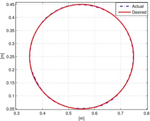
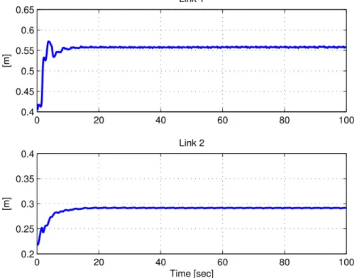
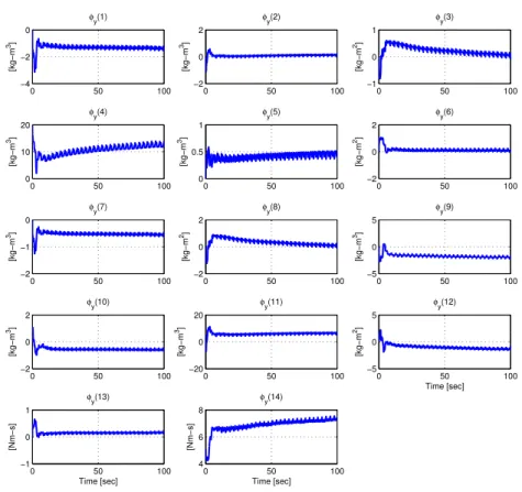
Fig. 2.8 shows the actual and desired task space trajectories for the last revolution. Fig. 2.9 shows the position tracking error, it is seen that within 10 seconds the tracking error converges to approximately ±2 [mm]. Fig. 2.10 and 2.11 show the link length estimates and the dynamic parameter estimates respectively. From Fig. 2.9, 2.10 and 2.11, it can be clear that the tracking error converges as the kinematic and dynamic parameters converge. Fig. 2.12 shows the control input torques to the two links of the Barrett WAM.
0.3 0.4 0.5 0.6 0.7 0.8 0.05 0.1 0.15 0.2 0.25 0.3 0.35 0.4 0.45 [m] [m] Actual Desired
Figure 2.8 Actual and desired end-effector trajectory (only the last revolution is shown).
0 20 40 60 80 100 −0.02 0 0.02 0.04 X−Axis [m] 0 20 40 60 80 100 −0.02 0 0.02 0.04 Time [sec] [m] Y−Axis
0 20 40 60 80 100 0.4 0.45 0.5 0.55 0.6 0.65 [m] Link 1 0 20 40 60 80 100 0.2 0.25 0.3 0.35 0.4 [m] Time [sec] Link 2
0 50 100 −4 −2 0 [kg−m 3] φ y(1) 0 50 100 −2 0 2 [kg−m 3] φ y(2) 0 50 100 −1 0 1 [kg−m 2] φ y(3) 0 50 100 0 10 20 [kg−m 3] φy(4) 0 50 100 0 0.5 1 [kg−m 3] φy(5) 0 50 100 −2 0 2 [kg−m 2] φy(6) 0 50 100 −2 −1 0 [kg−m 3] φy(7) 0 50 100 −2 0 2 [kg−m 2] φy(8) 0 50 100 −5 0 5 [kg−m 3] φy(9) 0 50 100 −2 0 2 [kg−m 3] φ y(10) 0 50 100 −20 0 20 [kg−m 3] φ y(11) 0 50 100 −5 0 5 [kg−m 2] Time [sec] φ y(12) 0 50 100 −1 0 1 [Nm−s] Time [sec] φ y(13) 0 50 100 4 6 8 [Nm−s] Time [sec] φ y(14)
0 20 40 60 80 100 −50 0 50 100 Link 1 [Nm] 0 20 40 60 80 100 −60 −40 −20 0 20 Link 2 Time [sec] [Nm]
CHAPTER 3
A NEURAL NETWORK CONTROLLER FOR CONTINUUM ROBOTS In this chapter a neural network based tracking controller is developed for a class of hyper-redundant robot manipulators, also known as “continuum” robot manipu-lators. The novelty of this work is the development of an efficient tracking controller for extensible continuum manipulators which can deal with a high level of uncer-tainty in the structure of the manipulators dynamic model. The proposed controller consists of a neural network feedforward component along with a nonlinear feedback component. Specifically, the design of the neural network component is based on the augmented back propagation algorithm [33], and it is used to compensate for the nonlinear uncertain dynamics of the continuum robot manipulator by leveraging the universal approximation properties of the neural network as a feedforward com-pensator. The feedback component utilized is a continuous nonlinear controller [40], which does not require any model information. The advantages of the proposed con-trol scheme compared to the previously mentioned works is that the concon-troller is continuous and asymptotic tracking can be proved without any prior knowledge of the robot dynamic model. Furthermore, the back propagation technique enables the neural network weight matrices to be estimated on-line very quickly based on the tracking error signal and without utilizing any prior training period. This technique is particularly useful for real time closed loop control.
This chapter is organized as follows, in the first section, the sensing and actuation of the OCTARM VI, which is a soft extensible continuum robot manipulator (see Fig. 3.1), are briefly discussed. Then some of the prior efforts to develop dynamic models for continuum robot manipulators are discussed and a model for the extensi-ble continuum manipulator is presented. In the next section the control objective is explicitly defined and the design of a controller with the neural network feedforward component is presented. To demonstrate the performance of the proposed controller with the neural network feedforward component, the controller was tested on the
OC-TARM. In the experimental results section, the performance of the controller without the neural network feedforward component is compared with that of the controller with the neural network feedforward component to illustrate the effectiveness of the proposed strategy.
Figure 3.1 OCTARM VI continuum manipulator grasping a ball in Clemson University’s robotics laboratory.
Robot Sensing and Actuation
The OCTARM VI manipulator [19, 24, 66], is a biologically inspired soft contin-uum manipulator resembling a trunk or tentacle. The OCTARM is significantly more versatile and adaptable than conventional robotic manipulators, capable of adaptive and dynamic manipulation in unstructured environments. To provide the desired dex-terity the OCTARM VI is constructed with high strain extensor air muscles called McKibben actuators. These actuators are constructed by covering latex tubing with a double helical weave, plastic mesh sheath [67]. These actuators provide a large strength to weight ratio and strain which are required for soft continuum manipula-tors.
The OCTARM VI (refer to Fig. 3.1) is divided into three sections, with each section consisting of three McKibben actuators. Each section is capable of two axis bending and extension hence allowing nine total degrees of freedom for the manipu-lator. The manipulator is pneumatically actuated through nine pressure regulators which maintain the pressure in the actuators at a desired value, set using an input voltage. The pressure regulators provide a linear relationship between the control voltage and the air pressure. By varying the air pressure to the actuators on a sec-tion the length and shape of the secsec-tion can be controlled.
The shape of the manipulator can be inferred in terms of curvatures and extensions by measuring the length of each of the nine actuators and using the forward kinematics described in [68]. In this work we are only concerned with developing an efficient low level controller which regulates the length of each of the actuators on the manipulator to follow a desired trajectory4.
Robot Dynamic Model
From a review of current literature, it is evident that the theory related to the dynamic modeling of continuum robot arms is still in its nascence with few published works available. Some of the previous research includes [69–71], where planar models of the continuum structure were considered, and [72, 73], where the authors develop a three dimensional dynamic model for an inextensible (constant length) continuum manipulator. As such, the complete dynamic modeling of variable length continuum robot arms remains an open research area. In [72], the developed dynamic model was shown to satisfy the familiar property that the continuum manipulators inertia matrix is symmetric and positive definite. With this in mind, in the development being considered we will assume that the dynamic model of a 9 DOF (degree of freedom) continuum robot manipulator can be described by the following expression.
M(q)¨q+N(q,q˙) =u (3.1)
4
Note that the desired trajectory for the lengths of each actuator could be specified directly in terms of the lengths or could be generated using the inverse kinematics described in [68].
where M(q) ∈ R9×9
represents the inertia matrix, N(q,q˙) ∈ R9 represents the re-maining dynamic terms such as centripetal, Coriolis and frictional forces , u(t)∈R9 represents the control input vector, and q(t), q˙(t), q¨(t) ∈ R9 represent the actuator length, velocity and acceleration respectively.
The subsequent development is based on the following assumptions
Assumption 1 The manipulators position q(t) and velocity q˙(t) are measurable.
Assumption 2 The dynamic terms denoted byM(q)andN(q,q˙)are unknown
non-linear functions of q(t) and q˙(t) which are second order differentiable and satisfy the
following properties
M(·),M˙ (·),M¨(·)∈ L∞ if q(t),q˙(t),q¨(t)∈ L∞ (3.2)
N(·),N˙(·),N¨(·)∈ L∞ if q(t),q˙(t),q¨(t),
...
q(t)∈ L∞. (3.3)
Assumption 3 The inertia matrixM(q)is symmetric and positive-definite, and sat-isfies the following inequalities
m1kξk2 ≤ξTM(q)ξ≤m2kξk2 ∀ξ ∈R9 (3.4)
where m1, m2 ∈ R are positive constants, and k·k denotes the standard Euclidean
norm.
Control design
As we have mentioned in the previous section, the dynamic modeling of extensible continuum manipulators remains an open research problem. The main focus of the control design in this section is to develop an efficient tracking controller which can deal with the high level of uncertainty in the structure of continuum robot’s dynamic model. The proposed control strategy consists of a neural network feedforward com-ponent and a nonlinear feedback comcom-ponent. The feedback comcom-ponent is based on prior work in [40], this controller is chosen because it leaves a lot of flexibility in the
design of the neural network feedforward component. The neural network feedforward component is then designed based on the back propagation algorithm in [33] to meet the boundedness requirements required by the feedback controller.
Feedback Controller
The control objective is to design a continuous controller which provides asymp-totic tracking of the actuator lengths and the desired actuator length trajectories in the sense that
q(t)→qd(t) ast→ ∞. (3.5)
To quantify the control objective, an error signal, denoted by e1(t) ∈ R9, is defined as follows
e1 ,qd−q. (3.6)
Furthermore, an auxiliary tracking error signal e2(t)∈R9 is defined as follows
e2 ,e˙1+λ1e1 (3.7)
where λ1 ∈ R+ is a control gain. For the closed loop error system development, we define a filtered tracking error signal r(t)∈R9 as follows
r ,e˙2+λ2e2 (3.8)
where λ2 ∈R+ is a control gain.
The dynamic model of the continuum robot is highly nonlinear and has an uncer-tain structure; hence, the strategy developed by Xian et al. [40], can be utilized for the controller. This controller is chosen because it is continuous, it does not require the dynamic model of the manipulator to be known and yet it provides semi-global asymptotic tracking. Specifically, the control objective described in (3.5) can be met with the following controller [40]
u(t) , (Ks+I)e2(t)−(Ks+I)e2(t0) + Z t t0 ˆ f(τ)dτ + Z t t0 (λ2(Ks+I)e2(τ) +βsgn(e2(τ)))dτ (3.9)
where u(t) ∈ R9 is the control input defined in (3.1), λ2 ∈ R+ is a control gain,
Ks, β ∈ R9
×9
are positive definite diagonal control gain matrices, ˆf(t) ∈ R9 is the neural network feedforward component, and sgn(·) : R9 7→ R9 denotes the vector signum function defined assgn(ξ) = [sgn(ξ1),· · · , sgn(ξ9)]T ∀ξ = [ξ1,· · · , ξ9]T ∈R9. As shown in [40], the controller presented in (3.9), provides semi-global asymptotic convergence of the actuator length tracking error, (i.e. ke1(t)k →0 as t → ∞). For brevity in this presentation, the stability analysis is omitted, for a complete analysis of the controller the reader is referred to [40].
Remark 1 The design of the neural network feedforward component, fˆ(t), is pre-sented in the subsequent section. The only restriction imposed on the neural network
component by the selection of the feedback controller in (3.9) is that fˆ(t) ∈ L∞, i.e.
the output from the neural network must be bounded.
Neural Network Feedforward Design
The neural network feedforward component ˆf(t) ∈ R9 is computed using a two layer network with 15 neurons. The weights are computed using a modified version of the back propagation algorithm presented in [33]. Given Remark 1, an important consideration regarding the design of the neural network feedforward component is that the output from the neural network must always be bounded (i.e. ˆf(t) ∈ L∞).
To this end the neural network component is defined as follows ˆ
f = ˆWTσ¯VˆTx. (3.10)
where ˆW(t)∈R15×9
and ˆV(t)∈R37×15
are estimated weight matrices, andx(t)∈R37 is the input vector to the neural network which is selected as
x= 1, qT d, q˙Td, q¨Td, ... qT d T (3.11) where qd(t),q˙d(t),q¨d(t), ...
qd(t) were defined a priori. The vector activation function
¯
σ(·)∈R15 7→R15 is defined as follows ¯
where ω = [ω1, ω2, · · · , ω15]T and σ(s) : R 7→ R is the sigmoid activation function defined as
σ(s) = 1
1 + exp(−s) . (3.13)
The gradient of the vector activation function, denoted by ¯σ′(·) ∈ R15×15
can be expressed in closed form as follows, [33]
¯
σ(ω)′ =diag{σ¯(ω)}[I−diag{σ¯(ω)}]. (3.14) If we were to design the weight update laws according to the augmented backpropa-gation algorithm [33], we would use the following update rules
˙ˆ
W =−κFkrkWˆ −Fσ¯′(·) ˆVTxrT +Fσ¯(·)rT
˙ˆ
V =−κGkrkWˆ +Gx¯σ′T(·) ˆW rT
whereκ ∈R+ is selected to be a small constant,F ∈R15×15
, G∈R37×37
are positive definite gain matrices,x(t) is the input vector defined in (3.11), andr(t) is the filtered tracking error signal defined in (3.8). Here, the filtered tracking error signal r(t) is required in the update laws which requires the measurement of the acceleration ¨q(t), and hence, is undesirable. To ensure that the weights generated from these laws are bounded, and that acceleration measurements are not required, we redefine the update laws as follows
˙ˆ W =−αwWˆ +γ1σ¯ ˆ VTx sat (e2+ζ)T (3.15) ˙ˆ V =−αvVˆ +γ2x h ¯ σ′VˆTxWˆsat (e2+ζ) iT (3.16) where αv, αw ∈ R+ are small constants, γ1, γ2 ∈ R+ are control gains which ef-fect the learning speed, the function sat(ξ) : R9 7→ R9 is defined as sat(ξ) = [sat(ξ1),· · ·,sat(ξ9)]T ∀ξ = [ξ1,· · · , ξ9]T ∈ R9 where sat(ξi) ∈ R ∀i = 1,· · · ,9 is the following saturation function
sat(ξi) = −ξmin if ξi ≤ −ξmin ξi if ξi >−ξmin or ξi < ξmax ξmax if ξi ≥ξmax
where ξmin, ξmax ∈R+ are constants. In (3.15) and (3.16) the auxiliary signal ζ(t)∈ R9 is an approximation (i.e. a dirty derivative operation) for the signal ˙e2(t) which is defined as follows
ζ = 1
ε(e2 −η) (3.17)
where ε ∈R+ is a small constant, and the signal η(t) ∈ R9 is updated according to the following expression
˙
η= 1
ε(e2−η). (3.18)
From equations (3.10)-(3.18) and the fact that the input vector to the neural network is bounded, it is easy to show that the weight matrices ˆW(t) and ˆV(t) are bounded, and hence, the output from the neural network, ˆf(t), is bounded.
Experimental Results
To verify the performance of the controller with the neural network feedforward component, the controller was implemented on the OCTARM VI continuum robot manipulator. In this section, we first provide a description of the control system for the OCTARM VI continuum robot manipulator, then experimental results are described which illustrate the effectiveness of the neural network feedforward tracking controller.
OCTARM Control System
Figure 3.2 shows an overview of the control system of the OCTARM. The con-trol system consists of a commercial off-the-shelf Pentium III EBX form-factor Single Board Computer (SBC) with two ServoToGo data acquisition boards which provide analog and digital I/O. The computer runs the QNX Neutrino real-time operating system and QMotor 3.0 [65], a real-time control software which facilitates online parameter tuning and data logging for the implemented control programs. Data ac-quisition and closed loop control were performed at a frequency of 500 Hz. There are nine pressure regulators, one for each actuator on the manipulator. The air pressure
Figure 3.2 Block diagram showing an overview of the OCTARM VI control system. for each actuator is determined by the neural network controller. The pressure spec-ified by the controller is converted to a corresponding voltage level (using a linear relationship between pressure and voltage) and this drives the pressure regulators which control the air flow to the actuators.
For closed loop control of the OCTARM VI manipulator accurate sensing of the actuator lengths is essential. To measure the length of each of the nine actuators, there are nine string encoders arranged around the base of section one (see Fig. 3.3). The cables from each of the string encoders run the entire length of the actuator they are assigned to measure. This configuration enables the length of each of the actuators on the OCTARM VI manipulator to be determined. Since the string encoders have a relatively low resolution, velocities obtained through differentiation of the position measurements are noisy; hence, a variable structure velocity observer [40], was utilized to obtain estimates of the velocity.
Trajectory Tracking Experiment Description
To test the low level controller with the neural network component given in (3.9), a sinusoidal trajectory was selected for the actuator lengths. Since, the three actua-tors on a section are 120 degrees apart mechanically, the desired trajectory for each
Figure 3.3 The OCTARM VI robotic manipulator.
actuator in a section is shifted 120 degrees in phase from the trajectory of the previous actuator in that section. The trajectory for section one was selected as follows
qd1k = lmin1 + (1−exp(−0.5t))l1 +3(1−exp(−0.5t))sin 0.03πt+ 2 3πk
where k = 1,2,3, qd1 = [qd11, qd12, qd13]∈R3 represents the desired trajectory for the actuators on section one,lmin1 ∈R represents the minimum lengths of the actuators on section one, andl1 = 8 [cm] is the initial extension of the actuators on section one. The initial extension was selected to keep the operating pressure close to its nominal value. For sections two and three, the initial extensions were l2 = 7 [cm], l3 = 5 [cm] and the frequency of the sinusoidal trajectory for each section was twice that of the previous section. The minimum and maximum lengths of the sections corresponding to the minimum pressure (0 psi) and maximum pressure (130 psi) respectively are physical limitations of the actuators and were found to be lmin1 = 28 [cm], lmin2 = 26.5 [cm], lmin3 = 32.5 [cm],lmax1 = 42 [cm], lmax2 = 44 [cm], lmax3 = 54 [cm].
Control Parameter Tuning
To test the effectiveness of the neural network feedforward component, we com-pared the performance of the controller in (3.9), with and without the neural network