An Optimization Approach for Localization
Refinement of Candidate Traffic Signs
Zhe Zhu, Jiaming Lu, Ralph Martin, and Shimin Hu,
Member, IEEE
Abstract—We propose a localisation refinement approach for candidate traffic signs. Previous traffic sign localisation ap-proaches which place a bounding rectangle around the sign do not always give a compact bounding box, making the subse-quent classification task more difficult. We formulate localisation as a segmentation problem, and incorporate prior knowledge concerning color and shape of traffic signs. To evaluate the effectiveness of our approach, we use it as an intermediate step between a standard traffic sign localizer and a classifier. Our experiments use the well-known GTSDB benchmark as well as our new CTSDB (Chinese Traffic Sign Detection Benchmark). This newly created benchmark is publicly available, and goes beyond previous benchmark datasets: it has over 5,000 high-resolution images containing more than 14,000 traffic signs taken in realistic driving conditions. Experimental results show that our localization approach significantly improves bounding boxes when compared to a standard localizer, thereby allowing a standard traffic sign classifier to generate more accurate classification results.
Index Terms—Traffic Sign Localization, Optimization, Graph Cut.
I. INTRODUCTION
T
RAFFIC signs are specially designed graphics which give instructions and information to drivers. Although different countries’ traffic signs vary somewhat in appearance, they share some common design principles. Traffic signs are divided according to function into different categories, in which each particular sign has the same generic appearance but differs in detail. This allows traffic sign recognition to be carried out as a two-phase task: detection and classification. The detection step focuses on localizing candidates for a certain traffic sign category, typically by placing a bounding box around regions believed to contain such a traffic sign. Classification then examines these regions to determine which specific kind of sign is present (if any).Two well known benchmarks are used to assess detection and classification separately. The GTSDB detection benchmark [1] consists of 900 images with resolution 1360×800, in which the size of traffic signs ranges from 16 to 128 pixels. The GT-SRB classification benchmark [2] contains more than 50,000 images, but here the objects of interest fill much of each image. Although various methods have achieved good performance
Z. Zhu, J. Lu and S. Hu are with the TNList, Tsinghua University, Bei-jing 100084, China. E-mail: [email protected],[email protected], [email protected].
R. R. Martin is with the School of Computer Science & Informatics, Cardiff University, UK. E-mail:[email protected].
on both detection and classification benchmarks, it is still a challenging task to recognize traffic signs in an image where the objects of interest occupy a small fraction of the whole image. There is still a significant gap between detection and classification, caused by inaccurate detection results: detected bounding boxes do not always enclose the sign as compactly as possible. The Jaccard similarity coefficient is often used to evaluate the effectiveness of a traffic sign detector, and in particular, in the GTSDB competition, candidates with Jaccard similarity greater than 0.6 were regarded as having correctly detected the sign. However, this criterion results in many inaccurate bounding boxes being regarded as correctly detecting the sign, yet such loose boxes provide a poor basis for classification.
Thus, in this paper, we propose a new localization refinement approach for candidate traffic signs. Our optimization ap-proach is intended for use as an intermediate step between an existing detection method and the classification step. Starting from an approximate bounding rectangle provided by some other detector, our approach is intended to give a more accurate bounding box. This step can significantly improve the detection quality, leading to better classification results. In [3] a radial symmetry detector [4] is used for fast detection of circular signs. Although it can accurately localize signs by using centroids, it works for circles only, and cannot be generalized to other shapes of traffic signs. Our approach is generic, and we do not need to design a detector for a particular shape. Our approach just uses a shape mask as a template to provide prior knowledge: for different shapes of traffic signs we just need to change the template. In Figure 1(a) the yellow rectangle marks the region detected by a well-trained cascade using (HoG features). Our approach more accurately localizes the traffic sign as illustrated in Figure 1(b). The final segmentation result is illustrated in Figure 1(c). We formulate localization refinement as a segmentation prob-lem using prior shape and color knowledge. The shape prior is provided in the form of planar templates of standard shape, as illustrated in Figure 2. Our approach encourages the segmented shape to appear similar to the pre-defined template, allowing for a homography transformation caused by camera projection. To provide a color prior, we note that traffic signs in a par-ticular category have a relatively fixed proportion of intrinsic colors. However, under different illumination conditions, these colors may look quite different, so setting color thresholds is impractical. Instead, we use a training set to train a Gaussian mixture model (GMMs) for each particular category of traffic signs to model expected foreground colors.
(a) (b) (c)
Fig. 1. Two examples of traffic sign localization: (a) Detection result using a cascaded detector (yellow rectangle). (b) Optimized detection result using our approach (green rectangle). (c) Segmentation result (white pixels).
(a) (b) (c) (d)
Fig. 2. Templates for the four most common shapes for traffic signs in China: (a) circle, (b) triangle, (c) inverted triangle, (d) octagon.
To demonstrate the utility of our approach, we use the Viola-Jones cascade framework [5] with HoG [6] and Haar [7] features, as well as a state-of-the-art convolutional neural network (CNN) based object detector—Fast R-CNN [8], as baseline detectors whose output we aim to improve upon. Fast R-CNN uses an image and a set of object proposals (e.g. obtained from selective search [9]) as input, and processes the whole image with several convolutional and max pooling layers to produce a feature map. Then for each proposal it extracts a fixed length feature vector which is fed to a sequence of fully connected layers. The final layer outputs softmax probability estimates for M object classes plus a background class. We use these detectors for two reasons: (i) the detectors can achieve good performance without any application specific modification, and there are publicly available implementations of the main steps, making it easy for others to reproduce our results, and (ii) HoG features are useful for capturing the overall shape of an object while Haar features work well for representing fine-scale textures. CNNs have proven successful in many object detection scenarios and generally outperform traditional detectors.
The rest of the paper is organized as follows: in Section II we give a brief review of related work. Our localization refinement algorithm is detailed in Section III. Experimental results are provided in Section IV while we draw conclusions in Section V.
II. RELATEDWORK
A. Traffic Sign Detection
Color and shape are two important cues used in traffic sign detection. Early work [10], [11] applied color thresholds to quickly detect regions having a high probability of containing traffic signs. Although color-based methods are fast, it is hard to set suitable thresholds suitable for a wide range of conditions, as different illumination leads to severe color differences. While requiring greater computation, shape-based methods are less sensitive to illumination variance, and so are more robust than color-based methods. Directly detecting shapes [3] and using shape features [12] are the two major approaches to shape-based detection. While directly detecting shapes can accurately locate shapes, there are two obvious dis-advantages. One is that different detectors are typically needed for different shapes, e.g. the algorithms for detecting triangles and circles are different. A second is the need to take into account the homography transformation between the projected traffic sign in an image and its standard template shape, which complicates direct shape detection. Training a shape detector using shape features is more robust than directly detecting shapes. To detect traffic signs in an image, a multi-scale sliding window scheme is used, and for each window a classifier such as SVM or AdaBoost decides whether it contains a traffic sign [12]. Although feature based shape detectors are more robust than direct shape detectors, the detected candidates are still not always accurately localized. Another way to detect traffic signs is to regard the regions containing traffic signs as maximally stable extremal regions [13], but this method needs manual selection of various thresholds.
B. Traffic Sign Classification
Various object recognition methods have been adapted to classify traffic signs. In [11] a Gaussian-kernel SVM is used for traffic sign classification. Lu et al. [14] used a sparse-representation-based graph embedding approach which outper-formed previous traffic sign recognition approaches. Recently, many works have used CNNs for traffic sign classification, such as the committee of CNNs approach [15], use of hinge loss trained CNNs [16] and multi-scale CNNs [17]. CNN based traffic sign classification methods can achieve excellent results, but to do so requires images (like those in existing clas-sification benchmarks) containing an approximately centered traffic sign that fills much of the image. To work well, classifi-cation relies on accurate detection and localisation of candidate traffic signs. Some works [10], [13] have tried to concatenate detection and classification, adding a normalization step which aims to accurately locate the detected candidates. However these normalization steps just rely on shape detectors and are not robust enough for real applications.
For other traffic sign detection and classification methods, a detailed survey can be found in [18].
C. Image segmentation
The core of our approach is to segment the foreground using prior knowledge of color and shape. Segmenting foreground from background in images is an important research topic in computer vision and computer graphics. Level set meth-ods [19], [20], [21] and graph cut methmeth-ods [22], [23] are two popular approaches. However, we concentrate on methods which have the potential to solve our specialised segmentation problem. To model segmentation using shape priors, Cremers et al. [19] include a level set shape difference term in Chan and Vese’s segmentation model [20]. However their method needs initialization of the shape at the proper location, totally covering the shape to segment, while a standard traffic sign detector only offers a rough position of the object, so is unsuitable for this purpose. To handle possible transformations between the shape template and the shape to segment, Chan et al. [21] incorporate four parameters in the shape distance function, representingxandytranslation, scale and orientation. These only permit similarity transformations between shapes, whereas we need to handle a homography.
In [24] foreground and background color GMMs are used for segmentation, but the models rely on a user-selected rectangular region of interest. Freedman et al. [22] require user input to estimate rotation and translation parameters and then find the scale factor by brute force, again only handling similarity transformations. Vu et al. [23] use normalization images [25] to align the segmented shape with the template shape, but this approach is very sensitive to noise, and it is only affine invariant. No current segmentation approach can simultaneously incorporate color and shape priors while allowing for a homography transformation.
III. LOCALIZATIONREFINEMENT VIAENERGY
MINIMIZATION
Given the image containing the traffic sign with an initial rough rectangle locating it, we aim to accurately localize the traffic sign by segmenting it precisely. Each sign is contained within a set of pixels of interest, a subregion in the image that contains the traffic sign, found by somewhat enlarging the result of a standard traffic sign detector. Restricting pro-cessing to this region for each sign significantly reduces the computation time.
Segmentation can be formulated as an energy minimization problem based on the following energy function:
E(L) =
∑
p∈P
Edata(Lp) +λsmooth
∑
{p,q}∈NEsmooth(Lp,Lq). (1)
The above equation is a Markov random field formulation with unary and pairwise cliques [26] weighted by λsmooth. L ={Lp|p ∈P} is a labeling of all pixels of interest in the image where Lp∈ {0,1}; 1 stands for foreground (i.e. belonging to the sign) and 0 stands for background.
The data term accumulates the cost of giving labelLpto each
pixel pwhile the smoothness term considers the pairwise cost
of giving neighbourhood pixels p and q labels Lp and Lq
respectively. The neighbourhood N is determined by 8-fold connectivity. The data term is further split into a color term and a shape term. The color term encourages assignment of foreground (or background) labels to pixels consistent with a pre-trained foreground (or background) color model. The shape term encourages the shape of the labeled foreground to be similar to the prior shape template. The smoothness term penalises low-contrast boundaries. We next give detailed explanations of these energy terms.
A. Data Term
The data term is defined as follows:
Edata(L,H) =Ecolor(L) +λshapeEshape(L,H), (2)
whereλshape controls the relative importance of its two
com-ponents. H is the homography transformation we must also estimate: see Section III-C.
1) Color Term: As in [24], we use GMMs to model the foreground and background color distributions in RGB color space. Both foreground and background have a GMM withK
components (choice ofK will be described later). The color term is defined as:
Ecolor(L) =
∑
p∈P,k∈{1,...,K}Dcolor(Lp,kp,Ip,θ) (3)
where Dcolor(Lp,kp,Ip,θ) is the cost of assigning label Lp
to pixel p and component kp to the GMM color model. Ip
is the RGB value of pixel p and θ is the GMM model. Following [24],Dcolor(Lp,kp,Ip,θ)is defined as:
Dcolor(Lp,kp,Ip,θ) =−logπ(Lp,kp) + 1 2log detΣ(Lp,kp)+ 1 2[Ip−µ(Lp,kp)] T Σ(Lp,kp)−1[Ip−µ(Lp,kp)]. (4) In the above equation,π(·),µ(·)andΣ(·)are respectively the mixture weighting, mean and covariance of the GMM model.
2) Shape Term: The shape term encourages the shape of the segmented image to be similar to a pre-defined shape template. To compute the distance between two shapes, we use the function defined in [21] for binary images:
Dshape(ψa,ψb) =
∑
p∈P(ψap(1−ψbp) + (1−ψap)ψpb), (5)
whereψa,ψbare two shapes given by binary images, and for
a pixel p,ψp is its binary value.
Since traffic signs are planar objects, a homography transfor-mation relates a particular traffic sign to its standard shape template. Taking the homography transformation into consid-eration, our shape term is defined as:
Eshape(L,H) =Dshape(L,Hψ), (6)
where L is the binary labeled image, H is the homography transformation to be estimated andψ is the pre-defined shape template.
B. Smoothness Term
The smoothness term encourages the segmentation boundary to follow high contrast boundaries in the image. In practice, the magnitude of the image gradient may be used as the contrast metric. Following [24], smoothness energy is defined as:
Esmooth(Lp,Lq) =
Lp−Lq
exp −β(Ip−Iq)2 (7)
whereβ is a constant (whose setting will be described later).
If two neighbouring pixels have the same label, then the cost is zero, and this term penalizes low contrast boundaries.
C. Iterative Optimization
Our goal is to minimize the energy function in Eqn. (1) to get the labelingLi. As the variableHus also unknown, we should
write Eqn. (1) as:
E(L,H) =
∑
p∈P Edata(Lp,H) +λsmooth∑
{p,q}∈N Esmooth(Lp,Lq). (8) Simultaneously finding L and H is difficult, so we use an iterative optimization approach. First, we just use the color term and smoothness term to get an initial segmentation result using graph cut [27]. We then estimate an initial homography transformation (see Section III-D). Then during each iteration, we do the following:• FixH and updateL. GivenH,L can be computed using graph cut.
• Fix L and update H. Given L, H can be estimated as described in Section III-D.
If the number of changed labels divided by the total number of pixels is less than the thresholdtdthen we regard the process as
having converged, and in any case we stop after a maximum of Tmax iterations. Examples of segmentation results during successive iterations can be found in the first 5 columns in Figure 9.
D. Homography Estimation
To estimate the homography given the shape template and current segmented result as target shape, we first sample Ns
points on each shape boundary and compute its shape context descriptor [28]. (This is a histogram describing the distribution of relative positions of other sample points). Given this pair of shape context descriptors, finding the correspondence between the shapes is a quadratic assignment problem. To robustly handle outliers, we follow the strategy in [12], and add dummy nodes for each shape. The problem can be solved efficiently using the algorithm in [29]. As we know that the transformation between the two shapes is a homography, we finally fit a homography transformation between the two point sets using RANSAC [30].
Fig. 3. Segmentation results with varying parameterr. Top left: source region of interest containing a triangle sign. Top right:r= 2. With this setting, the shape term is always weaker than the smoothness term, so segmentation is dominated by contrast. Bottom left:r= 4. The color term now plays a more important role in earlier iterations while the shape term dominates the energy in later iterations. Segmentation converges to the desired result. Bottom right:
r= 8. The shape term dominates the energy too soon and iteration fails to converge to the correct segmentation.
E. Implementation Details
1) Varying the Shape Weight during Iteration: During iterative optimization, since the initial shape is only a rough estimate, the color information should play a more important role in early iterations while the shape constraint should dominate the energy term in later iterations. We thus change the weight of the shape term during iteration, successively increasing it as follows:
λsi=wri−1, i∈[1,Tmax] (9)
In the above equation λsi is the shape weight during the ith iteration,wis the initial shape weight, and rcontrols its rate of increase.
2) Using the Initial Bounding Box: Although the initial input bounding box for each sign may not be accurate, it gives a rough position for the traffic sign. To be able to use it to initialize segmentation, we first enlarge it to twice its size to give a looser bounding box, which we assume will always completely cover the foreground object. Pixels outside it can be safely regarded as background pixels, and are given the maximum penalty for having a foreground label.
3) Parameter Settings: The parameter K in the energy term is set to 6, as most traffic signs have 2 or 3 dominant colors (e.g. prohibitory signs are typically white, red and black ). Following [24] we set λsmooth to 50 and β to 0.3. For
shape alignment, we setNs to 50 empirically. During iterative
optimization we settdto 0.001,wto 0.5,rto 4 andTmax to 5
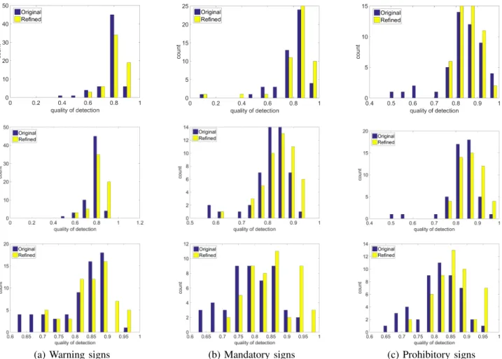
(a) Warning signs (b) Mandatory signs (c) Prohibitory signs
Fig. 4. Improvements in localization achieved for the three sign categories in GTSDB. Blue bars: quality of original detector. Yellow bars: quality of detection after refinement. Top to bottom: detectors using HoG features, Haar features and a Fast R-CNN detector. Corresponding statistics (median, mean and standard derivation of each histogram) are given in Table I.
TABLE I
QUALITY HISTOGRAM STATISTICS FOR ORIGINAL AND REFINED LOCALIZATION QUALITY USINGGTSDB Warning Mandatory Prohibitory median mean s.d. median mean s.d. median mean s.d. Original (HoG feature) 0.791 0.773 0.084 0.821 0.794 0.158 0.840 0.832 0.102 Refined (HoG feature) 0.838 0.826 0.073 0.845 0.820 0.140 0.868 0.864 0.050 Original (Haar Feature) 0.789 0.772 0.067 0.825 0.814 0.073 0.841 0.826 0.078 Refined (Haar feature) 0.827 0.819 0.068 0.846 0.844 0.062 0.861 0.867 0.052 Original (Fast R-CNN) 0.839 0.812 0.083 0.789 0.789 0.079 0.819 0.815 0.069 Refined (Fast R-CNN) 0.859 0.851 0.067 0.851 0.848 0.072 0.856 0.858 0.054
IV. EXPERIMENTS
We evaluate the effectiveness of our approach using two criteria: the improvement in localization, and the benefits to a subsequent classifier.
A standard detector provides its localization result in the form of an initial bounding box; we produce a refined bounding box. The quality of detection Qcan be assessed as
Q=| ∩(D,G)|/| ∪(D,G)|
where| · |denotes the number of pixels in a region, D is the detected traffic sign region, andGis the ground truth region. A quality of 0 means there is no overlap between the detected region and the ground truth, while 1 means perfect agreement. We compute this quality for the output of the standard detector and for the output of our approach, and for a series of test cases, make a detection quality histogram in steps of 0.1 between 0 and 1. We compare the histograms for the standard detector and for the results of our refinement approach, both visually, and by computing the median value, mean value and standard deviation for each histogram.
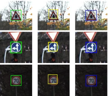
Fig. 5. Localization refinement results for examples from GTSDB. Rows: different categories of sign. Left: after refinement by our approach. Center: output of standard detector. Right: ground truth annotation.
Separately, to evaluate the benefits to a classifier of our approach, we cropped the detected traffic signs to the bounding box determined by a standard detector and our approach, and compared the classification performance of an appropriately trained classifier on test data.
Our experiments used two datasets used for evaluation: GTSDB and a newly created dataset which we call CTSDB (Chinese Traffic Sign Detection Benchmark). GTSDB is widely used in the research community for detection eval-uation. It contains 900 images with 43 classes of German traffic signs. Since the number of signs in each class is unbalanced, some classes have insufficient samples for training a classifier (it is intended for evaluating detection only), so we only used this dataset to evaluate improvement of localization quality. CTSDB has 5488 images in total, and was used both to evaluate localization quality and benefits to classifier were evaluated performance. Compared to GTSDB, CTSDB is a step forward. Firstly, it contains many more images and traffic signs; the image resolution is also higher than in GTSDB. Secondly, the images in this benchmark were captured in hundreds of different cities in China, under a wide range of illumination and lighting conditions corresponding to actual driving conditions. We are making this dataset publicly available, in the hope that the community will find it useful in future.
We carried out our experiments on a PC with an Intel i7 3770 CPU, an NVIDIA GTX 780Ti GPU and 8GB RAM. To detect the rough positions of the traffic signs, we used 3 different object detectors: a cascade detector with HoG features, a cas-cade detector with Haar features, and a Fast R-CNN detector. We implemented our algorithm using C++ and CUDA. For the shape matching step, we used a CUDA implementation of the parallel bipartite graph matching approach [31] which is the bottleneck in sequential implementation; for the graph
Fig. 6. Four views cropped from a panoramic image. Blue: front view. Red: left view. Yellow: right view. Green: back view.
cut step, we used the CUDA graph cut implementation [32] directly. Our localization refinement algorithm takes 15ms for a typical traffic sign, so can achieve about 67 fps.
A. Experiments on the GTSDB benchmark
To evaluate the improvement of localization when using the GTSDB benchmark, we again used the first 600 images for training and last 300 for testing. To enhance the robustness of the detector which provides our input, we used a data aug-mentation strategy: for each image we generated 18 samples using a random transformation by translating it in the range [−5,5]pixels, scaling it in the range[0.9,1.1]and rotating it in the range[−20◦,20◦]. This benchmark has 4 sign categories: ‘Prohibitive’, ‘Danger’, ‘Mandatory’ and ‘Other’; we ignore the ‘Other’ category as such signs have no fixed shapes. We considered three alternative detectors, a HoG feature based cascade detector, a Haar feature based cascade detector, and a Fast R-CNN detector. In each case, we trained 3 different detectors for the 3 target categories separately.
Quality histograms of unrefined and refined localization out-put are given in Figure 4 while statistics summarizing the histograms are provided in Table I. It can be seen that the distributions for the refined results have shifted closer to 1 than for the unrefined localisation, which is confirmed by the statistics in Table I: the refined results have higher median and mean quality, and a smaller spread compared to the unrefined results. Localization is improved by our refinement approach. We show three typical results in Figure 5, illustrating that our localization results (green rectangles) are closer to the ground truth (blue rectangles) than the standard detector output (yellow rectangles).
B. Experiments on the CTSDB benchmark
To evaluate the localization quality of our approach on other types of traffic signs as well as its benefit to the subse-quent classification task, we created a new, large, traffic sign benchmark which we call the Chinese Traffic Sign Detec-tion Benchmark. We collected 25000 360◦ panoramas from Tencent Street Views and cropped four sub-images: a front
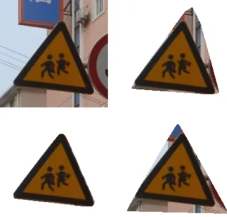
Fig. 7. Chinese traffic signs. Signs in yellow, red and blue boxes are warning, prohibitory and mandatory categories respectively. Greyed out signs do not appear in CTSDB.
view, left view, right view and back view: see Figure 6. These panoramas were captured in good weather conditions using 6 DSLR cameras, in more than 30 cities in China. Each cropped image has a resolution of 2048×2048. Each class of traffic signs is represented with large appearance variations in scale, rotation, illumination and occlusion. Our dataset is intended to be more realistic of practical scenarios than the images provided by earlier datasets. As some captured images contain no traffic signs, we hand-selected 5488 cropped images which contain traffic signs for manual annotation of location plus type of sign. We separated this benchmark into three subsets each containing the same number of traffic signs. For the detection experiment we pick two subsets as a training set and a testing set; in the classification experiment we performed cross validation by choosing two subsets as a training set and a testing subset each time. All warning, prohibitory and mandatory Chinese traffic signs are listed in Figure 7 (neglecting variants with different characters). More than half of these classes appeared in our benchmark. The total number of traffic signs in our benchmark is 14227. This dataset plus its detailed annotation will be made publicly available soon.
We first used this dataset to evaluate the localization quality of our approach as before. We selected a subset of the signs in each category with similar color and shape. In particular, while in the warning category, all signs have similar shape and colour, for the prohibitory category, we only considered signs with a red circle and diagonal bar. For the mandatory category, only blue circles with white foreground were selected. Similar testing was carried out as for the CTSDB benchmark; the results are shown in Figure 8 and Table II. Further results are shown in Figure 9, illustrating how our approach improves the localization quality for images in this benchmark. As was found for CTSDB, our refinement approach provides quality scores with a higher median and mean, and a lower standard
deviation, showing that our approach improves localization for the CTSDB benchmark. Note that while CNNs are currently popular for many tasks, the localization quality of Fast R-CNN is not actually better than that of the other approaches. This is because Fast R-CNN uses general object proposals, and the proposal generator does not perform well for small objects in large images such as traffic signs in our benchmark.
We also evaluated the extent to which classification per-formance can be improved by using our method to refine localisation. We picked the 4 specific kinds of sign in each category having the most images and trained classifiers. These classes are illustrated in Figure 10. The classifier was trained using the images in the training data part of the benchmark. Data augmentation was again performed as in Section IV-A. For classification, to filter out redundant proposals distributed around the traffic signs, non-maximum suppression was ap-plied to the initial proposals, and we manually discarded as unsuitable any candidates with no overlap with the ground truth bounding boxes. For the HoG features and Haar features, appropriately trained SVMs with a Gaussian kernel were used as classifiers, using the output bounding boxes of the previous detectors as the input. For Fast R-CNN, we trained a multi-class neural network as a classifier, using the top 1000 proposals from the selective search results.
Classification results achieved using the original candidates (after the above filtering), the candidates optimized by our approach, and user annotated bounding boxes are given in Ta-ble III. The results in Figure 8 and TaTa-ble III show how our re-fined bounding boxes lead to better classification performance. Since appearance variations exist in traffic signs between the training set and the testing set, and the user-provided bounding boxes are not entirely accurate, the classifier does not achieve 100% accuracy even when provided with the ground truth localisation.
(a) Warning signs (b) Mandatory signs (c) Prohibitory signs
Fig. 8. Improvements in localization achieved for the three sign categories in CTSDB. Blue bars: quality of original detector. Yellow bars: quality of detection after refinement.Top to bottom: detectors using HoG features, Haar features and a Fast R-CNN detector. Corresponding statistics (median, mean and standard derivation of each histogram) are given inn Table II.
TABLE II
QUALITY HISTOGRAM STATISTICS FOR ORIGINAL AND REFINED LOCALIZATION QUALITY USINGCTSDB Warning Mandatory Prohibitory median mean s.d. median mean s.d. median mean s.d. Original (HoG feature) 0.852 0.825 0.136 0.833 0.824 0.102 0.824 0.812 0.084 Refined (HoG feature) 0.872 0.850 0.106 0.864 0.848 0.094 0.845 0.838 0.062 Original (Haar feature) 0.796 0.781 0.069 0.850 0.835 0.084 0.840 0.824 0.097 Refined (Haar feature) 0.825 0.830 0.063 0.869 0.864 0.043 0.858 0.843 0.096 Original (Fast R-CNN) 0.750 0.767 0.081 0.793 0.799 0.075 0.753 0.776 0.073 Refined (Fast R-CNN) 0.800 0.834 0.059 0.846 0.847 0.073 0.809 0.820 0.075
C. The Benefit of Shape Constraints
The main difference between our approach and previous traffic sign segmentation methods is the use of shape constraints while estimating the pose of the shape. Segmenting foreground traffic signs in the practical scenarios using only color con-straints is not robust, because the distribution of foreground color has a limited range while the the background color can be arbitrary. Additional use of a shape constraint guarantees that our segmentation process converges to a predefined shape in some appropriate pose. Figure 11 shows some segmentation results with and without shape constraints. The second column
illustrates failures in segmentation caused by similar back-ground and foreback-ground colors. Adding shape constraints gives correct segmentation results (see the third column), as in the last few iterations the shape term becomes a hard constraint.
D. Limitations
We cannot guarantee that our approach will generate an accurate location in all cases. Our experiments showed that failures have three main causes: very low light levels (see Figure 12(a)), regions that have similar color or shape (see Figure 12(b)), and regions containing multiple signs (see
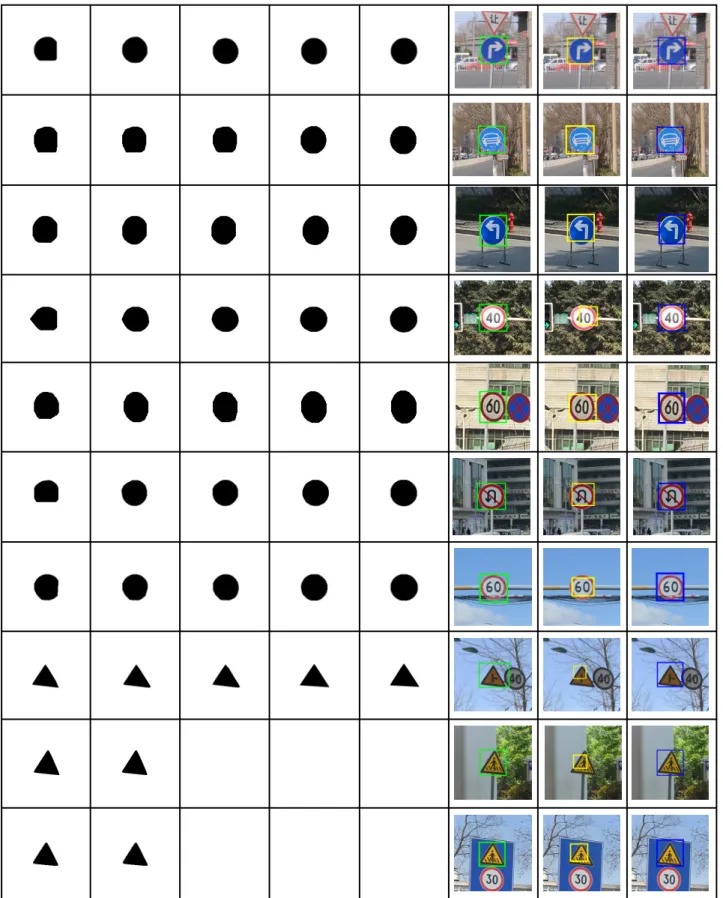
Fig. 9. Detection refinement results for various CTSDB images. Columns 1–5: segmentation results as iteration proceeds. Column 6: our localization results (green rectangles). Column 7: unrefined input from the cascade detector (yellow rectangles). Column 8: ground truth annotations (blue rectangles).
Fig. 10. Examples showing the 4 most frequent classes of sign for each of the 3 categories in the CTSDB benchmark.
TABLE III
CLASSIFICATION ACCURACY ACHIEVED BY PRESENTING A CLASSIFIER WITH DIFFERENT BOUNDING BOXES
Warning Mandatory Prohibitory Original (HoG feature) 82.76% 96.15% 86.36% Refined (HoG feature) 93.10% 100.00% 97.27% User-provided (HoG feature) 94.83% 100% 99.55% Original (Haar feature) 89.50% 92.05% 94.45% Refined (Haar feature) 90.60% 99.3% 98.28% User-provided (Haar feature) 92.41% 99.3% 100.00% Original (Fast R-CNN) 84.67% 87.50% 82.49% Refined (Fast R-CNN) 97.52% 99.30% 100% User-provided (Fast R-CNN) 100% 99.3% 100%
Fig. 11. Importance of shape constraints in segmentation, when the back-ground has similar color to the sign. Left: source image. Center: segmenta-tion result without shape constraints. Right: segmentasegmenta-tion result with shape constraints.
(a) (b) (c)
Fig. 12. Limitations: (a) convergence failure under low illumination, (b) confusion of similar shapes with similar color (the sky area is approximately circular at top left), (c) convergence on wrong sign given multiple adjacent signs.
Figure 12(c)). The energy minimization process in the seg-mentation step may not converge under poor illumination, in which case we retain the initial location. We also constrain the transformation relating the bounding box of the segmented result and the initial bounding box: the offset in x and y
directions must not exceed half of the initial width and height, the scale should lie in the range [0.65,1.5] and the rotation should not exceed 45◦. These constraints allow us to discard obviously incorrect interpretations. Another limitation of our approach is that it requires the output of a sufficiently good coarse location detector as input. If the input contains no signs, our approach will clearly fail.
V. CONCLUSIONS
This paper has given a localization refinement approach for candidate traffic signs. Color and shape priors are utilized in an iterative optimization approach to accurately segment the traffic signs as foreground objects. We have shown the effectiveness of our approach by comparing the localization quality of a cascade detector using HoG feature or Haar features, as well as the advantages of our approach when using CNNs: results using the GTSDB and CTSDB benchmarks show that our approach can improve localization quality. We have also shown that improved localization can lead to better classification using the CTSDB benchmark. While CNNs perform better than traditional detectors and classifiers, our approach still has the ability to further improve performance in this case too by giving more accurate bounding boxes. We have also provided CTSDB as a benchmark for further work in this field.
REFERENCES
[1] S. Houben, J. Stallkamp, J. Salmen, M. Schlipsing, and C. Igel, “Detection of traffic signs in real-world images: The german traffic sign detection benchmark,” in Neural Networks (IJCNN), The 2013 International Joint Conference on, Aug 2013, pp. 1–8.
[2] J. Stallkamp, M. Schlipsing, J. Salmen, and C. Igel, “Man vs. computer: Benchmarking machine learning algorithms for traffic sign recognition,”
Neural Networks, no. 0, pp. –, 2012.
[3] N. Barnes, A. Zelinsky, and L. Fletcher, “Real-time Speed Sign De-tection using the Radial Symmetry Detector,” IEEE Transactions on Intelligent Transport Systems, 2008.
[4] G. Loy and A. Zelinsky, “Fast radial symmetry for detecting points of interest,”Pattern Analysis and Machine Intelligence, IEEE Transactions on, vol. 25, no. 8, pp. 959–973, Aug 2003.
[5] P. Viola and M. Jones, “Rapid object detection using a boosted cascade of simple features,” inComputer Vision and Pattern Recognition, 2001. CVPR 2001. Proceedings of the 2001 IEEE Computer Society Confer-ence on, vol. 1, 2001, pp. I–511–I–518 vol.1.
[6] N. Dalal and B. Triggs, “Histograms of oriented gradients for human detection,” inComputer Vision and Pattern Recognition, 2005. CVPR 2005. IEEE Computer Society Conference on, vol. 1, June 2005, pp. 886–893 vol. 1.
[7] C. P. Papageorgiou, M. Oren, and T. Poggio, “A general framework for object detection,” in Computer Vision, 1998. Sixth International Conference on, Jan 1998, pp. 555–562.
[8] R. Girshick, “Fast R-CNN,” inProceedings of the International Confer-ence on Computer Vision (ICCV), 2015.
[9] J. R. R. Uijlings, K. E. A. van de Sande, T. Gevers, and A. W. M. Smeul-ders, “Selective search for object recognition,”International Journal of Computer Vision, vol. 104, no. 2, pp. 154–171, 2013.
[10] C. Bahlmann, Y. Zhu, V. Ramesh, M. Pellkofer, and T. Koehler, “A system for traffic sign detection, tracking, and recognition using color, shape, and motion information,” inIntelligent Vehicles Symposium, 2005. Proceedings. IEEE, June 2005, pp. 255–260.
[11] S. Maldonado-Bascon, S. Lafuente-Arroyo, P. Gil-Jimenez, H. Gomez-Moreno, and F. Lopez-Ferreras, “Road-sign detection and recognition based on support vector machines,”Intelligent Transportation Systems, IEEE Transactions on, vol. 8, no. 2, pp. 264–278, June 2007. [12] M. Mathias, R. Timofte, R. Benenson, and L. V. Gool, “Traffic sign
recognition - how far are we from the solution?” in Proceedings of IEEE International Joint Conference on Neural Networks (IJCNN 2013), August 2013.
[13] A. Martinovic, G. Glavas, M. Juribasic, D. Sutic, and Z. Kalafatic, “Real-time detection and recognition of traffic signs,” inMIPRO, 2010 Proceedings of the 33rd International Convention, May 2010, pp. 760– 765.
[14] K. Lu, Z. Ding, and S. Ge, “Sparse-representation-based graph em-bedding for traffic sign recognition.”IEEE Transactions on Intelligent Transportation Systems, vol. 13, no. 4, pp. 1515–1524, 2012. [15] D. C. Ciresan, U. Meier, J. Masci, and J. Schmidhuber, “A committee
of neural networks for traffic sign classification,” inInternational Joint Conference on Neural Networks, 2011, pp. 1918–1921.
[16] J. Jin, K. Fu, and C. Zhang, “Traffic sign recognition with hinge loss trained convolutional neural networks,”IEEE Transactions on Intelligent Transportation Systems, vol. 15, no. 5, pp. 1991–2000, 2014. [17] P. Sermanet and Y. LeCun, “Traffic sign recognition with multi-scale
convolutional networks,” inNeural Networks (IJCNN), The 2011 Inter-national Joint Conference on, July 2011, pp. 2809–2813.
[18] A. Mogelmose, M. M. Trivedi, and T. B. Moeslund, “Vision-based traffic sign detection and analysis for intelligent driver assistance systems: Per-spectives and survey.”IEEE Transactions on Intelligent Transportation Systems, vol. 13, no. 4, pp. 1484–1497, 2012.
[19] D. Cremers, N. Sochen, and C. Schn¨orr, “Towards Recognition-based Variational Segmentation Using Shape Priors and Dynamic Labeling,” in
Scale-Space Methods in Computer Vision, L. D. Griffin and M. Lillholm, Eds., vol. 2695. Isle of Skye: Springer, 2003, pp. 388–400. [20] T. F. Chan and L. A. Vese, “Active contours without edges,”Trans. Img.
Proc., vol. 10, no. 2, pp. 266–277, Feb. 2001.
[21] T. Chan and W. Zhu, “Level set based shape prior segmentation,” in
Computer Vision and Pattern Recognition, 2005. CVPR 2005. IEEE Computer Society Conference on, vol. 2, June 2005, pp. 1164–1170 vol. 2.
[22] D. Freedman and T. Zhang, “Interactive graph cut based segmentation with shape priors,” inComputer Vision and Pattern Recognition, 2005. CVPR 2005. IEEE Computer Society Conference on, vol. 1, June 2005, pp. 755–762 vol. 1.
[23] N. Vu and B. Manjunath, “Shape prior segmentation of multiple objects with graph cuts,” in Computer Vision and Pattern Recognition, 2008. CVPR 2008. IEEE Conference on, June 2008, pp. 1–8.
[24] C. Rother, V. Kolmogorov, and A. Blake, “”grabcut”: Interactive fore-ground extraction using iterated graph cuts,” ACM Trans. Graph., vol. 23, no. 3, pp. 309–314, Aug. 2004.
[25] S.-C. Pei and C.-N. Lin, “Image normalization for pattern recognition,”
Image and Vision Computing, vol. 13, no. 10, pp. 711 – 723, 1995. [26] D. M. Greig, B. T. Porteous, and A. H. Seheult, “Exact maximum a
posteriori estimation for binary images,”Journal of the Royal Statistical Society. Series B (Methodological), vol. 51, no. 2, pp. 271–279, 1989. [27] Y. Boykov and G. Funka-Lea, “Graph cuts and efficient n-d image
segmentation,”International Journal of Computer Vision, vol. 70, no. 2, pp. 109–131, 2006.
[28] S. Belongie, J. Malik, and J. Puzicha, “Shape matching and object recognition using shape contexts,” IEEE Trans. Pattern Anal. Mach. Intell., vol. 24, no. 4, pp. 509–522, Apr. 2002.
[29] R. Jonker and A. Volgenant, “A shortest augmenting path algorithm for dense and sparse linear assignment problems,”Computing, vol. 38, no. 4, pp. 325–340, Nov. 1987.
[30] M. A. Fischler and R. C. Bolles, “Random sample consensus: A paradigm for model fitting with applications to image analysis and automated cartography,”Commun. ACM, vol. 24, no. 6, pp. 381–395, Jun. 1981.
[31] C. N. Vasconcelos and B. Rosenhahn,Bipartite Graph Matching Compu-tation on GPU. Berlin, Heidelberg: Springer Berlin Heidelberg, 2009, pp. 42–55.
[32] “Graph cuts with cuda,” http://www.nvidia.com/content/GTC/ documents/1060 GTC09.pdf, accessed: 2016-06-30.
Zhe Zhu is a PhD student in the Department of Computer Science and Technology, Tsinghua Uni-versity. Before that, he received his bachelor’s degree in Wuhan University in 2011. His research interests in Computer Vision and Computer Graphics.
Jiaming Lu is an undergraduate student in the Department of Computer Science and Technology, Tsinghua University. His research interests in Com-puter Vision.
Ralph Martin is currently a Professor at Cardiff University. He obtained his PhD degree in 1983 from Cambridge University. He has published more than 250 papers and 14 books, covering such topics as solid and surface modeling, intelligent sketch input, geometric reasoning, reverse engineering, and various aspects of computer graphics. He is a Fellow of the Learned Society of Wales, the Institute of Mathematics and its Applications, and the British Computer Society. He is on the editorial boards of Computer Aided Design, Computer Aided Geomet-ric Design, GeometGeomet-ric Models, the International Journal of Shape Modeling, CAD and Applications, and the International Journal of CADCAM. He was recently awarded a Friendship Award, China’s highest honor for foreigners.
Shimin Hureceived the PhD degree from Zhejiang University in 1996. He is currently a professor in the department of Computer Science and Technology, Tsinghua University, Beijing. His research interests include digital geometry processing, video process-ing, renderprocess-ing, computer animation, and computer-aided geometric design. He is associate Editor-in-Chief of The Visual Computer, associate Editor of IEEE Transactions on Visualization and Com-puter Graphics, ComCom-puter & Graphics and ComCom-puter Aided Design.