University of Zurich Main Library Strickhofstrasse 39 CH-8057 Zurich www.zora.uzh.ch Year: 2010
The potential of modelbased recursive partitioning in the social sciences -Revisiting Ockham’s Razor
Kopf, Julia ; Augustin, Thomas ; Strobl, Carolin
Abstract: A variety of new statistical methods from the field of machine learning have the potential to offer new impulses for research in the social, educational and behavioral sciences. In this article we focus on one of these methods: model-based recursive partitioning. This algorithmic approach is reviewed and illustrated by means of instructive examples and an application to the Mincer equation. For readers unfamiliar with algorithmic methods, the explanation starts with the introduction of the predecessor method classification and regression trees. With respect to the application and interpretation of model-based recursive partitioning, we address the principle of parsimony and illustrate that the model-model-based recursive partitioning approach can be employed to test whether a postulated model is in accordance with Ockham’s Razor or whether relevant covariates have been omitted. Finally, an overview of available statistical software is provided to facilitate the applicability in social science research.
Posted at the Zurich Open Repository and Archive, University of Zurich ZORA URL: https://doi.org/10.5167/uzh-67143
Published Research Report Published Version
Originally published at:
Kopf, Julia; Augustin, Thomas; Strobl, Carolin (2010). The potential of model-based recursive partition-ing in the social sciences - Revisitpartition-ing Ockham’s Razor. München: University of Munich - Department of Statistics.
The Potential of Model-Based Recursive
Partitioning in the Social Sciences –
Revisiting Ockham’s Razor
Technical Report Number 88, 2010 Department of Statistics
University of Munich
partitioning in the social sciences –
Revisiting Ockham’s Razor
JULIA KOPF Ludwig-Maximilians-Universit¨at M¨unchen THOMAS AUGUSTIN Ludwig-Maximilians-Universit¨at M¨unchen CAROLIN STROBL Ludwig-Maximilians-Universit¨at M¨unchen
Abstract: A variety of new statistical methods from the field of machine learn-ing have the potential to offer new impulses for research in the social, educa-tional and behavioral sciences. In this article we focus on one of these methods: model-based recursive partitioning. This algorithmic approach is reviewed and illustrated by means of instructive examples and an application to the Mincer equation. For readers unfamiliar with algorithmic methods, the explanation starts with the introduction of the predecessor method classification and regres-sion trees. With respect to the application and interpretation of model-based recursive partitioning, we address the principle of parsimony and illustrate that the model-based recursive partitioning approach can be employed to test whether a postulated model is in accordance with Ockham’s Razor or whether relevant covariates have been omitted. Finally, an overview of available statistical soft-ware is provided to facilitate the applicability in social science research.
Keywords: model-based recursive partitioning; structural change; parsimony; classification and regression trees (CART); algorithmic methods; data analysis
1. Introduction
The aim of this paper is to demonstrate the potential of model-based recursive partitioning (Zeileis, Hothorn, and Hornik 2008), a new statistical method from the field of machine learning, for applications in the social sciences. In particular, we will point out that this algorithmic method provides a powerful tool to evaluate whether relevant covariates have been omitted in a statistical model and, therefore, whether a theoretically postulated model is in conflict with Ockham’s Razor. As a prototypical example the method is employed for evaluating the appropriate-ness of the so called Mincer equation (Mincer 1974), which explains different in-come levels through rates of return from schooling and work experience by means of a linear model. The analysis relies on data of the German Socio-Economic Panel Study (SOEP) from 2008, provided by DIW Berlin (German Institute for Economic Research).
Model-based recursive partitioning can be considered as an alternative to stan-dard multiple regression approaches and is based on the successive segmentation of the sample used: the data are split further as long as different groups of obser-vations still display substantially different values of the estimated parameters of the statistical model of interest.
For example, in our investigation of the Mincer equation we will see that the intercept and the estimated coefficient for further education vary across groups of men and women working full-time in east or west Germany. Thus additional sociological and economic theories, such as discrimination in labor markets (e.g. Aigner and Cain 1977; Phelps 1972), need to be considered for explaining these differences.
The method of model-based recursive partitioning forms an advancement of clas-sification and regression trees, which are widely used in life sciences (cf. e.g. Hann¨over, Richard, Hansen, Martinovich, and Kordy 2002; Kitsantas, Moore, and Sly 2007; Romualdi, Campanaro, Campagna, Celegato, Cannata, Toppo, Valle, and Lanfranchi 2003; Zhang, Yu, Singer, and Xiong 2001). Classification and re-gression trees will be summarized briefly in the following section, beginning with an informal description of the resulting tree-structure. After some technical de-tails of classification and regression trees are reviewed, in Section 3 the advanced method of model-based recursive partitioning is addressed, firstly by pointing out the main differences and similarities to classification and regression trees. The
review of model-based recursive partitioning will be continued by interpreting an instructive example and recapitulating the statistical background. To facilitate the use of this powerful algorithmic method in the social sciences, this article highlights the interpretation with regard to the principle of parsimony in the con-text of model construction (Section 4). Moreover, the application to the Mincer equation in Section 5 demonstrates the potential of model-based recursive parti-tioning in empirical research. For further research the available statistical software is indicated in Section 6.
In summary, in this paper we show how model-based recursive partitioning al-lows to decide whether a postulated model fails to describe the whole sample in a suitable way, because the method may detect varying parameter estimates in different subgroups of the sample. Model-based recursive partitioning therefore offers a synthesis of the theory-based and the data-driven approach. In particu-lar, it can be used for detecting violations of Ockham’s Razor. If subgroups with different parameter estimates are found, the postulated model is too simple and not appropriate for the entire sample.
2. Classification and regression trees
Classification and regression trees (cf. e.g. Breiman, Friedman, Olshen, and Stone 1984) are based on a purely data-driven paradigm. Without referring to a concrete statistical model, they search recursively for groups of observations with similar values of the response variable by building a tree structure. If the response is categorical, one refers to classification trees; if the response is continuous, one refers to regression trees. The basic principles of this approach will be explained by means of an exemplary application in the following section.
2.1. Basic principles of classification and regression trees
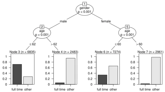
As a first example, we consider the respondents of the SOEP study 2008 (see Wagner, Frick, and Schupp 2007, for details about SOEP). In this data set, groups of subjects vary with respect to whether they participate in full-time labor or not (the latter including all categories like part-time or marginally employment, civil or military service, vocational training and unemployment labeled here as ‘other’). These groups can be described by means of covariates, such as age and gender.
The covariates (here: age and gender), together with the response variable (full time or other), are handed over to the algorithm. The resulting tree-structure is displayed in Figure 1. gender p < 0.001 1 male female age p < 0.001 2 ≤62 >62 Node 3 (n = 6835)
full time other 0 0.2 0.4 0.6 0.8 1 Node 4 (n = 2483)
full time other 0 0.2 0.4 0.6 0.8 1 age p < 0.001 5 ≤60 >60 Node 6 (n = 7274)
full time other 0 0.2 0.4 0.6 0.8 1 Node 7 (n = 2961)
full time other 0 0.2 0.4 0.6 0.8 1
Figure 1: Classification tree: Assessing different frequencies of full-time jobs in Germany (SOEP 2008). The resulting tree-structure shows varying par-ticipation rates in full-time labor in three splits according to the covari-ates gender and age.
From the entire sample of about 19,553 respondents living in private households, the covariate with the highest association (for technical details see Section 2.2) to the response is chosen for the first split. It is the participant’s gender, and, thus, 9,318 male respondents (represented in the left branch) are separated from the rest of the sample (10,235 female respondents, represented in the right branch). In the next step the male group is further diversified: it is split into two new subgroups, over the age of 62 or not (node 3 and node 4). Figure 1 also shows that the majority of women in the lower age group respond differently (node 6) compared to those in node 7. Here we stop the algorithm for simplicity.
The respective cutpoint for these splits depends on the type of the covariate: while gender has only two categories – male and female – and thus offers only one cutpoint, referring to age the algorithm must also find the ‘best’ cutpoint within this variable. This optimal cutpoint turns out to be located at the threshold of
gender p < 0.001 1 male female age p = 0.004 2 ≤43 >43 Node 3 (n = 236) 0 500 1000 1500 2000 2500 Node 4 (n = 147) ● ● ● ● ● ● ● ● ● ● ● ● ● ● ● ● ● ● ● ● ● ● ● ● ● ● ● ● ● 0 500 1000 1500 2000 2500 marital p < 0.001 5
single{mar., mar.s, div., wid.}
Node 6 (n = 207) 0 500 1000 1500 2000 2500 Node 7 (n = 360) ● ● ● ● ● ● ● ● ● ● ● ● ● ● ● ● ● 0 500 1000 1500 2000 2500
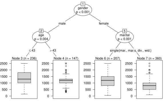
Figure 2: Regression tree: Assessing different requested incomes of unemployed respondents (SOEP 2008). Three different levels are obtained in groups related to gender, age and marital status.
62 years for the male subsample and 60 years for the female subsample (technical details are given below).
The resulting tree-structure is interpreted easily and shows groupwise frequencies for full-time and non-full-time workers in the end nodes: the left node indicates that the majority of men up to 62 years in Germany work full-time, while the ma-jority of women up to 60 do not. Women over 60 years are hardly ever employed full-time. The tree-structure in this example represents an interaction effect be-tween gender and age (see e.g. Strobl, Malley, and Tutz 2009, for details on the interpretation of main effects and interactions in classification trees).
In contrast to this classification problem, regression trees focus on continuous response variables. Instead of regarding the frequencies of the categories, groups with different average response values are separated and visualized, e.g. by means of box plots (like in Figure 2). These groups are again detected automatically. In this example the regression tree searches for different patterns of the (outlier adjusted) requested income at which 950 unemployed respondents would take a job
(outliers are defined as participants with a requested income higher than the third quartile plus 1.5 times interquartile range). Additional covariates are handed over to the algorithm are gender, age, nationality (nation) and marital status (marital). Figure 2 again shows the first split in the variable gender (node 1). The second split in the male subsample is again related to age (node 3 and node 4), while the third split in the female subsample is associated with marital status (node 6 and node 7). The cutpoint in a categorical variable is chosen automatically in an optimal way from all possible combinations of categories. Here the requested mean income is associated with marital status, in particular the request of female singles differs from the other categories (married, married but separated, divorced and widowed). The latter categories have smaller values of the requested income
(median xmed = 800, mean x= 870) than female singles (xmed = 1200, x= 1166),
who seem to be in the same magnitude as men over 43 years (xmed = 1200, x =
1159). The highest average of requested income occurs within the male subsample
up to the age of 43 years (node 3, xmed = 1300, x = 1349). After these three
splits, all of the determined groups are homogeneous enough to let the algorithm come to a stop, without further splitting, e.g. according to the nationality of the respondent. This exemplifies another attractive feature of partitioning methods: they implicitly perform a flexible variable selection.
A more detailed description of the technical procedure underlying classification and regression trees is given in the next section.
2.2. Some technical details
Classification trees search for different patterns in the response variable according to the available covariates. Since the sample is divided in rectangular partitions defined by values of the covariates and since the same covariate can be selected for multiple splits, classification trees can assess even complex interactions, non-linear and non-monotone patterns.
The structure of the underlying data-generating process is not specified in advance, but is determined in an entirely data-driven way. These are the key distinctions between classification and regression trees, and classical regression models. The approaches differ, firstly, with respect to the functional form of the relationship that is limited to e.g. linear influence of the covariates in most parametric re-gression models and, secondly, with respect to the pre-specification of the model
equation in parametric models.
Historically, the foundations for classification and regression trees were first de-veloped in the sixties as Automatic Interaction Detection (Morgan and Sonquist 1963). Later the most popular algorithms for classification and regression trees were developed by Quinlan (1993) and Breiman et al. (1984). Here we concen-trate on a more recent framework by Hothorn, Hornik, and Zeileis (2006b), which is based on the theory of conditional inference developed by Strasser and Weber (1999). The major advantage of this approach is that it avoids two fundamen-tal problems of earlier algorithms for classification and regression trees: variable selection bias and overfitting (cf. e.g. Strobl et al. 2009).
The algorithm of Hothorn et al. (2006b) for binary recursive partitioning can be described in three steps: firstly, beginning with the whole sample, the global null hypothesis that there is no relationship between any of the covariates and the response variable is evaluated. If no violation of the null hypothesis is detected, the procedure stops. If, however, a significant association is discovered, the variable with the largest association is chosen for the split. Secondly, the best cutpoint in this variable is determined and used to split the sample into two groups according to values of the selected covariate. Then the algorithm recursively repeats the first two steps in the subsamples until there is no further violation of the null hypothesis, or a minimum number of observations per node is reached.
In the following, we briefly summarize which covariates can be analyzed using classification and regression trees, how variables are selected for splitting and how the cutpoint is chosen.
2.2.1. The response variable in the end nodes
As outlined in the previous section, classification trees search for groups of similar response values with respect to a categorical dependent variable, whereas regres-sion trees focus on continuous variables. Hothorn et al. (2006b) stress that their conditional inference framework can be applied beyond that to situations of ordi-nal, censored survival times and multivariate response variables.
Within the resulting tree-structure, all respondents with the same covariate values – represented graphically in one end node – obtain the same prediction for the response, i.e. the same class membership for categorical responses or the same value for continuous response variables.
2.2.2. Selection of splitting variables
The next question is how the variables for the potential splits are chosen and how the related cutpoints can be obtained. As outlined above, Hothorn et al. (2006b) provide a statistical framework for tests applicable to various data situations. In the binary recursive partitioning algorithm, each iteration is related to a current data set (beginning with the whole sample), where the variable with the highest association is selected by means of permutation tests as described in the following. The usage of permutation tests allows for evaluating the global null hypothesisH0 that none of the covariates has an influence on the dependent variable. IfH0 holds (in other words, if the independence between any of the covariatesZj (j = 1, . . . , l)
and the dependent variableY cannot be rejected), the algorithm stops. Therefore
the statistical test acts both for variable selection and as a stopping criterion. Otherwise the strength of the association between the covariates and the response variable is measured in terms of the p-value that corresponds to the test of the par-tial null hypothesis that the specific covariate is not associated with the response. Thus, the variable with the smallest p-value is selected for the next split. The advantage of this approach is that the p-value criterion guarantees an unbiased variable selection regardless of the scales of measurement of the covariates (cf. e.g. Hothorn et al. 2006b; Strobl, Boulesteix, and Augustin 2007; Strobl et al. 2009). Permutation tests are constructed by evaluating the test statistic for the given
data under H0. Monte-Carlo or asymptotic approximations of the exact
null-distribution are employed for the computation of the p-values (see Hothorn, Hornik, van de Wiel, and Zeileis 2006a; Hothorn et al. 2006b; Strasser and Weber 1999, for more details).
2.2.3. Selection of the cutpoints
After the variable for the split has been selected, we need a cutpoint within the range of the variable to find the subgroups that show the strongest difference in the response variable. In the procedure described here, the selection of the cutpoint is also based on the permutation test statistic: the idea is to compute the two-sample test statistic for all potential splits within the covariate. In the case of continuous variables it is reasonable to limit the investigated splits to a percentage of potential cutpoints; in the case of ordinal variables the ordering of
the categories is accounted for. The resulting split is located where the binary separation of two data sets leads to the highest test statistic. This reflects the largest discrepancy in the response variable with respect to the two groups. In the case of missing data, the algorithm proceeds as follows: observations that have missing values in the currently evaluated covariate are ignored in the split decision, whereas the same observations are included in all other steps of the algorithm. The class membership of these observations can be approximated by means of so called surrogate variables (Hothorn et al. 2006b; Hastie, Tibshirani, and Friedman 2008).
3. From classification and regression trees to model-based recursive partitioning
Model-based recursive partitioning was developed as an advancement of classifi-cation and regression trees. Both methods originate from the field of machine learning, which is influenced by both statistics and computer sciences.
The algorithmic rationale behind classification and regression trees is described by Berk (2006, p. 263) in the following way:
”With algorithmic methods, there is no statistical model in the usual sense; no effort has been made to represent how the data were gener-ated. And no apologies are offered for the absence of a model. There is a practical data analysis problem to solve that is attacked directly with procedures designed specifically for that purpose.”
In that sense, classification and regression trees are purely data-driven and ex-ploratory – and thus mark the entire opposite of the theory-based approach of model specification that is prevalent in the empirical social sciences.
The advanced model-based recursive partitioning method, however, brings to-gether the advantages of both approaches: at first, a parametric model is for-mulated to represent a theory-driven research hypothesis. Then this parametric model is handed over to the model-based recursive partitioning algorithm that checks whether other relevant covariates have been omitted which would alter the parameters of the model of interest.
Technically, the tree-structure obtained from classification and regression trees remains the same for model-based recursive partitioning. However, instead of splitting for different patterns of the response variable, now we search for different
gender p < 0.001 1 male female Node 2 (n = 383) 12.7 76.3 −195 2745 marital p < 0.001 3
{mar.s, single, div.} {mar., wid.}
Node 4 (n = 286) 12.7 76.3 −195 2745 Node 5 (n = 281) 12.7 76.3 −195 2745
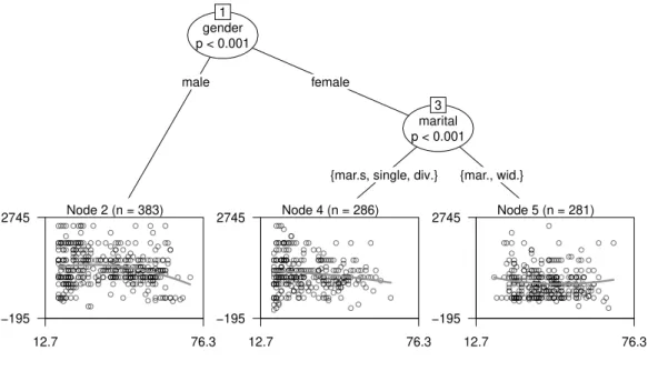
Figure 3: MOB: Assessing different relationships between age and requested in-come of unemployed respondents in Germany (SOEP 2008). The line pictures the estimated relationship in the current subsample and indi-cates the varying parameters according to groups related to age and marital status.
patterns of the association between the response variable and other covariates, that has been pre-specified in the parametric model. Therefore the end nodes in the model-based tree represent statistical models, such as linear models, and no longer mere values of the response variable. The execution of a split in the model-based tree then indicates a parameter instability in the original model, i.e. the postulated model is too simple to explain the data.
3.1. Basic principles of model-based recursive partitioning
As an instructive example for a partitioned model, Figure 3 shows the tree-structure for a sample of unemployed respondents from the SOEP study. The model of interest here is the relationship between the requested income, at which respondents would take on a new job, and the age. The functional form of this relationship is fixed to a quadratic polynomial as often found intuitive for models
relating age and income:
requested income =β0+β1·age +β2 ·age2+ε.
Additional covariates passed over to the algorithm are marital status, gender and nationality.
Beginning with the whole outlier adjusted sample of 959 unemployed respondents the model with the linear and quadratic term is fitted, where the estimated co-efficients βb0,βb1, and βb2 indicate parameter instability. The highest instability is
related to gender and thus a split in this variable is performed. While in the sample of the male respondents (node 2) no more instabilities are detected, the female subset is again divided into two subgroups with differing parameter esti-mates. The end node in the middle shows the result for married but separated, single or divorced women (node 4). The rightmost end node contains the linear model for married and widowed women (node 5). Interestingly, even the direction of the relationship changes from a parabola on the left, where men of higher age tend to request less income, to a slight u-shape on the right, where married or widowed women request more income in higher age. The attractive feature of im-plicit variable selection is also maintained in model-based recursive partitioning: the nationality does not occur in any split decision in this example.
node βb0 βb1 βb2
2 1014.5837 22.5446 -0.3618
4 1212.6621 -0.0236 -0.0871
5 1390.9708 -25.3983 0.2737
Table 1: Coefficients of the models in the end nodes.
In Table 1 the parameter estimates for the different groups – represented in the end nodes of the tree-structure – are displayed. The varying signs of the coefficients confirm what is illustrated in Figure 3: the inverse u-shape holds only for part of the sample and is reversed for other parts. Thus, the example illustrates that model-based recursive partitioning is indeed able to detect different functional
forms which might be masked when a single model is fit to the data.
The example also shows that, as opposed to classification and regression trees, the end nodes in model-based recursive partitioning do not contain values of a response variable, but represent a statistical model for each specific subpopulation. Between these groups the estimated parameters of the common underlying model vary significantly, but the postulated basic functional form (here polynomial) stated by the researcher is fixed. Within the subgroups no significant parameter instability is present.
Hence, the interpretation of a tree without any split is quite simple: there are no significant parameter instabilities found in any of the covariates handed over to the algorithm. If, however, a tree-structure is displayed, it reveals that the postulated model is not appropriate for describing the entire sample. The variation of the parameters highlights structural differences in the obtained subgroups, which can be easily interpreted by examining the estimates or the graphical output.
In the next section, important steps of the model-based partitioning algorithm are outlined. Then we take a closer look at the interpretation in social or behavioral sciences in Section 4.
3.2. Some technical details
The model-based recursive partitioning algorithm maintains the fundamental steps of the partitioning method reviewed in Section 2, but coherently extends them in the light of the model-based paradigm. According to this paradigm, the recur-sive process now estimates the basic statistical model beginning with all available observations. The result of this step is the estimated parameter vector from the optimization of the objective function, typically the (log-)likelihood. In almost the same manner as classification trees, the recursive process starts: instead of testing the association, now the parameter instability is assessed using so called general-ized M-fluctuation tests. If the data indicate parameter instability, the split of the parent node in two daughter nodes is executed. Relying on the data points in the new subgroups only, the algorithm again searches for parameter instability until no further significant instability is found, or another stopping criterion is fulfilled. This brief overview about the similarities and differences in the algorithms leaves some questions that have yet to be explained: Which models can be partitioned recursively? How can we assess parameter instability and where are the optimal
cutpoints in the covariates in model-based recursive partitioning? These questions are addressed in the next subsections, which are structured in the same way as Section 2.2.
3.2.1. The statistical model in the end nodes
The foundation of a general statistical framework for model-based recursive par-titioning by Zeileis et al. (2008) allows using a variety of underlying statistical models, such as linear and logistic regression models. The wide range of applica-tions emerges from the inclusion of several widely used test statistics in a unified approach (Zeileis 2005) called generalized M-fluctuation tests.
Technically, the generalized M-fluctuation test used for the split decisions relies on the objective function Ψ(.) of the parameter estimation, like least-squares and maximum-likelihood-estimation: b θ = arg max θ n X i=1 Ψ(yi, θ), (1)
where yi (i = 1, . . . , n) symbolizes the vector of all values of the dependent and independent variables in the postulated model for subject i, and θ represents the (potentially vector-valued) parameter. To keep the notation simple, here we use the full sample notation and do not distinguish whether the underlying obser-vations are the entire sample or a specific subgroup arising from the recursive application of the procedure.
The estimation process is based on the individual contributions of each subject i
to the score function
ψ(yi, θ) =
∂Ψ(yi, θ)
∂θ ,
as outlined below.
In addition to the model specification, the algorithm requires categorical or nu-meric covariates – denoted asZj (j = 1, . . . , l) – for potential splits in the model-based tree.
3.2.2. Selection of splitting variables
After the first step of the algorithm – fitting the underlying model for the whole
is performed. It is based on the statistical framework developed by Zeileis and Hornik (2007) to detect structural changes by fluctuation tests. In econometrics, these tests for structural changes are widely used to detect e.g. a drop in the expected value of a time series for a stock exchange due to an economic crisis. To detect a systematic change in the parameter over the range of a covariate Zj, the observations are ordered according to their values of Zj. Under the null hypothesis of parameter stability, no systematic structural change is present. The null hypothesis is rejected if one or more parameters of the postulated model change significantly over the ordering induced by the covariate Zj.
The construction of general test statistics relies on the partial derivatives of the objective function, e.g. of the log-likelihood. The contributions of each individual observationito the derivative of the objective function (i.e., to the score function) evaluated at the current parameter estimate, ψyi,θb
, are ordered with respect to the potential splitting variable Zj. The individual contributions ψyi,θb
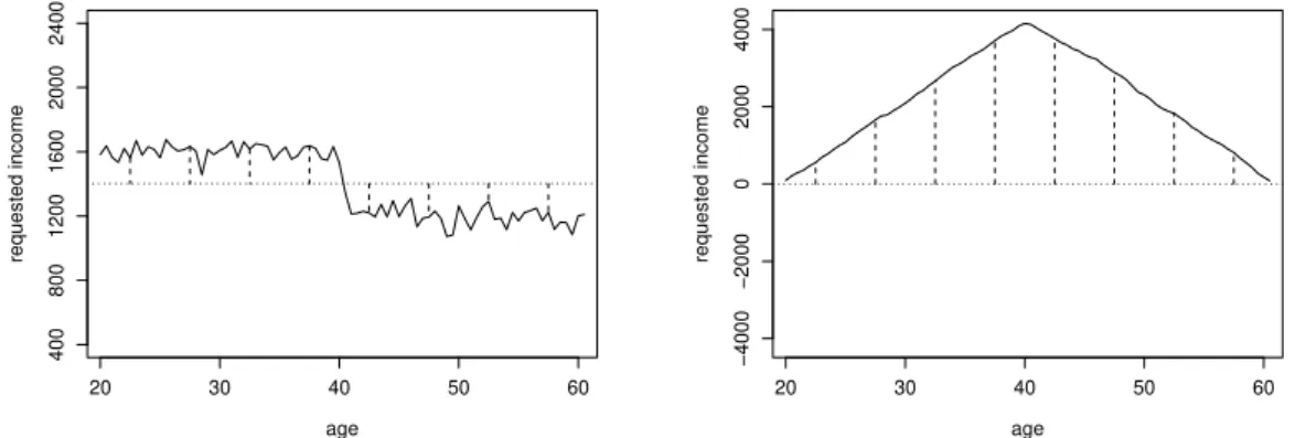
are depicted as vertical dashed lines for an instructive example in Figure 4 (left). Under the null hypothesis, the individual contributions ψyi,θb
should fluctuate randomly around the mean zero, whereas in Figure 4 (left) a clear structural change can be detected. To grasp this structural change statistically, we turn from the individual contributions to their cumulative sums in Figure 4 (right). Zeileis and Hornik (2007) proved the convergence of the cumulative sum process (also termed decorrelated empirical fluctuation process)
Wj(t) =Jb− 1 2n− 1 2 ⌊nt⌋ X i=1 ψyi,θb
against a k-dimensional Brownian bridge. The first part of the formula, Jb−12, denotes an estimator of the covariance Covψ(Y,bθ). The summation over all
⌊nt⌋ refers to the first n·t (with t ∈ [0; 1]) observations according to the order with respect to covariate Zj (for example the first 50%, where the ⌊.⌋ indicates that the integer part of n·t, i.e. the lower whole number, is used).
The instructive example in Figure 4 can be interpreted as the variation of income before and after the simulated threshold of 40 years. The path of the cumulative sum process increases until the age of 40 and decreases after that threshold, with a sharp peak at the change-point 40. The strength of this peak is used as a statistical
age requested income 20 30 40 50 60 400 800 1200 1600 2000 2400 age requested income 20 30 40 50 60 −4000 −2000 0 2000 4000
Figure 4: Structural change in the mean over age (artificial data). The left plot displays the mean income over all age groups (dotted line) and the indi-vidual deviations (dashed lines), the right the cumulated deviations over the variable age.
measure for the strength of the parameter instability.
The asymptotic properties of the cumulative sum process allows for the construc-tion of test statistics that are used for detecting the structural change. The test statistic for numeric variables is directly build from the empirical fluctuation pro-cessWj(t), while the test statistic for categorical variables takes into account that the categories and the observations within the category are not ordered. The result of Zeileis et al. (2008) also permits the computation of p-values and thus the statistical decision whether the parameters differ significantly from parameter stability. If parameter instability is detected, the algorithm selects the variable with the smallest p-value. Splitting continues until there is no further instability in any current node.
3.2.3. Selection of the cutpoint
In case of a splitting decision the cutpoint can be sought by a criterion that also includes the maximization of the objective function in the two potential subsam-ples. In the case of ordered or numeric covariates, these subsamples can easily be defined as L(ζ) ={i|zij ≤ζ} and R(ζ) ={i|zij > ζ} for a candidate cutpoint ζ and the component zij of zj.
The optimal cutpointζ⋆ is determined by maximizing X i∈L(ζ) Ψyi,θˆ(L) + X i∈R(ζ) Ψyi,θˆ(R) (2)
over all candidate cutpoints ζ. ˆθ(L) and ˆθ(R) are the estimated parameters in the
subsets. In case of unordered categorical covariates all potential binary partitions need to be evaluated and the partition with the highest criterion is chosen for the split (Zeileis et al. 2008).
Both parts of the binary split generate new parent nodes. Unless there is no further parameter instability found or another stopping criterion is satisfied (such as a minimum sample size in the current node) the algorithm continues searching for instability and splitting the current (sub-)data set in daughter nodes.
4. Potential in the social sciences
The application of model-based recursive partitioning offers new impulses for re-search in the social, educational and behavioral sciences. For the interpretation of model-based recursive partitioning, we would like to point out the connection to the principle of parsimony: following the fundamental research paradigm that theories developed in the social sciences should yield falsifiable hypotheses, the latter are translated into statistical models. The aim of model construction is thus to simplify the complex reality.
The decision on the complexity of the formulated model can be guided by “a
working rule known as Occam’s Razor whereby the simplest possible descriptions are to be used until they are proved to be inadequate” (Richardson 1958, p. 1247). This rule implies the objective of parsimonious model formulation: a model should be no more complex than necessary, but it also needs to be complex enough to describe the empirical data.
In the regression context usually the usage of sparse and simple models with few variables explaining the response are propagated (e.g. Gujarati 2003) – as long as important and relevant explanatory variables are not omitted. The strength of model-based recursive partitioning in this context lies in the power to let the data decide this question. Indeed, it offers the possibility to detect whether the sug-gested model is inadequate because relevant covariates are missing and it explicitly
selects these relevant covariates. If the algorithm executes at least one split, we obtain the statistical decision that the parameters are instable and the data are too heterogeneous to be explained by the postulated model. In this case, the pre-sumed functional form does not describe the entire sample in an appropriate way and thus subgroups have to be constructed.
Moreover, the tree-structured results provide information which subgroups differ in their association patterns. This information can either be integrated into a revision of the substantial theory and the formulation of a new parametric model, or it should be pointed out in the interpretation that the postulated model applies only to a limited scope of subjects.
Consequently, model-based recursive partitioning can identify different shapes of a parametric model stated by the researcher in different subgroups of the sam-ple. Model-based recursive partitioning offers nothing less than a synthesis of the theory-based and the data-driven approach that can be used for evaluating viola-tions of the ‘working rule’ Ockham’s Razor: if the method detects no instability of the model parameters, the postulated model is not rejected; but if the method does detect instability, the model is too simple.
5. Empirical example
To illustrate the potential of model-based recursive partitioning further, we turn to another example, based on an extension of the so called Mincer equation. In the seminal econometric work of Mincer (1974) the logarithmic income is described as a function of the variables years of schooling (time edu) and full-time experience (included in linear and squared terms, full ex, full ex2).
The Mincer equation owes its popularity to the straightforward interpretation of the coefficients as approximated rates of return from education (cf. Bj¨orklund and Kjellstr¨om 2002, for a critical discussion). We focus on the following extension of the Mincer equation that also includes a dummy variable for further education on the job (further edu):
ln (income) =β0+β1 time edu+β2 full ex+β3 full ex2+β4 further edu+ε
Here we restrict the observations from the SOEP study to over 6000 respondents in full-time employments who are not in vocational training and earn more than
500 Euros monthly.
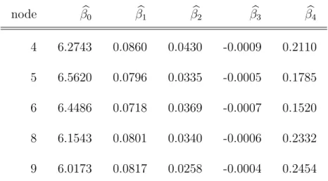
The examination of the Mincer equation, which is driven by the principle of parsi-mony, via model-based recursive partitioning is illustrated in Figure 5. The model formulation involves the effects (which are displayed as symbols in the end nodes) of years of schooling, further education and work experience in full-time jobs (linear and squared term) on the logarithmic gross income of fully employed respondents in Germany. Again, further potentially influencing variables are passed over to the algorithm, namely the location of the employer in east or west Germany, gender and the size of the company. The results show significantly different parameter estimates related to each of the additional covariates. These estimated coefficients of the Mincer equation are approximated rates of return e.g. from schooling. A closer look at the estimated parameters for the detected subgroups (Table 2) shows quite similar effects on the logarithmic income for some covariates from the orig-inal Mincer equation, such as the percentaged change for the time of education on earnings (βb1). However, the estimated coefficients for further education (βb4)
and the intercept (βb0) differ more strongly between the groups. In particular, the
effect of further education (βb4) is higher for employers in east as opposed to west Germany. node βb0 βb1 βb2 βb3 βb4 4 6.2743 0.0860 0.0430 -0.0009 0.2110 5 6.5620 0.0796 0.0335 -0.0005 0.1785 6 6.4486 0.0718 0.0369 -0.0007 0.1520 8 6.1543 0.0801 0.0340 -0.0006 0.2332 9 6.0173 0.0817 0.0258 -0.0004 0.2454
Table 2: Estimated coefficients of the models in the end nodes in Figure 5.
Our results match with current empirical social and economic research on het-erogenous effects of further education for men in Germany by Kuckulenz and Zwick (2005). Even though the estimated coefficients of the Mincer equation are
M O D E L-B AS E D R E C UR S IVE P AR T IT IO NI NG 19 location_emp p < 0.001 1 west east gender p < 0.001 2 male female size p < 0.001 3
{medium, small, large} {v. large, n.a.} Node 4 (n = 300) ● β0=6.3 β1 β2 β3 β4 −0.1 0.3 Node 5 (n = 2992) ● β0=6.6 β1 β2 β3 β4 −0.1 0.3 Node 6 (n = 1449) ● β0=6.4 β1 β2 β3 β4 −0.1 0.3 gender p < 0.001 7 male female Node 8 (n = 801) ● β0=6.2 β1 β2 β3 β4 −0.1 0.3 Node 9 (n = 550) ● β0=6 β1 β2 β3 β4 −0.1 0.3 ● Intercept years in school experience experience (sq.) further education re 5: M o d el-b as ed re cu rs iv e p ar tit io n in g of th e ex te n d ed M in ce r eq u at io n (S O E P 20 08 ). T h e sy m b ol s in th e en d n o d es ill u st ra te th e es tim at ed co effi cie n ts in th e su b gr ou p s re la te d to th e lo ca tio n of th e em p lo ye r, ge n d er an d siz e of th e co m p an y.
relatively stable in the subgroups, in this situation the original model is not in accordance with the principle of Ockham’s Razor because it is simpler than it should be. Our findings suggest the inclusion of theories explaining the different income levels in these subgroups, such as discrimination theories (e.g. Aigner and Cain 1977; Phelps 1972), and a more specific investigation of further education.
One reason for the violation of a joint model for all respondents may lie in the strong assumption of the Mincer equation that there is no relevant change in the economy under research. In the SOEP study, this assumption is clearly violated by the reunification of the eastern and western parts of Germany. As a consequence, we find a split according to the location of the employer in east and west Germany in Figure 5.
6. Software
The data analysis presented here uses the R system for statistical computing (R Development Core Team 2009), which is freely available under terms of the GNU
General Public Licence (GPL) from the Comprehensive R Archive Network at
http://CRAN.R-project.org/. Methods for classification, regression and
model-based trees are provided in the package party. The conditional inference
frame-work is implemented in the function ctree() (Hothorn et al. 2006b), while the
model-based recursive partitioning algorithm is available via the function mob()
(Zeileis et al. 2008). At the moment the algorithm can be applied to various types of generalized linear models, survival models or linear models. Moreover, the authors allow the users to build their own model classes and pass them on
to the existing mob() function. A vignette explaining the use of the software for
linear regression and logistic regression trees including the R-code is also avail-able (Zeileis, Hothorn, and Hornik 2010). Ongoing developments on the package
psychotreeexpand the application of the algorithm to psychometric models such as the Bradley-Terry model for detecting different preference structures (Strobl, Wickelmaier, and Zeileis 2010b) and the Rasch model for detecting different item difficulties among subgroups of respondents (Strobl, Kopf, and Zeileis 2010a).
7. Concluding remarks
Algorithmic procedures, such as classification and regression trees, have become popular and widely used tools in many scientific fields. Our aim here was to high-light that the recent development of model-based recursive partitioning allows to combine the power of these algorithmic methods with that of theory-based para-metric models by means of enhancing the purely data-driven approach towards a segmentation procedure for postulated models. Our presentation has highlighted the relation between this approach and the principle of parsimonious model con-struction. The tree-structured results allow straightforward interpretations of po-tential parameter instabilities that can be detected via empirical fluctuation tests. The detection of parameter instability leads to the interpretation that the statis-tical model under investigation cannot describe the whole sample appropriately, because relevant covariates have been omitted. Thus, model-based recursive par-titioning can be used as a diagnostic check for inadequately simple descriptions of the relationship between response and explanatory variables.
The application in social science research is eased by the freely accessible and well documented packages provided in the statistical software R.
8. Acknowledgements
Carolin Strobl is supported by grant STR1142/1-1 (“Methods to Account for Subject-Covariates in IRT-Models”) from the German Research Foundation (Deut-sche Forschungsgemeinschaft).
The authors would like to thank Achim Zeileis and Torsten Hothorn for their expert advice.
9. References
Aigner, Dennis J. and Glen G. Cain. 1977. “Statistical Theories of Discrimination
in Labor Markets.” Industrial and Labor Relations Review 30(2):175–187.
Berk, Richard A. 2006. “An Introduction to Ensemble Methods for Data Analysis.”
Sociological Methods & Research 34(3):263–295.
Bj¨orklund, Anders and Christian Kjellstr¨om. 2002. “Estimating the Return to
Investments in Education: How useful is the Standard Mincer Equation?”
Eco-nomics of Education Review 21(3):195–210.
Breiman, Leo, Jerome H. Friedman, Richard A. Olshen, and Charles J. Stone.
1984. Classification and Regression Trees. New York: Chapman and Hall.
Gujarati, Damodar N. 2003. Basic Econometrics, 4th ed. Boston: McGraw-Hill.
Hann¨over, Wolfgang, Matthias Richard, Nathan B. Hansen, Zoran Martinovich, and Hans Kordy. 2002. “A Classification Tree Model for Decision-Making in Clinical Practice: An Application Based on the Data of the German
Multi-center Study on Eating Disorders, Project TR-EAT.” Psychotherapy Research
12(4):445–461.
Hastie, Trevor, Robert Tibshirani, and Jerome H. Friedman. 2008. The Elements
of Statistical Learning. Data Mining, Inference and Prediction, 2nd ed. New York: Springer.
Hothorn, Torsten, Kurt Hornik, Mark van de Wiel, and Achim Zeileis. 2006a. “A
Lego System for Conditional Inference.” The American Statistician 60(3):257–
263.
Hothorn, Torsten, Kurt Hornik, and Achim Zeileis. 2006b. “Unbiased Recursive
Partitioning: A Conditional Inference Framework.” Journal of Computational
and Graphical Statistics 15(3):651–674.
Kitsantas, P., T. Moore, and D. Sly. 2007. “Using Classification Trees to Profile
Adolescent Smoking Behaviors.”Addictive Behaviors 32(1):9–23.
Kuckulenz, Anja and Thomas Zwick. 2005. “Heterogene Einkommenseffekte
Mincer, Jacob A. 1974. Schooling, Experience, and Earnings. New York: National Bureau of Economic Research.
Morgan, James N. and John A. Sonquist. 1963. “Problems in the Analysis of
Survey Data, and a Proposal.”Journal of the American Statistical Association
58(302):415–434.
Phelps, Edmund S. 1972. “The Statistical Theory of Racism and Sexism.” The
American Economic Review 62(4):659–661.
Quinlan, J. Ross. 1993. C4.5: Programms for Machine Learning. San Francisco:
Morgan Kaufmann Publishers Inc.
R Development Core Team. 2009. R: A Language and Environment for Statistical
Computing. R Foundation for Statistical Computing, Vienna, Austria.
Richardson, Lewis F. 1958. “Mathematics of War and Foreign Politics.” In New-man, James R., ed., “The World of Mathematics,” New York: Simon and Schus-ter.
Romualdi, Chiara, Stefano Campanaro, Davide Campagna, Barbara Celegato, Nicola Cannata, Stefano Toppo, Giorgio Valle, and Gerolamo Lanfranchi. 2003. “Pattern recognition in gene expression profiling using DNA array: a comparison
study of different statistical methods applied to cancer classification.” Human
Molecular Genetics 12(8):823–836.
Strasser, Helmut and Christian Weber. 1999. “On the Asymptotic Theory of
Permutation Statistics.”Mathematical Methods of Statistics 8:220–250.
Strobl, Carolin, Anne-Laure Boulesteix, and Thomas Augustin. 2007. “Unbiased Split Selection for Classification Trees based on the Gini Index.”Computational Statistics & Data Analysis 52(1):483–501.
Strobl, Carolin, Julia Kopf, and Achim Zeileis. 2010a. “Wissen Frauen weniger oder nur das Falsche? Ein statistisches Modell f¨ur unterschiedliche Aufgaben-Schwierigkeiten in Teilstichproben.” In Trepte, S. and M. Verbeet, eds., “Wis-senswelten des 21. Jahrhunderts - Erkenntnisse aus dem Studentenpisa-Test des SPIEGEL,” Wiesbaden: VS Verlag.
Strobl, Carolin, James Malley, and Gerhard Tutz. 2009. “An Introduction to Recursive Partitioning: Rationale, Application and Characteristics of
Classi-fication and Regression Trees, Bagging and Random Forests.” Psychological
Methods 14(4):323–348.
Strobl, Carolin, Florian Wickelmaier, and Achim Zeileis. 2010b. “Accounting for Individual Differences in Bradley-Terry Models by Means of Recursive Parti-tioning.”Journal of Educational and Behavioral Statistics In press.
Wagner, Gert G., Joachim R. Frick, and J¨urgen Schupp. 2007. “The German Socio-Economic Panel Study (SOEP) - Scope, Evolution and Enhancements.”
Schmollers Jahrbuch 127(1):139–169.
Zeileis, Achim. 2005. “A Unified Approach to Structural Change Tests Based on
ML Scores, F Statistics, and OLS Residuals.”Econometric Reviews 24(4):445–
466.
Zeileis, Achim and Kurt Hornik. 2007. “Generalized M-Fluctuation Tests for Pa-rameter Instability.”Statistica Neerlandica 61(4):488–508.
Zeileis, Achim, Torsten Hothorn, and Kurt Hornik. 2008. “Model-Based Recursive
Partitioning.”Journal of Computational and Graphical Statistics 17(2):492–514.
Zeileis, Achim, Torsten Hothorn, and Kurt Hornik. 2010. Party with the Mob:
Model-based Recursive Partitioning in R. R package version 0.9-9999.
Zhang, Heping, Chang-Yung Yu, Burton Singer, and Momiao Xiong. 2001. “Re-cursive partitioning for tumor classification with gene expression microarray
data.”Proceedings of the National Academy of Sciences of the United States of