Adaptive Preprocessing for Streaming Data
Indr ˙e ˇ
Zliobait ˙e, Bogdan Gabrys
F
Abstract—Many supervised learning approaches that adapt to changes in data distribution over time (e.g. concept drift) have been developed. The majority of them assume that data comes already pre-processed or that pre-processing is an integral part of a learning algorithm. In real application tasks data that comes from, e.g. sensor readings, is typically noisy, contains missing values, redundant features and very large part of model development efforts are devoted to data pre-processing. As data is evolving over time, learning models need to be able to adapt to changes automatically. From practical perspective automating a pre-dictor makes little sense if pre-processing requires manual adjustment over time. Nevertheless, adaptation of pre-processing has been largely overlooked in research. In this paper we introduce and address the problem of adaptive pre-processing. We analyze when and under what circumstances it is beneficial to handle adaptivity of pre-processing and adaptivity of the learning model separately. We present three scenarios where handling adaptive pre-processing separately benefits the final prediction accuracy and illustrate them using computational examples. As the result of our analysis we construct a prototype approach for combining adaptive pre-processing with adaptive predictor online. Our case study with real sensory data from a production process demon-strates that decoupling the adaptivity of pre-processing and the predictor contributes to improving the prediction accuracy. The developed refer-ence framework and our experimental findings are intended to serve as a starting point in systematic research of adaptive pre-processing mechanisms for adaptive learning with evolving data.
1
INTRODUCTION
A lot of research effort has been dedicated to making predictive models adapt to changing environment over time and lately the attention to such learning scenarios has been rapidly increasing [1]–[6]. As data evolves over time, predictors need to have opportunities to update or retrain themselves, otherwise they will become less ac-curate. The majority of adaptive predictors assume that data comes already pre-processed or that pre-processing is an integral part of a learning algorithm.
In real applications pre-processing is a very impor-tant step of data mining process, as real data often comes from complex environments and is often noisy and redundant. Data mining practitioners claim (e.g. [7]) that data preparation takes 80 − 90% of a data mining project time, which means that modeling can take as little as 10%. In contrast, in adaptive learning • I. ˇZliobait˙e and B. Gabrys are with Smart Technology Research Centre, School of Design, Engineering and Computing, Bournemouth University, Poole House, Talbot Campus, Fern Barrow, Poole, Dorset, BH12 5BB, UK. E-mail:{izliobaite,bgabrys}@bournemouth.ac.uk
research publications data pre-processing is surprisingly understudied or gets low priority in comparison to de-signing adaptive predictors. As changes in data happen, adapting only predictor may not be enough to maintain a good accuracy over time, as we will see from our examples and the case study with a real production data. Moreover, if we do not adapt pre-processing, our adaptive predictor may fail and in some cases give even worse results than non-adaptive predictors. Finally, designing automatically adaptive predictors makes little sense from practical perspective if pre-processing needs to be adjusted manually as time passes.
The most obvious approach to automate pre-processing in adaptive learning is to keep pre-pre-processing tied with adaptive predictors, which can be done in two cases. The first option is to reserve a validation set at the beginning, optimize the pre-processing parameters on that validation set and keep the pre-processing fixed for the lifetime of the model. Only the predictor itself would adapt over time. The problem with this approach is that the system may easily fail to notice changes that happen in the raw data, and thus fail to adapt. Consider a chemical production process where input data comes from sensors and the goal is to predict the output quality. When a sensor gets old its readings may become noisy and non informative, thus the reading of this sensor may not be selected during the feature selection step. Suppose after some time this old sensor gets replaced, and the readings become more relevant to prediction. However, as we fixed the selection of features at the beginning, we no longer have this sensor in our feature space thus we lose an opportunity to adapt and improve our predictions.
The second option is to redo all pre-processing from scratch every time the predictor is retrained. This ap-proach requires the retraining of pre-processing and a predictor to be synchronized. That may be problematic if, for instance, preparing an accurate pre-processing requires more data than training a predictor. That may be even infeasible in cases when an incrementally adaptive predictor is used, which updates its parameters with every new instance. Last but not least, redoing the pre-processing on every data chunk may introduce unneces-sary computational costs.
We investigate how to integrate adaptivity of pre-processing with adaptivity of a predictor in evolving
streaming data. We demonstrate that it may be bene-ficial to handle adaptive pre-processing and adaptive predictors separately. Our study makes a threefold con-tribution. Firstly, we formulate the concept of adaptive pre-processing that has been overlooked in developing adaptive learning models. Pre-processing is an essential step in developing real world applications and it also needs to be adaptive. This paper is the first attempt to provide a systematic view towards pre-processing in adaptive learning. Secondly, we develop a reference framework for adaptive pre-processing that connects online learning scenarios with potential benefits from adaptive processing and approaches to make pre-processing adaptive. Within this framework tailored adaptive pre-processing approaches can be designed. A prototype adaptive pre-processing approach, that we develop following the reference framework and evaluate with a real sensor data from production process, is the third contribution.
The remainder of the paper is organized as follows. Section 2 presents our reference framework for adaptive pre-processing. In Section 3 we analyze three scenarios of adaptive pre-processing resulting from our framework employing synthetic toy examples. Section 4 introduces a prototype system that is able to perform adaptive pre-processing in separation from adaptive predictor. We experimentally evaluate our prototype in Section 5. Finally, Section 6 discusses related work and Section 7 concludes the study.
2
REFERENCE FRAMEWORK FOR ADAPTIVE
PRE-PROCESSING
To provide a motivation for decoupling adaptive pre-diction and adaptive pre-processing, we examine what types of adaptive learning are available and in what ways they may interact with pre-processing. By adap-tive processing we mean that the adaptivity of pre-processing is not tied to the adaptivity of the learn-ing model. Our reference framework for adaptive pre-processing includes four main elements: (1) categoriza-tion of pre-processing techniques, (2) characterizacategoriza-tion of changing environment, (3) characterization of adaptive learning and (4) the scenarios for interaction between adaptive predictors and adaptive pre-processing in a changing environment, which is the connecting element. We first define the setting of the study and then introduce the elements of our reference framework.
2.1 Setting
This study of adaptive pre-processing is restricted to supervised learning scenarios. LetX be an instance ind -dimensional space and letybe its label (target variable). The goal in traditional supervised learning is to learn a model y =L(X) and use it for predicting the labels of unseen data.
In adaptive learning the data arriving over time forms a data stream X1, X2, . . . , Xt, . . .. We can use L for
all predictions. Alternatively, when the true labels ar-rive shortly after we cast the prediction, we have an opportunity to regularly update the model using the new data. The model for time t can be represented as
Lt=f(Lt−1, Xt−1, yt−1). Note that an update is optional, i.e. it may be that Lt=Lt−1 or Lt6=Lt−1.
Pre-processing maps data into a format that can be more effectively used in training and applying a predic-tor. LetXrepresent our raw data. The preprocessing step makes a mapping X0 =G(X). Then the prediction step makes a mappingy=L(X0). Examples of pre-processing include: outlier detection and removal, replacing missing values, data normalization, data rotation, feature selec-tion or/and extracselec-tion/generaselec-tion. A pre-processor and a predictor will be referred to as alearning component.
A predictor L maps data from multi-dimensional in-put to one-dimensional outin-put (target variable). A pre-processor G maps data from a multidimensional input to a multidimensional output (e.g. using dimensional-ity reduction techniques, such as Principal Component Analysis (PCA) [8]). For example, a Naive Bayes clas-sifier can serve as a prediction function, and PCA can serve as a pre-processing function.
2.2 Types of pre-processing [Element (1)]
Pre-processing actions can be characterized by several properties which determine the feasibility and the need for adaptive pre-processing.
Feedback. A pre-processorG may need to be learned on a training dataset so that it could be applied to unseen data. Learning a pre-processor G can be super-vised,unsupervisedorindependentof the data. Supervised learning of the pre-processor means that the original data X with its true labels y are used in the learning process, e.g. feature selection based on correlations of the input variables with the label. Unsupervised learning means that only the original dataXis used for learning the pre-processor, e.g. feature extraction using principal component analysis. Independent learning means that only the parameters of the data, but not the data itself are fixed in the learning process, e.g. random projection for feature extraction [9].
Operation. A pre-processor can operate in an eager
way meaning that the parameters of G are fixed in the process of learning and G can be applied to new data, orlazyway, meaning that the parameters are determined from the actual incoming new data. For instance, feature extraction using principal component analysis [8] is an eager pre-processing procedure, a rotation matrix can be learned on training data and fixed. On the other hand, handling missing values can be seen as a lazy procedure, where, for instance, a moving average of recent values is used to impute the missing value.
Validation. Validation of an eager pre-processor can be organized in adirectorindirectway. Direct validation optimizes some criterion in the process of pre-processing itself, e.g. in feature selection based on correlation with
preserving transformation input
variables
result of pre-processing
Fig. 1. Variable transformation.
the target variable, maximization of the correlation is used as the chosen criterion. Indirect validation means that a feedback from the actual predictor is needed, for instance, random feature subsets are formed and the subset that leads to the best final prediction accuracy is selected. If the predictor is itself adaptive, the feedback over time may be noisy as the evaluation mapping Lis evolving over time.
Feature transformation.A pre-processing procedureG
may transform or preserve the original variables. For in-stance, data rotation using PCA would transform, while feature selection would preserve the original variables, as illustrated in Figure 1.
Coverage. Preprocessing procedures can be global in a sense that the same treatment is applied to every instance, orlocalin a sense that every instance is treated individually. Variable normalization to zero mean and unit variance is an example of global preprocessing, while imputation of missing values is an example of local pre-processing. Missing values are imputed not for every instance, but only for the instances where the values are missing.
Table 1 characterizes several examples of pre-processing techniques in terms of the discussed prop-erties. A reader is referred to e.g. [8] for more details on pre-processing techniques.
Note that in case of instance based pre-processing every instance is processed individually, thus there is no need for centralized adaptivity of the pre-processor. Thus, our further analysis focuses on trainable pre-processing procedure, which use eagerlearning and are of global applicability, as in such a case we learn global models, which may need to be adapted later.
2.3 Making pre-processing adaptive
Pre-processing does not operate in isolation as it is a part of adaptive system. As the system is adapting, models that are used by the system change over time, in line with changes in data over time. The objective of an adaptive system is to adapt to changes in data. However, having more than one adaptive component in the system introduces an extra challenge, since in addition to adapting to changes in data each component may need to adapt to changes in other components.
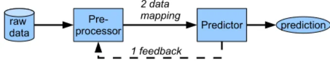
A pre-processing component in adaptive prediction system has two main connections, as illustrated in Figure 2. First, the pre-processor may need feedback from the predictor to decide upon adapting and/ or re-training itself. Second, the pre-processor produces a
Pre-processor Predictor 2 data mapping 1 feedback raw data prediction
Fig. 2. Pre-processing and prediction in adaptive system.
mapping that transforms the raw data, which is then used by the predictor. Thus, when deciding whether to decouple adaptivity of pre-processing and adaptivity of the predictor the consistency of the two links needs to be assessed and handled, i.e.:
1) consistency of feedback over time, and 2) consistency of feature mapping over time.
Handling the first issue is essential, since adaptivity of the predictor may contaminate the feedback, based on which the pre-processor decides whether and when to adapt, and this feedback is needed for updating of the pre-processor. As mentioned earlier, learning of the pre-processor may be supervised, unsupervised or inde-pendent from the actual data. Validation of the learning can directly optimize a chosen criterion, or indirectly use the prediction error for validation. Learning that is independent from feedback (such as random projection method [9]) is expected to be consistent and robust to evolution of the predictor, thus changes in the link #1
would not cause problems to the system.
Unsupervised learning (such as PCA [8]) is expected to be consistent and robust if it is learned using a direct val-idation procedure and parameters are optimized directly. In such cases evolution of the predictor would not cause any problems for the pre-processor, as the link#1 will not be active. However, if an unsupervised learning of the pre-processor uses a predictor for indirect validation (e.g. to decide how many principal components of PCA to keep several options are tested with the actual predic-tor and the option that minimizes the validation error is selected), then due to the link #1 the performance of the pre-processor may be affected by evolution of the predictor and the pre-processing procedure may need to be adapted to that. The same effect of an indirect validation is expected for supervised learning of a pre-processor.
The link #2 is essential for assessing consistency of feature mapping over time, since the predictor takes as an input the output of the pre-processor. If the mapping of that input changes, the predictor may be forced to be retrained and that restricts possibilities for decoupling of the two components.
2.4 Changing environment [Element (2)]
We are considering adaptive learning mechanisms for streaming data where changes in data distributions are expected to happen over time. These changes may be of different types and depending on the type of changes different adaptivity may be necessary in pre-processing
TABLE 1
Examples of pre-processing techniques and their properties.
Feedback Operation Validation Feature transformation Coverage
Feature selection using correlation supervised eager direct preserve global
Feature extraction using PCA unsupervised eager direct/indirect transform global
Feature extraction using random projection independent eager indirect transform global
Moving average imputation of missing values unsupervised lazy direct preserve local
and prediction. In addition, changes in the data distri-bution can affect the whole feature space or they can be
localaffecting only particular features or only particular ranges of particular features.
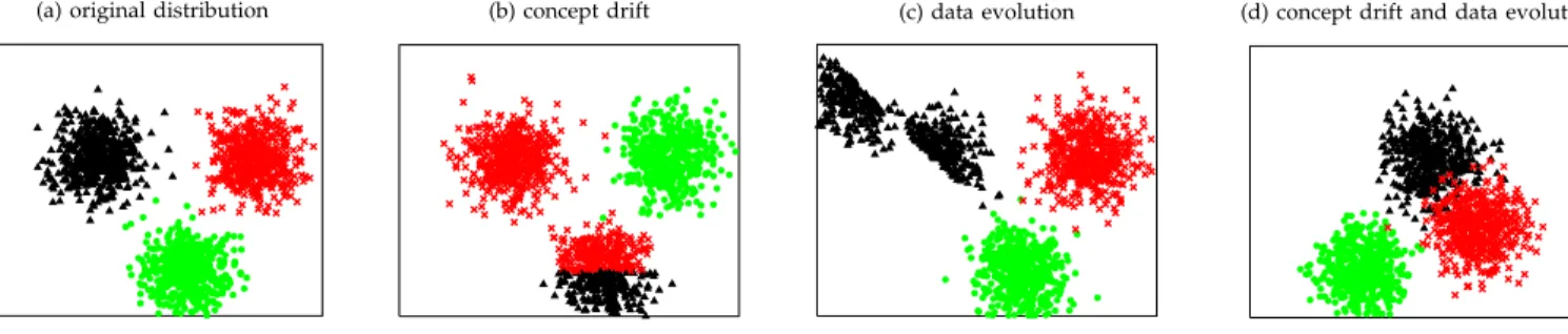
Suppose data comes from a distributionp(X, y), which may change over time. Changes in data distribution can be described as concept drift, data evolution or both. Figure 3 (a-d) presents a toy example that illustrates the main types of changes. The original data (a) forms three classes. A (real) concept drift (b) does not affect the data distribution p(X), only the joint distribution p(X, y) changes. Data evolution (c) changes the input data distribution p(X), at the same time the relation between the input variables and the targets stays the same. In reality a concept drift and data evolution often happen together as illustrated in (d).
In the literature [10] (real) concept drift typically refers to changing relation between the input data and the tar-get variable (b). Since there is no data evolution, only the labels change, such a drift typically would not require adaptation of the pre-processing, adapting the predictor would be sufficient. Data evolution, also referred to as virtual drift, is likely to require adaptation of the pre-processor since the input data representation changes (c). This drift in isolation, however, may not require adaptation of the predictor, if the relation between the concepts (classes) does not change. In such cases it may be sufficient to adjust the pre-processing so that new data is repositioned to appear where the old data previously was appearing (as we will illustrate in our analysis in Section 3). In cases where both types of drift take place (d) we may or may not need to adapt the pre-processing, but typically we would need to adapt the predictor. As we will demonstrate in our analysis in Section 3, changes in data (d) may happen in such a way that both adaptations are required, but it may be optimal to execute those adaptations asynchronously, i.e. at different times after the change.
So far we have discussed the situations where changes happen in such a way that the data ‘moves’ and new con-ceptsreplacethe previous ones. Data may also evolve to cover new regions in the instance space or represent new concepts that have not been seen before. For example, appearance of a new class is referred to as concept evo-lution [11] in the literature. As time passes, we observe new data that complements the previously observed data and we may need additional pre-processing and prediction mechanisms, which also requires adaptive learning.
2.5 Adaptive learning [Element (3)]
For presenting meaningful scenarios of adaptive pre-processing we need to characterize adaptive learning approaches. These approaches describe mechanisms be-hind adaptive predictors, but they can be directly trans-lated for application to adaptive pre-processors.
Adaptation of predictive models can beincrementalor use replacement, as presented in Figure 4. Incremental approaches incorporate new data into existing models, while replacement approaches discard the old model and learn a new one from scratch on the new data.
Incremental learning approaches can increment at an instance level, at batch level or at an ensemble level. At an instance level the parameters of the model are updated with the information extracted from one incom-ing data point. At a batch level the parameters of the model can only be updated after a number of incoming data points have been seen. For instance, more than one new data point may be needed for estimating the current accuracy. This approach is considered to be incremental, since the old model is not discarded to be learned from scratch, but only updated.
Incremental learning can happen at an ensemble level, where a new model is built with the new data chunk, while the old models stay the same. In this case individ-ual models are not updated incrementally. Adaptivity is achieved by manipulating the weights of individual models to output the final prediction.
Replacementapproaches can be described as full or par-tial. Full replacement means that given a new chunk of data the pre-processor and the predictor are learned from scratch. Partial replacement means that some parts of the model are fully replaced. Consider the Naive Bayes (NB) classifier as an example. NB makes an assumption that the input features are independent from each other. Thus one feature can be completely replaced, with new
ADAPTIVE LEARNING INCREMENTAL update model INSTANCE update with every instance BATCH update in batches ENSEMBLE add/ remove classifiers REPLACEMENT replace model FULL replace all PARTIAL replace part of the model
(a) original distribution (b) concept drift (c) data evolution (d) concept drift and data evolution
Fig. 3. Illustration of changes in data distribution.
probability counts (obtained after a new pre-processing), while probability counts for the other features can be preserved. Such approach can be beneficial if the drift happens locally not affecting the whole feature space.
2.6 Adaptive pre-processing scenarios [Element (4)]
The last element of the reference framework character-izes the interaction between pre-processing and predict-ing in adaptive learnpredict-ing. At any given point in time there may be a need to adapt the pre-processor, the predictor, adapt both or none. Four scenarios of interaction that may occur in a streaming data over time are described in Table 2.
TABLE 2
Scenarios of interaction between pre-processing and prediction in adaptive learning.
S0 S1 S2 S3
Need to adapt pre-processing no no yes yes
Need to adapt the predictor no yes no yes
Suppose both the pre-processor and the predictor adapt in the replacement mode. In Scenario S1 there is
no need to adapt the pre-processor, but the predictor needs to be adapted. Such situation may occur when the input data does not change, but the relation between the input and the target variables changes (Figure 3b concept drift). For example, a reader is reading news online, he has been interested in real estate prices, but suddenly his interest changes and real estate articles are no longer relevant. This scenario is valid if unsupervised pre-processing is used.
In Scenario S3 there is a need to adapt both the
pre-processor and the predictor. This may occur when the in-put data distribution changes (Figure 3c data evolution). For instance, in streaming news example new words may appear. As a result a new feature extraction needs to be performed and the predictor retrained correspondingly. In Scenario S2 there is no need to adapt the
predic-tor, but the pre-processor needs to be adapted. Such situation may occur when the distribution of data does not change, but the noise on data changes. It also may occur when the concepts move, but the relation between concepts does not change (a variant of (d) in Figure 3). For example, as a sensor wears off, new types of outliers
appear (or missing values appear where they were not present before). As a result we may want to change a mechanism for outlier detection. But the cleaned in-stances will represent the same concept. Therefore, the same predictor can be applied.
Finally, in scenarioS0the data is stationary and there
is no need to adapt.
When the pre-processor and the predictor adapt in an incremental mode both models are updated at every time step, thus we always encounter scenario S3. An
interesting situation may occur if one of the components adapts in an incremental mode, while the other adapts via replacement. It is not expected to be that challenging if the pre-processing adapts in an incremental mode, but the predictor adapts via retraining, as in such a case the predictor would treat incremental changes in the pre-processing output as it would treat raw changing data. This setting would present scenarios S2 or S3 where
the pre-processor always adapts. On the other hand, the situation where pre-processor adapts via replacement and the predictor adapts incrementally is potentially more challenging, since the predictor would be exposed to a sudden concept drift induced by replacing the pre-processor, that is not necessarily present in the real data. Thus the systems in such situations would require well thought through design to exploit the benefits of adaptive pre-processing. This setting would result in scenarios S1 or S2, where the predictor always adapts.
We will investigate this situation as one of the analytical experiments in the next section.
Ideally an adaptive learning system should be able to handle all the scenarios. Current approaches typically can handle only S0 and S1. Even in those cases there
is a constant pressure on developing better performing adaptive methods. With a little modification (online pre-processing) some of the systems would also be able to handleS3. However, they would be able to handle either
S1 or S3, but not both. We will explore this situation
experimentally in our next section. We are not aware of approaches that could handle or would considerS2, and
we will also explore this scenario in the next section.
3
A
NALYSIS OF DECOUPLING ADAPTIVE PRE-PROCESSORS AND ADAPTIVE PREDICTORS
Now as we described the elements of the adaptive pre-processing framework, let us take a closer look at
situ-ations in which decoupling adaptivity of pre-processing and adaptivity of the predictor in the same system makes sense. We investigate the situations when pre-processing needs to be adapted, but the predictor does not need to be adapted, as represented by the scenario S2, and
the situations where there is a need for adaptivity, but not at the same time in both components, as a part of the scenario S3. The following situations may require
decoupled adaptivity.
Situation A: the two components require different amount of data for training - this happens within Scenario S3. For instance, a Naive Bayes can be
trained from a small number of data points, while to execute PCA we will need more data.
Situation B: changes in data do not change the relation between the concepts (classes) in data (e.g. change in noise of data or data evolution without change in the decision boundary), Scenario S2.
Situation C: in the incremental learning scenario (no re-access to the historical data) changes in pre-processing need to be introduced while the incre-mental updates to the predictor are continuously executed, Scenario S3 .
Next we present and analyze three classification exam-ples that correspond to each situation. The goal of our simulation is to demonstrate in what situations decou-pling of adaptivity of the pre-processor and the predictor may be beneficial to the prediction accuracy. Table 3 summarizes the settings of our analytical experiments.
We analyze the three situations with examples of syn-thetic data. We use different pre-processing techniques to demonstrate the scope and applicability of adaptive pre-processing and we use the Naive Bayes classifier as the predictor. Note that our focus is to demonstrate the situ-ations, we are not designing algorithms for adaptive pre-processing, thus to inspect the effects of pre-processing alternatives these simulations use a simplifying assump-tion that the time of a change is known.
3.1 Situation A: different amount of data is required
The first situation illustrates the case when different amount of data is required to train the pre-processor and to train the predictor. Consider the following example of a binary classification task. Data points lie in 20 -dimensional space, where the first three dimensions are relevant for classification. The classes are distributed as Xi∼ N(mi, C), where iis the class number andC20×20
is the covariance matrix. Details of the distribution are given in Appendix A.
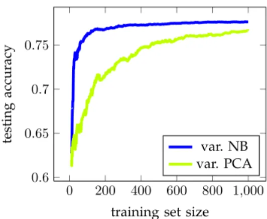
Experiment 1.Our first experiment with this scenario demonstrates that the pre-processor and the predictor require different amount of data for training in a static case. Let us use PCA as pre-processing technique and Naive Bayes as the predictor. We fix the number of extracted principal components to four. For training the pre-processor, training the predictor and testing the performance we generate three independent datasets of
0 200 400 600 800 1,000
0.6 0.65 0.7 0.75
training set size
testing
accuracy
var. NB var. PCA
Fig. 5. Effect of training set size to accuracy.
sizes nP CA, nN B and ntest respectively, that follow the same distribution N. We fix ntest=10 000, and run two cases: (1) nN B=10 000 is fixed, while nP CA varies in
[4. . .1000]; (2) nP CA=10 000 is fixed, while nN B varies in[4. . .1000].
Figure 5 plots the dependence of the prediction ac-curacy as a function of training set size averaged over 10 runs. The PCA line shows what happens if we in-accurately learn the pre-processor due to lack of data, and NB shows the same for the predictor. The results suggest that in this situation more data is required to train an accurate pre-processor than predictor. That is explainable by the fact that the pre-processor needs to be trained on much larger dimensional data (p = 20) than the predictor (p= 4), thus may require more data for accurate training. Therefore, in online learning we may need to adapt the pre-processor and the predictor at different times after change happens to achieve an optimal result.
Experiment 2.Let us now consider what happens if a change in data distribution happens over time. Let our data come in a stream from a distributionXi∼ N(mi, C) until timet, and then start to come from a distribution Xi∼ NII(m0i, C). The details of the two distributions are given in Appendix A. Our second experiment compares the accuracies of three learning systems assuming that the point of change is known.
In the first system (‘old-old’) both the preprocessor and the predictor are trained on the data (10 000 in-stances) distributed asN. The second system (‘old-new’) uses the old pre-processor, but retrains the predictor with the new data that comes after the change, assuming that the change point is known. The third system (‘new-new’) retrains both the predictor and the pre-processor on the same new data that comes after the change.
For every point in time we generate an independent test set of 10 000 instances following the distributionNII defined earlier and test the performance of the three systems. Figure 6 presents the results averaged over 10 runs. The ‘old-old’ plot represents a fixed model that does not get updated over time, therefore, as the data distribution remains fixed after the drift, the accuracy of
TABLE 3
Summary of the experimental setting.
Feedback Features Adapt pre-pro Adapt predictor
Situation A unsupervised transform replace/increment replace/increment Situation B unsupervised preserve replace/increment replace/increment
Situation C supervised preserve replace increment
0 50 100 150 200
0.7 0.8 0.9
time after change
testing
accuracy
old-old old-new new-new
Fig. 6. Effect of re-training to accuracy.
the performance stays at the same level. We can see from the figure that there is a time period where it is beneficial to retrain only the predictor, but not the pre-processor (‘old-new’). Later it becomes beneficial to retrain both.
These experiments illustrate that decoupling adap-tivity of pre-processor and predictor may be beneficial in cases when the two components require different amounts of data for learning an accurate model. A ques-tion for further research is how to determine online what should be the optimal training history for each adaptive component. In the last part of this paper we will develop and demonstrate a simple prototype technique based on cross validation that sets different training windows for pre-processing and prediction when learning from real data stream where different types of changes can happen.
3.2 Situation B: data evolution with no effect on the decision boundary
The previous experiment illustrated the situation where pre-processing and predictor were adapting at different phases. The next experiment presents a surprising case where we need to adapt only the pre-processor, while the predictor stays untouched. In such a case retraining the predictor not only unnecessarily increases computational costs, but also may harm the prediction accuracy.
Such a situation may occur when the data evolves in such a way that the relations between the input variables and the target variable is not affected (e.g., the type of noise or missing values on the input variables change). In such a case there may be no need to change the predictor, but the pre-processor would need to adapt. The next experiment demonstrates how withholding
from retraining the predictor may be beneficial to the final accuracy.
This experiment presents a classification problem where given a 10-dimensional input vector the goal is to predict a target, that is a linear combination of noisy input variables. We generate a data stream where a change in data distribution happens at time t =10 000 and report the testing errors (the root mean square error) from the change point onwards. The details of the two distributions are given in Appendix A. We assume again that the change point is known. Change happens only in one of the dimensions and we assume that we know in which. Knowing that, we retrain the pre-processor only for that particular variable where the change happens. Such a situation may occur in chemical production pro-cess, e.g. when one sensor is replaced. We know when it was replaced and which variables were affected, but we don’t know what the effect was.
We use normalization (subtract the mean, divide by the standard deviation) as the pre-processor and the Naive Bayes classifier as the predictor. We compare the performance of four systems: ‘old-old’, ‘old-new’, ‘new-old’ and ‘new-new’. The baseline ‘old-‘new-old’ does not retrain either the pre-processing or the predictor after the change. The tied system ‘new-new’ retrains both components on the same training sets. In every step it uses all the data after the change until the current time for retraining. ‘old-new’ does not retrain the pre-processor, but retrains the predictor. Finally, ‘new-old’ is the system of interest, which retrains the pre-processing, but leaves the predictor untouched.
Figure 7 presents the results averaged over 10 runs. It can be clearly seen that right after the change ‘new-new’ (and ‘old-‘new-new’) is suboptimal, because there is too little new data to train an accurate model. Gradually it starts to improve, but our system of interest ‘new-old’ performs better. The old predictor has been trained on a large old dataset (10 000), it is sufficient to make a tiny adjustment to the pre-processing and the old model becomes suitable for the new situation. We can observe a slight upward inclination at the beginning in the error of ‘new-old’, which is the price paid for estimating a new pre-processor from a small amount of new data. The performance of ‘new-old’ is superior, as, in contrast to Situation 1, in this case training an accurate pre-processor requires much less data than to accurately retrain the10-dimensional predictor.
0 100 200 300 0.9
0.92 0.94
time after change
testing
accuracy
old-old new-old new-new(=old-new)
Fig. 7. Benefits of no retraining.
3.3 Situation C: incremental and replacing adaptiv-ity together
The two situations that we discussed concerned the learning scenarios where adaptivity is achieved by re-placing old models. This final section discusses the situation when at least one component adapts in an incremental manner. Recall that incremental adaptivity means that a model is not replaced, but the parameters of the existing model are updated with the latest incoming data. Thus in the replacement mode the model at time t is
Lt=f[(Xi, yi),(Xi+1, yi+1), . . . ,(Xt−1, yt−1)],
while in the incremental mode the model can be repre-sented as
Lt=f[Lt−1,(Xt−1, yt−1)].
Four combinations of interactions between pre-processing and prediction in terms of adaptivity mode are possible as specified in Table 4. We already analyzed examples where both components are adapted immedi-ately by replacement. When both components adapt in the incremental mode, adaptivity is achieved in small steps and there is not much room for decoupling. The case when the pre-processor adapts in the incremental mode is not that challenging either as here pre-processor acts as a filter and the predictor can provide all the adaptivity that is required.
TABLE 4
Combinations of retraining and incremental adaptivity.
adaptivity of Sit. A,B X
pre-processing replace increment replace increment
predictor replace replace increment increment
Our main interest in this setting is to investigate the case when the pre-processor adapts immediately and the following predictor adapts in the incremental mode. This case is not trivial, as discussed in Section 2.3, since in addition to adapting to changes in data, adapting to changes in the other component may be necessary. Due to replacement of pre-processing, suddenly we may have completely new mapping of data. The incremental
predictor may perceive the replacement of pre-processor as a sudden change that may not necessarily be optimal at all times. The question for research is what to do in such a case. One could start new predictor from scratch or keep the old model, or maybe switch the predictor to the replacement mode. Our next experiment illustrates the situation.
To analyze the impact of changes in the feature space to adaptivity of the predictor we return to classification example and perform the following experiment. Suppose our data lies in the 8-dimensional input space with an associated binary classification task. The input variables are noisy, but the level of noise on each feature varies. We use feature selection as the pre-processing step and to simplify the setting we do feature selection based on our knowledge of the underlying data model. We use the Naive Bayes and the incremental predictor.
Suppose a change in data distribution happens at time t. At that point the level of noise on certain features changes and, as a result, the relevance of certain fea-tures to the classification problem changes. Thus the pre-processing needs to change in order to maintain the optimal accuracy of the final prediction. The main restriction comes from the incremental learning setting since the historical data is not stored in memory. There-fore we cannot go back and retrain our classifier with the historical data while applying the newly selected features. We have three main options how to proceed with training:
1) (old-old) We can continue incrementally updating the existing classifier; however, the current feature subset will remain suboptimal.
2) (new-old) We can continue updating the same model but use the newly selected features. Intu-itively, the applicability of this strategy will depend on how many of the old features stay in place and ability of the prediction model to operate in changing input space.
3) (new-new) We can start training a new model with new features from scratch.
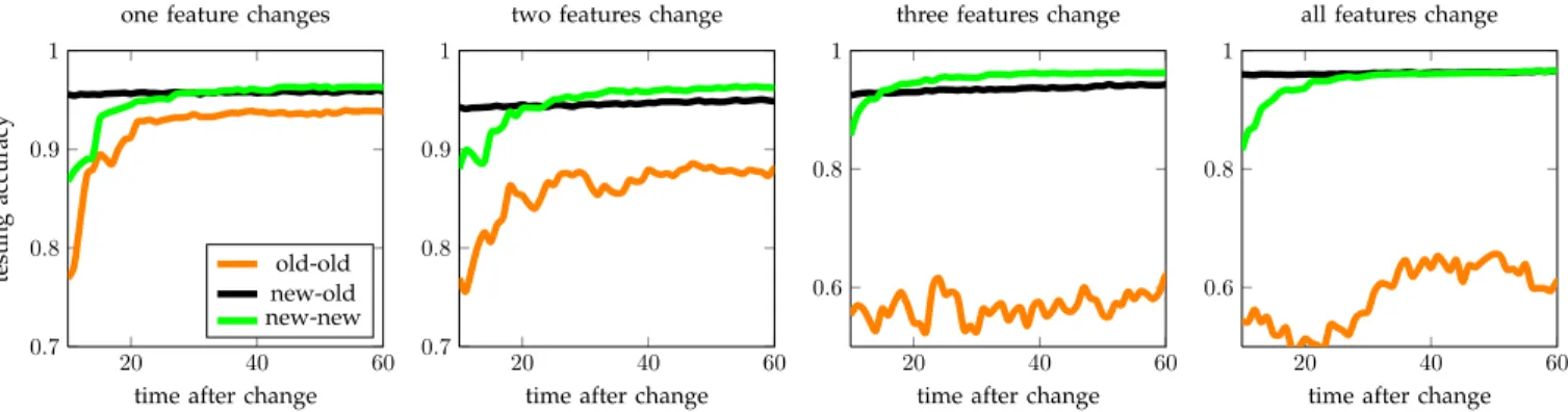
Our experiments compare the accuracies of the three strategies. The details of the data distributions are pre-sented in Appendix A. In the pre-processing step we select four features that later are used for training a classifier. Figure 8 presents the accuracies when one, two or three features are replaced as a result of the change in data distributions.
We see that in all situations right after the change ’new-old’ approach, which updates the old classifier with newly selected features performs better than the one that uses the old features (’old-old’) and the one that starts training from scratch (’new-new’). As it can be expected, the benefits to the accuracy are more substantial when fewer features get affected by the change. The results show that even under incremental learning (where we have no access to historical data) there is a room for decoupling adaptivity of pre-processing and adaptivity of the predictor that may
20 40 60 0.7
0.8 0.9 1
time after change
testing
accuracy
one feature changes
old-old new-old new-new 20 40 60 0.7 0.8 0.9 1
time after change two features change
20 40 60
0.6 0.8 1
time after change three features change
20 40 60
0.6 0.8 1
time after change all features change
Fig. 8. Incremental learning with changing relevance of features.
benefit the final accuracy.
To summarize, we identified the gap in existing adap-tive learning approaches, as they do not consider pre-processing to be adaptive on its own. We systemati-cally analyzed possibilities and challenges to integrate adaptive pre-processing and adaptive predictor into one system. We identified and experimentally illustrated three situations in which decoupling the two adaptive components may be beneficial to the final accuracy. This study opens a list of important research questions to be answered in order to be able to apply adaptive pre-processing along with adaptive learning. The following problems for further research can be identified.
• How to decide when to adapt pre-processor and
when to adapt the predictor?
• How to integrate adaptivity of the two components
when pre-processing completely transforms the in-put space (e.g. PCA)?
• How to handle the ‘shock’ of new pre-processing
output in the incremental learning mode?
• How to monitor and detect the need for adapting
the pre-processor in very high dimensional spaces? Our experimental analysis with toy examples followed simplified scenarios, for instance, they assumed that the change point is known. The aim of this analysis was to demonstrate a set of motivating cases where decoupling may be beneficial. From application point of view we are interested if need for the decoupled adaptivity can be captured and utilized in an online learning scenario where changes happen unexpectedly. Therefore, in the next section we introduce and experimentally investigate a prototype solution that falls into the first of the above identified research questions. The proposed system uses cross-validation to decide online whether we need to adapt the pre-processing. It can be seen as the first step towards adaptive pre-processing design.
4
PROTOTYPE SYSTEM FOR ADAPTIVE
PRE-PROCESSING
In this section we explore a simple prototype system for deciding between ‘old-old’, ‘old-new’, ‘new-new’, and
potentially ‘new-old’ strategies online. This prototype system can be considered as the first step towards adap-tive pre-processing and is designed to experimentally investigate potential benefits of decoupling two adaptive components in an online setting. The system is designed to handle scenariosS1 and S3 simultaneously.
We first describe individual training window strate-gies and then introduce the mechanism that selects the most appropriate strategy dynamically. The main pur-pose of introducing this prototype system is to formulate the first principles of how adaptive pre-processing can be handled and experimentally illustrate the need for and potential benefits of the decoupling. Developing specific algorithms and optimizing their performance for different predictors and pre-processing methods is out of the scope and shall remain the subject of further investigations.
4.1 Strategies with fixed training windows
Fixed training window is the simplest adaptive learn-ing strategy [12], which does not require any change detection or online monitoring of the performance. This strategy periodically retrains the predictor using a fixed number of the latest historical instances so that the latest concepts are represented in the latest models. The windows are chosen as an input by a user or offline validation on an initial data chunk.
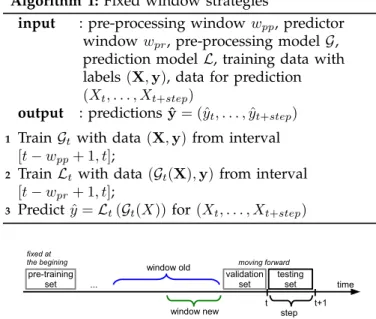
The fixed training window strategy can be applied to pre-processing as well. Suppose now we are at timet. We retrain our pre-processor with the historical data from the time interval[t−wpp+ 1, t], wherewpp is the length of the training window for the pre-processor. Then we retrain the predictor with the historical data from the time interval[t−wpr+ 1, t], wherewpr is the length of the training window for the predictor. Decoupling of the two adaptive components implies that the two training windows do not need to be equal. As demonstrated in this study, there may be situations where keepingwpp6= wpr may be beneficial to the prediction accuracy. The system for the predictions at timetis updated as defined in Algorithm 1.
Our prototype system uses four individual fixed win-dow strategies:
Algorithm 1:Fixed window strategies
input : pre-processing windowwpp, predictor windowwpr, pre-processing modelG, prediction modelL, training data with labels(X,y), data for prediction
(Xt, . . . , Xt+step)
output : predictionsyˆ= (ˆyt, . . . ,yˆt+step)
1 Train Gtwith data(X,y)from interval
[t−wpp+ 1, t];
2 Train Lt with data(Gt(X),y)from interval
[t−wpr+ 1, t];
3 Predictyˆ=Lt(Gt(X))for (Xt, . . . , Xt+step)
time pre-training set t window new window old testing set validation set step t+1 ... fixed at
the begining moving forward
Fig. 9. Setting of the selective windows strategy.
• ‘old-old’: wpp=wold and wpr=wold,
• ‘old-new’: wpp =wold and wpr=wnew,
• ‘new-new’:wpp=wnew andwpr=wnew, and
• ‘new-old’: wpp =wnew and wpr=wold,
where wold and wnew are two user input fixed training windows where wold> wnew.
4.2 Online strategy selection
In real online prediction tasks changes are likely to happen irregularly and unexpectedly, therefore, different length of training windows may be optimal at different times [13]. Our prototype system allows variable lengths of training windows by choosing at every time step one of the four strategies for the final prediction. The idea is to train the four strategies ‘old-old’, ‘old-new’, ‘new-new’, and ‘new-old’ simultaneously and evaluate them on a validation set before making the final predictions. We use the newest historical data for validation, assum-ing that this data closely reflects what we can expect in the nearest future. Figure 9 illustrates the setting. The procedure for selective window is defined in Algorithm 2. All four strategies are simultaneously trained, tested on the validation set, then the strategy that has the minimum validation error is selected and the models re-trained with this strategy to include the validation data, since we would not like to ‘throw away’ this newest labeled data after validation. The validation set changes continuously to reflect the latest data distribution. Next section presents experimental evaluation of this system. The idea of the model selection using cross validation is not new. Such strategies have been used in online learning with adaptive classifier ensembles [14], [15]. The novel part in this study is handling two adaptive components in the same prediction system.
Algorithm 2: Selective window strategy
input :wold,wnew,wval, pre-processing modelG, prediction model L, training data with labels
(X,y), data for prediction(Xt, . . . , Xt+step)
output: predictionsˆyt..t+step
1 TrainGold with (X,y)from
[t−wval−wold+ 1, t−wval]and Gnew with (X,y) from[t−wval−wnew+ 1, t−wval];
2 TrainLoldold with(Gold(X),y)from
[t−wval−wold+ 1, t−wval];
3 Loldnew with (Gold(X),y)from
[t−wval−wnew+ 1, t−wval];
4 Lnewold with (Gnew(X),y)from
[t−wval−wold+ 1, t−wval];
5 Loldold with (Gnew(X),y)from
[t−wval−wnew+ 1, t−wval];
6 TestLoldold,Lnewold(X),Loldnew(X),Lnewnew(X)on validation data from[t−wval+ 1, . . . , t];
7 PickLstrategy with min. validation error ;
8 RetrainGtwith (X,y)from[t−wppstrategy+ 1, t]and
Lt(X)with(Gt(X),y)from[t−wprstrategy+ 1, t];
9 Predictyˆ=Lt(Gt(X))for(Xt, Xt+step)
5
CASE STUDY WITH INDUSTRIAL DATA
We present a case study from chemical production do-main where we experimentally analyze the role of adap-tive pre-processing in online prediction systems. The purpose of our case study is to investigate the need and demonstrate the benefits of adaptive pre-processing. Our experiments have two goals. The first goal is to analyze and demonstrate the need for adaptive pre-processing to be decoupled from adaptive learning. The second goal is to assess a potential impact of adaptive pre-processing to the accuracy of an adaptive prediction system.
We do not claim that different training windows will always lead to more accurate results. Instead we argue and demonstrate with our numerical experiments and the case study that there may be algorithmic reasons why learning components in an adaptive system may need different phases of adaptation, even though they are a part of the same adaptive system, use data coming from the same source where changes happen at the same time.
5.1 Data
Existing benchmark data streams are not suitable for our study, as typically they are already pre-processed. For our experiments we need data that is as close to raw data as possible. Thus, we explore chemical production data (sensor readings), which are potentially noisy, changing and contain redundant variables, therefore they require acute pre-processing.
Our sensor reading data originates from a real chem-ical production process within Evonik Industries AG. The dataset covers nearly three years and consists of records of 85 real valued input variables measured every
10 20 30 40 50 60 70 80 90 block 1
block 2 block 3 block 4all
ID of the selected feature
Fig. 10. The need for adaptive feature selection.
5 minutes - 189 193 instances in total. The target variable is a real valued concentration of the production output. Minimizing concentration is the desired outcome of the production process. We formulate a classification task with this data, where the goal is to predict an increase or decrease in concentration as compared to the last observed period. The class balance is 50% : 50%.
Our data is not strictly raw data as it comes from a historical database which uses a lossy compression. The same compression algorithm is applied to all variables, thus the variables are not biased with respect to pre-processing we are applying in our experiments.
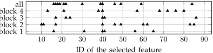
The following data exploration experiment motivates the need for adaptive pre-processing. We split our orig-inal data into four consecutive blocks (3 × 50 000 in-stances the first three blocks and the last 39 193 ) and run a supervised feature selection within each block sep-arately and then on the full dataset. Supervised feature selection first computes correlation between the target variable and each of the features, and then selects the features that have higher absolute correlation than a fixed threshold. Figure 10 indicates the selected features. If the same features were selected in all blocks, then we would see continuous vertical lines (like feature #40). We see that the optimal set of features changes from block to block of consecutive data, thus there is clearly a need for adaptive feature selection.
5.2 Experimental protocol
We perform three experiments that correspond to the situations A, B, C, described in Section 3, that motivate decoupling of adaptive pre-processing from adaptive predictor. For each experiment we test four fixed win-dow strategies ‘old-old’, ‘old-new’, old’ and ‘new-new’ (Algorithm 1), the selective strategy (Algorithm 2) and a non adaptive strategy ‘all’, which trains the pre-processor and the predictor at the beginning on a fixed chunk of data (2000 instances) and never updates later. The ‘all’ strategy serves as the baseline to verify if adaptive learning is needed at all. We expect this strategy to perform worse than the adaptive strategies.
Following the experiments in Section 3 we use the principal component analysis (situation A), feature nor-malization (situation B) and feature selection (situation C) as the pre-processor respectively. Since in our sce-narios we focus on training sample sizes for estimating the model parameters, we use a parametric classifier Naive Bayes as the main predictor. We complement
our experiments with Decision Tree as a non-parametric classifier and support vector machine (SVM) classifier as semi-parametric classifier.
In our data we do not know the change points or relevance of features in advance, the system needs to learn and fully adapt in an online mode. In Situation B we reduce the dimensionality of the problem from 86 to 21 by selecting every 4thfeature and run the experiment with four datasets that differ in sets of features (A: features#1,5,9, . . .are selected, B: features#2,6,10, . . ., C: features#3,7,11, . . ., D: features4,8,12, . . .).
In Situation C training is incremental. The old data is not accessible, thus we cannot retrain the predictor with the old data processed in the new way. As pre-processing we select 10 features that have the highest absolute correlation with the target variable in the last wnew instances. If some of the selected features remain the same as before, we keep them in the same positions in the pre-processed mapping of the data (i.e. if it was the second feature, it will stay the second feature). We update the models incrementally every 10 data points. At any point in time a new classifier may be started, but it cannot be trained with more than 10 latest historical data points. A new classifier can be used for prediction when it has been trained on wnew data points. We can pass the pre-processed data to this predictor using the old pre-processor (‘old-new’) or the new pre-processor (new’). For completeness we also test with ‘new-old’, where we feed the data pre-processed in the new way to the old predictor.
For evaluation we employ the test-then-train scenario, which processes data in the time order and simulates online arrival of data. First we test our strategies on a new incoming data chunk and record the testing results. Then we receive the true labels of this data chunk and use this data to update our learning components. We continue until the end of the data. We fix the size of chunk to 10 instances. If there is a tie in validation, the older model is used. We setwold= 600,wnew= 300.
The statistical significance of the differences in accu-racies was assessed using a non-parametric McNemar paired test, which does not require the assumption that the data is iid, therefore it is suitable for evolving data.
5.3 Analysis of accuracies
We first explore in depth the results with Naive Bayes as the base classifier and then complement the analysis with experiments using SVM and Decision Tree. 5.3.1 Results with Naive Bayes
Table 5 presents the results. The absolute accuracies are not very high, which is partially explainable by presence of compression in the dataset. Our primary interest in this case study is in analyzing the differences in accu-racies resulting from decoupled pre-processing rather than optimizing absolute accuracies. All the pairwise
differences are statistically significant except ‘all’ vs. ‘new-old’ in Situation B(1).
Overall, we observe that the non-adaptive ‘all’ achieves only around50%accuracy that is not better than the majority class classifier would achieve, that would assign all the instances to the same class. These results support the need for adaptive methods. The results ‘all’ are not equal across the situations as we use different pre-processing models for each situation.
TABLE 5
Accuracies (in%) with Naive Bayes.
Sit. all old-old old-new new-old new-new select
A 50.11 56.37 57.36 54.40 58.25 58.49 B(1) 49.56 49.56 56.69 50.67 56.69 58.15 B(2) 50.14 50.14 56.33 51.29 56.33 58.06 B(3) 50.19 50.19 56.73 51.58 56.73 58.89 B(4) 50.12 50.12 57.26 51.49 57.26 58.87 C 49.74 49.74 55.55 50.07 54.03 58.04
In Situation A the best performance is achieved by ‘select’, closely followed by ‘new-new’, which used short fixed windows. Further analysis, however, suggests that the best performing ‘select’ strategy did not rely on the shortest windows, quite the opposite, 58% of times it selected ‘old-old’ to make the final decision, 15% ‘old-new’, 17% ‘new-old’, and10%‘new-new’. These results confirm that selective handling of strategies is better than the fixed strategies. We also observe that the strategies which use decoupled training windows (‘old-new’ and ‘new-old’) are found to be optimal for more than30%of data points, therefore the idea of decoupling contributes substantially to the final superior accuracy.
Recall from Section 3 that in Situation B we do not update the old models. Therefore, in Situation B ‘old-old’ is the same as ‘all’. ‘old-new’ updates only the predictor, old’ updates only the pre-processor and ‘new-new’ updates both. In Situation B the ‘select’ strategy outperforms the fixed window strategies as well. Table 6 provides the counts of how many times a particular strategy was selected for the final decision making. The fixed strategy ‘new-old’ can be expected to perform well if the changes take place in such a way that the concepts move together. Such situation is not likely to hold over long period of time. We see that even though the fixed ‘new-old’ does not perform well when it is applied regularly, it is selected as the best performing strategy for13−18%of data points. The results confirm that situations in which this strategy appears to be the most accurate happen in the data, therefore the idea of decoupling is beneficial for improving the overall accuracy of the system.
In Situation C the ‘select’ strategy again performs the best and ‘old-new’ is the runner up. The performance of ‘old-new’ can be explained by the fact that the old pre-processing keeps the feature space stable and familiar for the old predictor. Even though retraining the processing alters the feature space and the old pre-processing may be sub-optimal for the new data, in
TABLE 6
Counts of selections in the ‘select’ strategy.
Sit. old-old old-new(=new-new) new-old
B(1) 55% 30% 15%
B(2) 57% 30% 13%
B(3) 53% 29% 18%
B(4) 55% 29% 16%
many cases the new pre-processing does not fit well with the existing predictor. The ‘select’ strategy overcomes this issue. The results confirm that even in our simple setting the system can make use of all combinations of old and new models. 59%of times ‘old-old’ model was selected,28% of times ‘old-new’ model, while ‘new-old’ and ‘new-new’ models were selected 3% and 10% of times respectively. The fact that for 13% of data points the model that uses the new pre-processing was selected suggests that decoupling may be beneficial even in this situation where it seems at first that such a strategy may harm the incremental predictor rather than help.
In summary, Table 7 presents the ranking of the strategies from the best performing to the worst. The ‘select’ strategy is leading in our prototype system. It demonstrates a great potential for further research of adaptive pre-processing in adaptive prediction systems. Our closer analysis of which strategies have been se-lected within the ‘select’ strategies confirms that the decoupled adaptivity in all three situation substantially contributes to improving the final accuracy.
TABLE 7
Ranking from the best to the worst.
Situation A Situation B Situation C
select select select
new-new new-new/old-new old-new
old-new new-old new-new
old-old all/old-new new-old
new-old all/old-new
all
5.3.2 Results with other base classifiers
In our experimental analysis the need for decoupled pre-processing was motivated by different learning rates of the pre-processors and the predictors. One could reasonably expect that the need for decoupling would manifest stronger when using parametric learning mod-els, since they need to accurately estimate their param-eters for optimizing the performance. In this section we experimentally analyze to what extent the learners that estimate the decision boundary directly can benefit from decoupling in our example cases. We investigate the performance of the prototype strategy with SVM (RBF kernel) and Decision Tree (Gini’s diversity index) as the predictors. The accuracies are presented in Table 8.
With SVM the following pairwise differences are not statistically significant: in Situation A old’ vs. ‘old-new’, Situation B(2) ‘all’ vs. ‘new-old’ and ‘new-old’
TABLE 8
Accuracies (in%) with SVM and Decision Tree.
SVM
Sit. all old-old old-new new-old new-new select
A 50.11 61.63 61.61 60.49 61.30 62.17 B(1) 50.11 50.11 53.81 50.09 53.81 55.93 B(2) 50.11 50.11 56.97 50.12 56.97 57.33 B(3) 50.11 50.11 57.79 50.13 57.79 57.79 B(4) 50.12 50.12 56.51 50.16 56.51 57.16 C 50.11 50.11 60.37 50.11 53.45 58.75 Decision Tree
Sit. all old-old old-new new-old new-new select
A 50.30 60.27 61.06 60.54 61.15 60.95 B(1) 50.97 50.97 63.96 50.08 63.96 60.96 B(2) 50.69 50.69 63.79 49.83 63.79 61.01 B(3) 50.09 50.09 64.07 49.76 64.07 61.03 B(4) 50.06 50.06 64.14 49.89 64.14 61.34 C 50.43 50.43 64.11 49.93 59.90 61.46
vs. old’, in Situation B(3) ‘all’ vs. ‘new-old’, ‘old-old’ vs. ‘old-old’, ‘old-new’ vs. ‘selective’ and ‘new-new’ vs. ‘selective’, in Situation C ‘all’ vs. ‘new-old’ and ‘old-old’ vs. ‘new-old’. With the Decision Tree only two differences are not statistically significant: in Situation B(4) ‘all’ vs. ‘new-old’ and ‘old-old’ vs. ‘new-old’.
In all situations the non-adaptive ‘all’ performs much worse than the adaptive strategies which confirms the need for adaptivity. To support the need for decoupling ‘select’, new’ or ‘new-old’ needs to outperform ‘old-old’ and ‘new-new’. We see that this happens in the results with SVM. Although in Situation C the ‘select’ strategy is not the best, even in this case the strategy that uses different adaptivity modes for the pre-processor and the predictor (‘old-new’) wins. In the Decision Tree experiments, however, we see the ‘new-new’ strategy performing equally well. That can be attributed to the non-parametric nature of the Decision Tree classifier, in that case the training sample size does not matter that much for accurate estimation of the parameters, as mat-ters the learning from the newest data. In Situation C we observe that the decoupled adaptivity (‘old-new’) gives the most accurate results. Overall, the results justify that even for non-parametric learning model there are situations in which decoupled adaptive pre-processing is beneficial towards the final accuracy.
6
R
ELATED WORKTo the best of our knowledge this work is the first to address the issue of adaptive pre-processing when learning from evolving streaming data. It is also the first to raise the issue of synchronizing multiple adaptive components in one online learning system when the components adapt at different phases.
Several studies address the problem of adaptive fea-ture space (but not pre-processing in general). A few works on adaptive feature selection tackle specific prob-lems. Several works originating from different research groups relate to classifying textual streams [16]–[18]. Learning from textual data online requires adaptive
feature space, since in the TF-IDF representation of textual data the attributes relate to words, while the number of words (and so the attributes) is potentially unlimited. New attributes may appear and of course the relevance of attributes changes over time. These works study how to incorporate new features incrementally, which is straightforward for classifiers that deal with individual attributes separately, such as Naive Bayes. These approaches can be considered as a special case in our reference framework, namely Scenario S3 under
incremental learning mode.
Another series of works [19], [20] consider dynamic feature selection in data streams. They specifically work with regression problems. These works relate via chang-ing environment and dynamic feature selection key-word; however, the setting is different there. These works can be considered as active learning in attribute space, where the approaches actively select which at-tributes to observe next. Thus, the resulting historical data has a lot of values missing on purpose and these works focus on how to handle that.
Adaptive pre-processing has been addressed in sta-tionary online learning [21] for another specific problem, namely, normalization of the input variables in online learning for neural networks so that they fall into range
[−1,1]. The proposed approach links scaling of features with scaling of weights. In this case, however, the pre-processor is not adaptive. This study rather investigates the environment in which the neural network itself as a predictor can or cannot be adaptive.
7
C
ONCLUSIONWe raised the issue of adaptive pre-processing in evolv-ing data. We challenged one of the major assumptions in adaptive learning research, which assumes that data comes already pre-processed or that pre-processing is an integral part of a learning algorithm implying that there is no need for adaptive pre-processing.
We identified three scenarios where decoupling adap-tive pre-processing and adapadap-tive learning may be ben-eficial. We demonstrated that the situations in which decoupling the adaptivity of pre-processing and the predictor may benefit the final accuracy.
We presented a prototype approach that handles adap-tivity of pre-processing and adapadap-tivity of predictor sepa-rately. Our case study with real production data demon-strated that the proposed prototype approach may help to improve the prediction accuracy.
We identified practically important directions for fur-ther research to be addressed in the forthcoming re-search. Firstly, it is urgent to investigate how to properly integrate the adaptivity of two components in a single system to exploit the benefits of the decoupled adaptivity of the two. Secondly, it is important to investigate how to monitor and detect the need for adapting pre-processor in very high dimensional spaces under constraints im-plied by the computational resources.
A
CKNOWLEDGMENTThe authors than Evonik Industries for providing the data. The research leading to these results has received funding from the European Commission within the Marie Curie Industry and Academia Partnerships & Pathways (IAPP) programme under grant agreement no. 251617.
R
EFERENCES[1] A. Bifet, G. Holmes, B. Pfahringer, R. Kirkby, and R. Gavalda, “New ensemble methods for evolving data streams,” inProc. of the 15th ACM SIGKDD int. conf. on Knowledge discovery and data mining (KDD’09), 2009, pp. 139–148.
[2] E. Ikonomovska, J. Gama, and S. Dzeroski, “Learning model trees from evolving data streams,” Data Mining Knowledge Discovery, pp. 1–41, 2010.
[3] P. Kadlec and B. Gabrys, “Architecture for development of adap-tive on-line prediction models,”Memetic Computing, vol. 1, no. 4, pp. 241–269, 2009.
[4] M. Masud, J. Gao, L. Khan, J. Han, and B. Thuraisingham, “Classification and novel class detection in concept-drifting data streams under time constraints,”IEEE Trans. on Knowl. and Data Eng., vol. 23, pp. 859–874, 2011.
[5] J. Kolter and M. Maloof, “Dynamic weighted majority: An en-semble method for drifting concepts,”J. Mach. Learn. Res., vol. 8, pp. 2755–2790, December 2007.
[6] L. Minku, A. White, and X. Yao, “The impact of diversity on online ensemble learning in the presence of concept drift,”IEEE Trans. on Knowl. and Data Eng., vol. 22, pp. 730–742, 2010.
[7] T. Breur. (2007) Toms ten data tips. [Online].
Available: http://www.xlntconsulting.com/newsletter-archive/ data-preparation-december-2007.html
[8] I. Witten, E. Frank, and M. Hall,Data Mining: Practical Machine Learning Tools and Techniques (3rd Ed.). Morgan Kaufmann, 2011. [9] E. Bingham and H. Mannila, “Random projection in dimension-ality reduction: applications to image and text data,” in Proc. of the seventh ACM SIGKDD international conference on Knowledge discovery and data mining. ACM, 2001, pp. 245–250.
[10] G. Widmer and M. Kubat, “Effective learning in dynamic environ-ments by explicit context tracking,” inProceedings of the European Conference on Machine Learning (ECML’93)s. Springer-Verlag, 1993, pp. 227–243.
[11] M. Masud, Q. Chen, L. Khan, C. Aggarwal, J. Gao, J. Han, and B. Thuraisingham, “Addressing evolution in concept-drifting data streams,” inProc. of the 10th IEEE Int. Conf. on Data Mining (ICDM’10), 2010.
[12] G. Widmer and M. Kubat, “Learning in the presence of concept drift and hidden contexts,”Mach. Learn., vol. 23, pp. 69–101, 1996. [13] I. ˇZliobait ˙e, “Adaptive training set formation,” Ph.D. dissertation,
Vilnius University, 2010.
[14] R. Klinkenberg, “Learning drifting concepts: Example selection vs. example weighting,”Intell. Data Anal., vol. 8, pp. 281–300, 2004. [15] A. Tsymbal, M. Pechenizkiy, P. Cunningham, and S. Puuronen,
“Dynamic integration of classifiers for handling concept drift,” Inf. Fusion, vol. 9, pp. 56–68, 2008.
[16] M. M. Q. Chen, J. Gao, L. Khan, J. Han, and B. Thuraisingham, “Classification and novel class detection of data streams in a dy-namic feature space,” inProceedings of the 2010 European conference on Machine learning and knowledge discovery in databases: Part II, ser. ECML PKDD’10. Springer-Verlag, 2010, pp. 337–352.
[17] I. Katakis, G. Tsoumakas, and I. Vlahavas, “Dynamic feature space and incremental feature selection for the classification of textual data streams,” in Proceedings of ECML/PKDD-2006 International Workshop on Knowledge Discovery from Data Streams. Springer Verlag, 2006, pp. 107–116.
[18] B. Wenerstrom and C. Giraud-Carrier, “Temporal data mining in dynamic feature spaces,” inProceedings of the Sixth International Conference on Data Mining, ser. ICDM ’06. IEEE Computer Society, 2006, pp. 1141–1145.
[19] C. Anagnostopoulos, D. Tasoulis, D. Hand, and N. Adams, “Online optimization for variable selection in data streams,” in Proceeding of the 2008 conference on ECAI 2008: 18th European Conference on Artificial Intelligence. IOS Press, 2008, pp. 132–136.
[20] C. Anagnostopoulos, N. Adams, and D. Hand, “Deciding what to observe next: adaptive variable selection for regression in mul-tivariate data streams,” inProceedings of the 2008 ACM symposium on Applied computing, ser. SAC ’08. ACM, 2008, pp. 961–965. [21] H. Ruda, “Adaptive preprocessing for on-line learning with
adap-tive resonance theory (art) networks,” in Proc. of the 1995 IEEE Workshop on Neural Networks for Signal Processing (NNSP.
Indr ˙e Zliobait ˙eˇ is a Lecturer in Computational Intelligence at Bournemouth University UK. She received her PhD from Vilnius Uni-versity, Lithuania in 2010. I. ˇZliobait ˙e has six years of experience in credit analysis in banking industry. Her research interests concentrate around online data mining, including learning from evolving streaming data, change detection, adaptive and context-aware learning, predic-tive analytics applications. Recently she has co-chaired workshops at ECMLPKDD 2010 and ICDM 2011, co-organized tutorials at CBMS 2010 and PAKDD 2011 on adaptive learning. She is a Research Task Leader within the INFER.eu project that is developing evolving and robust predictive systems. For further information see
http://zliobaite.googlepages.com.
Bogdan Gabrysreceived an MSc in electronics and telecommunication from Silesian Technical University, Poland, in 1994, and a PhD in com-puter science from Nottingham Trent University, UK, in 1998. After many years of working at different Universities, he moved to the Bournemouth University in January 2003, where he holds a Chair in Computational Intelligence position and acts as a director of the Smart Technology Re-search Centre within the School of Design, Engineering and Computing. Prof. Gabrys was the proposer and is the coordinator of the INFER.eu project within which the work reported in this manuscript originated. His current research interests lay in a broad area of intelligent, com-plex adaptive systems and include a wide range of machine learning, biologically/nature inspired learning and hybrid intelligent techniques encompassing data and information fusion, learning and adaptation methods, multiple classifier and prediction systems, processing and modelling of uncertainty in predictive modelling, pattern recognition, diagnostic analysis and decision support systems.