Bayesian Multi-Task Reinforcement Learning
Alessandro Lazaric, Mohammad Ghavamzadeh
To cite this version:
Alessandro Lazaric, Mohammad Ghavamzadeh. Bayesian Multi-Task Reinforcement Learning.
ICML - 27th International Conference on Machine Learning, Jun 2010, Haifa, Israel.
Omni-press, pp.599-606, 2010.
<inria-00475214>
HAL Id: inria-00475214
https://hal.inria.fr/inria-00475214
Submitted on 21 Apr 2010
HAL
is a multi-disciplinary open access
archive for the deposit and dissemination of
sci-entific research documents, whether they are
pub-lished or not.
The documents may come from
teaching and research institutions in France or
abroad, or from public or private research centers.
L’archive ouverte pluridisciplinaire
HAL
, est
destin´
ee au d´
epˆ
ot et `
a la diffusion de documents
scientifiques de niveau recherche, publi´
es ou non,
´
emanant des ´
etablissements d’enseignement et de
recherche fran¸cais ou ´
etrangers, des laboratoires
publics ou priv´
es.
Bayesian Multi-Task Reinforcement Learning
Alessandro Lazaric Mohammad Ghavamzadeh
INRIA Lille - Nord Europe, Team SequeL, France
{alessandro.lazaric,mohammad.ghavamzadeh}@inria.fr
Abstract
We consider the problem of multi-task reinforcement learning where the learner is provided with a set of tasks, for which only a small number of samples can be generated for any given policy. As the number of samples may not be enough to learn an accurate evaluation of the policy, it would be necessary to identify classes of tasks with similar structure and to learn them jointly. We consider the case where the tasks share structure in their value functions, and model this by assum-ing that the value functions are all sampled from a common prior. We adopt the Gaussian process temporal-difference value function model and use a hierarchical Bayesian approach to model the distribution over the value functions. We study two cases, where all the value functions belong to the same class and where they belong to an undefined number of classes. For each case, we present a hierarchi-cal Bayesian model, and derive inference algorithms for (i) joint learning of the value functions, and (ii) efficient transfer of the information gained in (i) to assist learning the value function of a newly observed task.
1
Introduction
Multi-task learning (MTL) is an important learning paradigm and has recently been an area of active research in machine learning (e.g., [4; 1; 17; 16; 3]). A common setup is that there are multiple related tasks for which we are interested in improving the performance over individual learning by sharing information across the tasks. This transfer of information is particularly important when we are provided with only a limited number of data to learn each task. Exploiting data from related problems provides more training samples for the learner and can improve the performance of the resulting solution.
Most reinforcement learning (RL) algorithms [2; 13] often need a large number of samples to solve a problem and cannot directly take advantage of the information coming from other similar tasks. Nonetheless, recent work has shown that transfer and multi-task learning techniques can be em-ployed in RL to reduce the number of samples needed to achieve nearly-optimal solutions. All approaches to multi-task RL (MTRL) assume that the tasks share similarity in some components of the problem such as dynamics, reward structure, or value function. While some methods explic-itly assume that the shared components are drawn from a common generative model [15; 10], this assumption is more implicit in others [14; 9]. In [10], tasks share the same dynamics and reward features, and only differ in the weights of the reward function. The proposed method initializes the value function for a new task using the previously learned value functions as a prior. In [15], the distribution over the dynamics and the reward functions of the tasks is drawn from a hierarchical Bayesian model (HBM). Due to some similarity to our work, we discuss this method in more de-tails in Section 5. In [9], the authors implicitly assume that the tasks are drawn from a common distribution. They propose a method to selectively transfer samples from source tasks to a target task based on the likelihood of the target samples being generated by the models built for the source tasks. Finally, in [14], learning the value function of the target task is expedited using the solution learned in a source task with related, but different, state and action spaces.
In this paper, we study the MTRL scenario in which the learner is provided with a number of tasks with common state and action spaces. For any given policy, only a small number of samples can be generated in each task, which may not be enough to accurately evaluate the policy. In such a MTRL problem, it is necessary to identify classes of tasks with similar structure and to learn them jointly. In our work, we consider a particular class of MTRL problems in which the tasks share structure in their value functions. To allow the value functions to share a common structure, one way would be to assume that they are all sampled from a common prior. We adopt the Gaussian process temporal-difference (GPTD) value function model [6] for each task, model the distribution over the value functions using a HBM, and develop solutions to the following problems: (i) joint learning of the value functions, and (ii) efficient transfer of the information acquired in (i) to facilitate learning the value function of a newly observed task. We refer to the above problems as symmetric and asymmetric multi-task learning, respectively. In Section 3, we present a HBM for the case in which all the value functions belong to the same class, and derive an EM algorithm to find MAP estimates of the value functions and the model’s hyper-parameters. However, as pointed out in [4; 1], if the functions do not belong to the same class, simply learning them together can be detrimental (negative transfer). It is therefore important to have models that will generally benefit from related tasks and will not hurt performance when the tasks are unrelated. This is particularly important in RL as changing the policy at each step of the policy iteration algorithm (this is true even for the fitted value iteration algorithm) can change the way tasks are clustered together. This means that even if we start with value functions that all belong to the same class, after one iteration the new value functions may be clustered into several classes. In Section 4, we introduce a Dirichlet process (DP) based HBM for the case that the value functions belong to an undefined number of classes, and derive inference algorithms for both the symmetric and asymmetric scenarios. In Section 5, we discuss the similarities and differences with closely related work. In Section 6, we report and analyze experimental results.
2
Preliminaries
The agent-environment interaction in RL is conventionally modelled as a Markov Decision Process (MDP). A MDP is a tupleM = hX,A,R,Pi whereX andAare the state and action spaces, respectively;Ris the probability distribution over rewardsR; andP is the transition probability distribution. A stationary policyπ : X × A →[0,1]is a mapping from states to action selection probabilities. The MDP controlled by a policyπinduces a Markov chain with transition probability distributionPπ(x′
|x) = RAP(x
′
|x, a)π(a|x)da. Given a policyπ, the (possibly discounted,γ ∈
[0,1)) return for a statex,Dπ(x), is a random process defined byDπ(x) =P∞
t=0γtR(xt)|x0 =
x, with xt+1 ∼ Pπ(·|xt). The value functionVπ(x)is the expected value of Dπ(x)where the
expectation is over all possible trajectories and rewards collected along them.
A key problem in RL is to learn the value function of a given policy, which is called policy
evalu-ation [2; 13]. Loosely speaking, in policy evaluevalu-ation the goal is to find a “close enough”
approx-imationV of the value functionVπ. Unlike in supervised learning, the target functionVπ is not
known in advance and its values have to be inferred from the observed rewards. Therefore, it is required to define a stochastic generative model connecting the underlying hidden value function with the observed rewards. In this paper, we adopt the GPTD value function model proposed in [6], in which the discounted returnDis decomposed into its meanV and a random zero-mean residual ∆V,D(x) =V(x) + ∆V(x). Combining this decomposition with the Bellman equation, we obtain
R(x) =V(x)−γV(x′ ) +ǫ(x, x′ ), x′ ∼Pπ(·|x), (1) where ǫ(x, x′ ) def= ∆V(x)−γ∆V(x′
). Suppose we are provided with a set of samples D =
{(xn, x′n, rn)}Nn=1, wherernandx′n are the reward and the next state observed by following
pol-icyπ in statexn, respectively. By writing the model of Eq. (1) w.r.t. these samples, we obtain
R=HV +E, where H∈RN×2N and R⊤= (rn)Nn=1; E ⊤ = ǫ(xn, x′n) N n=1; V ⊤ = V(xn), V(x′n) N n=1
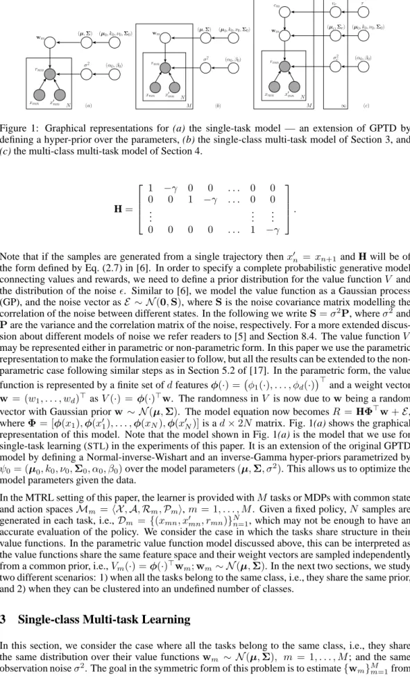
(a) xmn N wm rmn σ 2 (µ,Σ) (α0, β0) (µ0, k0, ν0,Σ0) x′ mn (b) xmn N wm rmn M σ2 (α0, β0) (µ0, k0, ν0,Σ0) (µ,Σ) x′ mn (c) xmn N cm wm rmn M ∞ vc σ2 c (µc,Σc) (α0, β0) τ (µ0, k0, ν0,Σ0) x′ mn
Figure 1: Graphical representations for (a) the single-task model — an extension of GPTD by defining a hyper-prior over the parameters, (b) the single-class multi-task model of Section 3, and
(c) the multi-class multi-task model of Section 4.
H= 1 −γ 0 0 . . . 0 0 0 0 1 −γ . . . 0 0 .. . ... ... 0 0 0 0 . . . 1 −γ .
Note that if the samples are generated from a single trajectory thenx′
n =xn+1 and H will be of
the form defined by Eq. (2.7) in [6]. In order to specify a complete probabilistic generative model connecting values and rewards, we need to define a prior distribution for the value functionV and the distribution of the noiseǫ. Similar to [6], we model the value function as a Gaussian process (GP), and the noise vector asE ∼ N(0,S), whereSis the noise covariance matrix modelling the correlation of the noise between different states. In the following we writeS=σ2P, whereσ2and Pare the variance and the correlation matrix of the noise, respectively. For a more extended discus-sion about different models of noise we refer readers to [5] and Section 8.4. The value functionV may be represented either in parametric or non-parametric form. In this paper we use the parametric representation to make the formulation easier to follow, but all the results can be extended to the non-parametric case following similar steps as in Section 5.2 of [17]. In the non-parametric form, the value function is represented by a finite set ofdfeaturesφ(·) = φ1(·), . . . , φd(·)
⊤
and a weight vector
w = (w1, . . . , wd)⊤asV(·) = φ(·)⊤w
. The randomness in V is now due towbeing a random vector with Gaussian priorw ∼ N(µ,Σ). The model equation now becomesR =HΦ⊤w+E, whereΦ= [φ(x1),φ(x′1), . . . ,φ(xN),φ(x′N)]is ad×2N matrix. Fig. 1(a) shows the graphical representation of this model. Note that the model shown in Fig. 1(a) is the model that we use for single-task learning (STL) in the experiments of this paper. It is an extension of the original GPTD model by defining a Normal-inverse-Wishart and an inverse-Gamma hyper-priors parametrized by ψ0= (µ0, k0, ν0,Σ0, α0, β0)over the model parameters(µ,Σ, σ2). This allows us to optimize the
model parameters given the data.
In the MTRL setting of this paper, the learner is provided withM tasks or MDPs with common state and action spacesMm =hX,A,Rm,Pmi,m= 1, . . . , M. Given a fixed policy,N samples are
generated in each task, i.e.,Dm = {(xmn, x′mn, rmn)}Nn=1, which may not be enough to have an
accurate evaluation of the policy. We consider the case in which the tasks share structure in their value functions. In the parametric value function model discussed above, this can be interpreted as the value functions share the same feature space and their weight vectors are sampled independently from a common prior, i.e.,Vm(·) =φ(·)⊤wm;wm∼ N(µ,Σ). In the next two sections, we study
two different scenarios: 1) when all the tasks belong to the same class, i.e., they share the same prior, and 2) when they can be clustered into an undefined number of classes.
3
Single-class Multi-task Learning
In this section, we consider the case where all the tasks belong to the same class, i.e., they share the same distribution over their value functionswm ∼ N(µ,Σ), m = 1, . . . , M; and the same observation noiseσ2. The goal in the symmetric form of this problem is to estimate{w
the data{Dm}Mm=1, whereas in the asymmetric case we are interested in estimating the parameters
θ = (µ,Σ, σ2) from the data in order to use them as a prior for a newly observed task (e.g., task MM+1). We use a parametric HBM for this problem. HBMs allow us to model both the
individuality of the tasks and the correlation between them. In HBMs, individual models with task specific parameters are usually located at the bottom, and at the layer above, tasks are connected together via a common prior placed over those parameters. Learning the common prior is a part of the training process in which data from all the tasks contribute to learning, thus making it possible to share information between the tasks usually via sufficient statistics. Then given the learned prior, individual models are learned independently. As a result, learning at each task is affected by both its own data and by data from the other tasks related through the common prior.
3.1 The Model
We assume a normal-inverse-Wishart and an inverse-Gamma hyper-priors for(µ,Σ)andσ2,
re-spectively.
p(θ|ψ0) =p(µ,Σ) × p(σ2) =N(µ;µ0,Σ/k0)IW(Σ;ν0,Σ0) × IG(σ2;α0, β0). (2)
These distributions are the conjugate priors for multivariate Gaussian distributionsp(wm|µ,Σ)and p(Rm|wm, σ2) = N(HΦ
⊤
mwm, σ2P), respectively. This leads to the following generative model
for the data,{Dm}. Fig. 1(b) shows the graphical representation of this model. The details of the
model can be found in Section 8.
Single-Class Model: Given the hyper-parametersψ0= (µ0, k0, ν0,Σ0, α0, β0),
1. The parametersθ= (µ,Σ, σ2)are sampled once from the hyper-prior as in Eq. (2),
2. For each taskMm(value functionVm), the weight vector is sampled aswm∼ N(µ,Σ),
3. Given{(xmn, x′mn)}Nn=1, we haveRm =HΦ⊤mwm+E, whereE ∼ N(0, σ2P), m=
1, . . . , M.
3.2 Inference
This model can be learned by optimizing the penalized likelihoodp {Rm}|{(xmn, x′mn)}, θ
p(θ) w.r.t. the parametersθ = (µ,Σ, σ2)using an EM algorithm. In the rest of the paper, we refer to this algorithm asSCMTL, for single-class multi-task learning.
E-step: Since the posterior distribution of the latent variables p({wm}|{Dm}, θ) is a prod-uct ofM Gaussian posterior distributionsp(wm|Dm, θ) = N(µ′
0m,Σ
′
0m), for each taskm, we
compute the mean and covariance as
µ′0m=Σ ′ 0m 1 σ2ΦmH ⊤ P−1Rm+Σ−1µ , Σ′0 m= 1 σ2ΦmH ⊤ P−1HΦ⊤m+Σ−1 −1 .
M-step: We optimize θ to maximize the penalized expected log-likelihood of complete data logp {Dm},{wm}|θover the posterior distribution estimated in the E-step and obtain the new
parameters µnew= 1 M+k0 k0µ0+ M X m=1 µ′0m ! , Σnew= 1 M+ν0+d+ 2 ( k0(µ−µ0)(µ−µ0) ⊤+Σ0+ M X m=1 h (µ′ 0m−µ)(µ ′ 0m−µ) ⊤ +Σ′0m i) , σ2new= 1 M N+ 2(1 +α0) ( 2β0+ M X m=1 trP−1HΦm⊤Σ′0mΦmH⊤ +Rm−HΦ⊤mµ′0m P−1Rm−HΦ⊤mµ′0m ⊤) .
4
Multi-class Multi-task Learning
In this section, we consider the case where the tasks belong to an undefined number of classes. Tasks in the same class{Mm| cm = c} share the same distribution over their value functions
wm ∼ N(µ
c,Σc), and the same observation noiseσ2c. We use a nonparametric HBM for this
problem. In the HBM proposed in this paper, the common prior is drawn from a Dirichlet process (DP). As addressed in the statistics literature (see, e.g., [11]), DP is powerful enough to model the parameters of individual classes, to fit them well without any assumption about the functional form of the prior, and to automatically learn the number of underlying classes.
4.1 The Model
We place a DP(τ, G0)prior over the class assignment and the class parameters. The concentration
parameterτ and the base distributionG0 can be considered as priors over the number of classes
and the class parameters θc = (µc,Σc, σ2c), respectively. G0 is specified as the product of a
d-dimensional normal-inverse-Wishart and a 1-dimensional inverse-Gamma distributions, with parametersψ0= (µ0, k0, ν0,Σ0, α0, β0), (see Eq. 2). We employ the stick-breaking representation
of the DP prior [7], and define a task-to-class assignment variable(cm1, . . . , cm∞)for each taskm,
whose elements are all zero except that thecth element is equal to one if taskmbelongs to classc. Given the above, the data{Dm}can be seen as drawn from the following generative model, whose
graphical representation is shown in Fig. 1(c).
Multi-Class Model: Given the hyper-parameters(τ, ψ0),
1. Stick-breaking view: Draw vc from the Beta distribution Be(1, τ), compute πc =
vcQc −1
i=1(1−vi), and independently drawθc∼G0, c= 1, . . . ,∞,
2. Task-to-class assignment: Draw the indicator(cm1, . . . , cm∞)from a multinomial
distri-butionM∞(1;π1, . . . , π∞), m= 1, . . . , M,
3. The weight vector is sampled aswm∼ N(µc
m,Σcm), m= 1, . . . , M,
4. Given{(xmn, x′mn)}Nn=1, we haveRm=HΦ⊤mwm+E, whereE ∼ N(0, σc2mP), m= 1, . . . , M.
4.2 Inference
We are interested in the posterior distribution of the latent variables Z = {wm},{cm},{θc}
given the observed data and the hyper-parameters τ and ψ0, i.e., p Z|{Dm}, τ, ψ0 ∝
p {Dm}|Z, τ, ψ0p(Z|τ, ψ0). In the following we outline the main steps of the algorithm used to
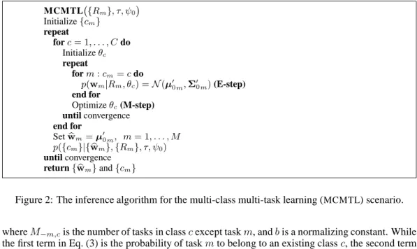
solve this inference problem, which we refer to asMCMTL, for multi-class multi-task learning (see Fig. 2). MCMTLcombines theSCMTLalgorithm of Sec. 3.2 for class parameters estimation, with a Gibbs sampling algorithm for learning the class assignments [12]. The main advantage of such combination is that at each iteration, given the current estimate of the weights, we take advantage of the conjugate priors to derive an efficient Gibbs sampling procedure.
More formally, given an arbitrary initial class assignment {cm}, a distinct EM algorithm is run
on each classc = 1, . . . , C (withC the current estimate of the number of classes) and returns M distributionsN(µ′
0m,Σ
′
0m). Given the weights estimated at the previous step,wbm = µ′0m,
the Gibbs sampling solves the DP inference by drawing samples from the posterior distribution p {cm}|{Rm},{wbm}, τ, ψ0
. In particular, the state of the Markov chain simulated in the Gibbs sampling is the class assignment{cm}, i.e., the vector of the classes each task belongs to. At each
iteration, each componentcmof the state is updated by sampling from the following distribution
Ifc=cm′, m′6=m: p cm=c|{cm′}, Rm,wbm, τ, ψ0=b M−m,c M−1 +τ Z p Rm,wbm|θcp θc|{cm′}, ψ0dθc, else:p cm6=cm′, m′6=m|{cm′}, Rm,wbm, τ, ψ0=b τ M−1 +τ Z p(Rm,wbm|θ)p(θ|ψ0)dθ, (3)
MCMTL {Rm}, τ, ψ0 Initialize{cm} repeat forc= 1, . . . , Cdo Initializeθc repeat form:cm=cdo p(wm|Rm, θc) =N(µ′ 0m,Σ′0m)(E-step) end for Optimizeθc(M-step) until convergence end for Setwbm=µ′ 0m, m= 1, . . . , M p({cm}|{wbm},{Rm}, τ, ψ0) until convergence return{wbm}and{cm}
Figure 2: The inference algorithm for the multi-class multi-task learning (MCMTL) scenario.
whereM−m,cis the number of tasks in classcexcept taskm, andbis a normalizing constant. While
the first term in Eq. (3) is the probability of taskmto belong to an existing classc, the second term returns the probability of assigning taskmto a new class. Thanks to the conjugate base distribution G0, the integrals in Eq. (3) can be solved analytically. In fact
p(Rm,wbm|θ)p(θ|ψ0) =p(Rm|wbm, σ2)p(wbm|µ,Σ)×p(µ,Σ|µ0, k0, ν0,Σ0)p(σ2|α0, β0) ∝ N(µ;µ′0,Σ/k ′ 0)IW(Σ;ν ′ 0,Σ ′ 0)× IG(σ2;α ′ 0, β ′ 0), (4) whereψ′ 0 = (µ ′ 0, k ′ 0, ν ′ 0,Σ ′ 0, α ′ 0, β ′
0)are the posterior parameters ofG0given the weightwbmand
the rewardsRm(see Section 8 for their definition). Using the posterior hyper-parameters, the second
integral in Eq. (3) can be written as
Z p(Rm,wbm|θ)p(θ|ψ0)dθ= k0 πk′ 0 d 2 |Σ 0|ν0/2 |Σ′ 0|ν ′ 0/2 Γν0′ 2 Γν0′−d 2 ×(2π|P|)−N2 β α0 0 Γ(α0) Γ(α′ 0) β′α′0 0 . (5)
In the first integral of Eq. (3), the density functionp(θc|{cm′}, ψ0)is the posterior probability over
the class parametersθc given the data from all the tasks belonging tocmaccording to the current
class assignment{cm′}. Similar to Eq. (4), we compute the posterior hyper-parametersψ0c of the
normal-inverse-Wishart and inverse-Gamma distributions given{wbm′}and{Rm′}, withm′6= m
andcm′ =cm. Finally, the integral can be analytically calculated as in Eq. (5), where the
hyper-parametersψ0and the posterior hyper-parametersψ0′ are replaced byψ0candψ0′c, respectively. 4.3 Symmetric vs. Asymmetric Learning
TheMCMTLalgorithm returns both the distribution over the weights for each task and the learned hierarchical model (task-class assignments). While the former can be used to evaluate the learn-ing performance in the symmetric case, the latter provides a prior for learnlearn-ing a new task in the asymmetric scenario.
Symmetric Learning. According to the generative model in Section 4.1, the task weights are
dis-tributed according to the normal distribution N(µ′0m,Σ ′
0m), whereµ ′
0m and Σ
′
0m are the
pos-terior mean and covariance of the weight vector wm returned by theMCMTL algorithm. Since Vm(x) =φ(x)
⊤
wm, the value ofVmat a test statex∗is distributed as
p Vm(x∗)|x∗,µ′0m,Σ′0m=N φ(x∗) ⊤ µ′0m, φ(x∗) ⊤ Σ′ 0 −1 mφ(x∗).
IfMCMTLsuccessfully clusters the task, we expect the value function prediction to be more accurate than learning each task independently.
Asymmetric Learning. In the asymmetric setting the class of the new task is not known in advance.
The inference problem is formalized asp wM+1|RM+1, ψ0,{cm}Mm=1
, wherewM+1andRM+1
are the weight vector and rewards of the new taskMM+1, respectively. Similar to Section 4.2, this
inference problem cannot be solved in closed form, thus, we must apply theMCMTLalgorithm to the new task. The main difference with the symmetric learning is that the class assignments{cm}
and weights{wbm}for all the previous tasks are kept fixed, and are used as a prior over the new task
learned by theMCMTLalgorithm. As a result, the Gibbs sampling reduces to a one-step sampling process assigning the new task either to one of the existing classes or to a new class. IfMM+1
belongs to a new class, then the inference problem becomesp(wM+1|RM+1, ψ0), that is exactly
the same as inSTL. On the other hand, ifMM+1belongs to classc, the rewards and weights{Rm′},
{wm′}of the tasks in classccan be used to compute the posterior hyper-parametersψ′0cas in Eq.
(4), and to solve the inference problemp(wM+1|RM+1, ψ′0c).
5
Related Work
In RL, the approach of this paper is mainly related to [15]. Although we both use a DP-based HBM to model the distribution over the common structure of the tasks, in [15] the tasks share structure in their dynamics and reward function, while we consider the case that the similarity is in the value function. There are scenarios in which significantly different MDPs and policies may lead to very similar value functions. In such scenarios, the method proposed in this paper would still be able to leverage on the commonality of the value functions, thus performing better than single-task learning. Moreover in [15], the setting is incremental, i.e., the tasks are observed as a sequence, and there is no restriction on the number of samples generated by each task. The focus is not on joint learning with finite number of samples, it is on using the information gained from the previous tasks to facilitate learning in a new one. This setting is similar to the asymmetric learning considered in our work. In supervised learning, our work is related to [17] and [16]. In [17], the authors present a single-class HBM for learning multiple related functions using GPs. Our single-class model of Section 3 is an adaptation of this work for RL using GPTD. Besides, our multi-class model of Section 4 extends this method to the case with an undefined number of classes. In [16], a DP-based HBM is used to learn the extent of similarity between classification problems. The problem considered in our paper is regression, the multi-class model of Section 4 is more complex than the one used in [16], and the inference algorithms of Section 4 are based on Gibbs sampling, where a variational method is used for inference in [16].
6
Experiments
In this section, we report empirical results applying the Bayesian multi-task learning (BMTL) al-gorithms presented in this paper to a regression problem and a benchmark RL problem, inverted pendulum. We compare the performance of single-task learning (STL) with single-class multi-task learning (SCMTL), i.e., all tasks are assumed to belong to the same class, and multi-class multi-task learning (MCMTL), i.e., tasks belong to a number of classes not known in advance. By STL, we refer to running the EM algorithm of Section 3.2 for each task separately. The reason to use the regression problem in our experiments is that it allows us to evaluate ourBMTLalgorithms when the tasks are generated exactly according to the generative models of Sections 3 and 4.
6.1 A Regression Problem
In this problem, tasks are functions in the linear space spanned by a feature space φ(x) = 1, x, x2
, x3
, x4
, x5
)⊤ on the domainX = [−1,1]. The weights for the tasks are drawn from four
different classes, i.e., four6-dim multivariate Gaussian distributions, with the parameters shown in Fig. 3(a). The noise covariance matrixS=diag(σ2
)for all the algorithms. We evaluate the perfor-mance of eachBMTLalgorithm by computing its relative mean squared error (MSE) improvement overSTL:(M SESTL−M SEBMTL)/M SESTL. The MSEs are computed overN′= 1000test samples.
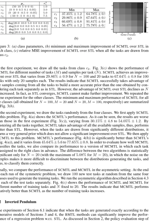
µc σ2c c1 (50 10 5 0 0 0) 1.0 c2 (0 0 0 0.5 0.1 0.05) 3.0 c3 (0-20 0 -0.5 0-0.05) 5.0 c4 (-50 0-5 0-0.1 0) 7.5 Σc c1 diag(20.0 10.0 5.0 0.0 0.0 0.0) c2 diag(0.0 0.0 0.0 0.5 0.1 0.05) c3 diag(0.0 5.0 0.0 0.5 0.0 0.01) c4 diag(20.0 0.0 5.0 0.0 0.1 0.0) Min Max c1 37.35%±1.2 64.78%±0.9 c2 29.86%±0.9 67.64%±0.8 c3 66.69%±0.8 91.81%±0.6 c4 56.47%±1.2 75.78%±0.3 Number of Samples Number of Tasks 20 30 40 60 100 20 30 40 60 100 0.2 0.3 0.4 0.5 0.6 0.7 0.8 (a) (b) (c)
Figure 3: (a) class parameters, (b) minimum and maximum improvement ofSCMTLoverSTLin each class, (c) relative MSE improvement ofSCMTLoverSTLwhen all the tasks are drawn from classc2.
In the first experiment, we draw all the tasks from classc2. Fig. 3(c) shows the performance of
SCMTLfor different number of tasks (M) and samples per task (N).SCMTLachieves an improve-ment overSTLthat varies from29.86%±0.9forN = 100and20tasks to67.64%±0.8for100 tasks with only20samples each. The results indicate thatSCMTLsuccessfully takes advantage of the samples coming from all the tasks to build a more accurate prior than the one obtained by con-sidering each task separately as inSTL. However, the advantage ofSCMTLoverSTLdeclines asN is increased. In fact, asSTLconverges,SCMTLcannot make further improvement. We repeated the same experiment for the other classes. The minimum and maximum performance ofSCMTLfor all the classes (all obtained forN = 100, M = 20andN = 20, M= 100, respectively) are summarized in Fig. 3(b).
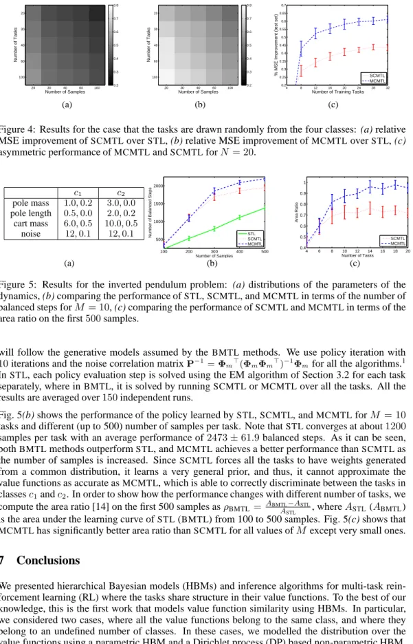
In the second experiment, we draw the tasks randomly from the four classes. We first applySCMTL
to this problem. Fig. 4(a) shows theSCMTL’s performance. As it can be seen, the results are worse than those in the first experiment (Fig. 3(c)), varying from30.15%±4.8 to54.05%±1.2. By clustering all the tasks together,SCMTLtakes advantage of all the available samples, thus, performs better thanSTL. However, when the tasks are drawn from significantly different distributions, it learns a very general prior which does not allow a significant improvement overSTL. We then apply
MCMTLto this problem. MCMTL’s performance (Fig. 4(b)) is significantly better thanSCMTL’s (Fig. 4(a)), and it varies from45.64%±5.6to77.65%±0.8. In order to evaluate how wellMCMTL
classifies the tasks, we also compare its performance to a version ofMCMTL in which each task is assigned to the right class in advance. The difference between the two algorithms is statistically significant only forN = 20(with the maximum of5.08%forM = 20), in which the noise on the samples makes it more difficult to discriminate between the distributions generating the tasks, and thus, to classify them correctly.
Finally, we compare the performance ofSCMTLandMCMTLin the asymmetric setting. At the end of each run of the symmetric problem, we draw100new test tasks at random from the same four classes used to generate the training tasks. We run the asymmetric algorithm described in Section 4.3 on each of the test tasks separately. Fig. 4(c) shows the performance ofSCMTLandMCMTLfor different number of training tasks andN fixed to20. The results indicate thatMCMTLperforms relatively better thanSCMTLas the number of training tasks increases.
6.2 Inverted Pendulum
The experiments of Section 6.1 indicate that when the tasks are generated exactly according to the generative models of Sections 3 and 4, the BMTLmethods can significantly improve the perfor-mance of a regression problem w.r.t. STL. As discussed in Section 2, the policy evaluation step of policy iteration can be casted as a regression problem, thus, similar improvement can be expected. In this section, we compare ourBMTLalgorithms withSTL in the problem of learning a control policy for balancing an inverted pendulum. Dynamics, reward function, and basis functions are the same as in [8]. Each task is generated by drawing the parameters of the dynamics (pole mass, pole length, cart mass, and noise on the actions) from Gaussian distributions with means and variances summarized in Fig. 5(a). The distribution over the two classes is uniform. It is worth noting that, unlike the regression experiments, here we have no guarantee that the weights of the value functions
Number of Samples Number of Tasks 20 30 40 60 100 20 30 40 60 100 0.2 0.3 0.4 0.5 0.6 0.7 0.8 (a) Number of Samples Number of Tasks 20 30 40 60 100 20 30 40 60 100 0.2 0.3 0.4 0.5 0.6 0.7 0.8 (b) 4 8 12 16 20 24 28 32 0.2 0.25 0.3 0.35 0.4 0.45 0.5 0.55 0.6 0.65 0.7
Number of Training Tasks
% MSE Improvement (test set) SCMTL MCMTL
(c)
Figure 4: Results for the case that the tasks are drawn randomly from the four classes: (a) relative MSE improvement ofSCMTLoverSTL, (b) relative MSE improvement ofMCMTLoverSTL, (c) asymmetric performance ofMCMTLandSCMTLforN= 20.
c1 c2 pole mass 1.0,0.2 3.0,0.0 pole length 0.5,0.0 2.0,0.2 cart mass 6.0,0.5 10.0,0.5 noise 12,0.1 12,0.1 100 200 300 400 500 500 1000 1500 2000 Number of Samples
Number of Balanced Steps STL
SCMTL MCMTL 4 6 8 10 12 14 16 18 20 0.4 0.5 0.6 0.7 0.8 0.9 1 Number of Tasks Area Ratio SCMTL MCMTL (a) (b) (c)
Figure 5: Results for the inverted pendulum problem: (a) distributions of the parameters of the dynamics, (b) comparing the performance ofSTL,SCMTL, andMCMTLin terms of the number of balanced steps forM = 10, (c) comparing the performance ofSCMTLandMCMTLin terms of the area ratio on the first500samples.
will follow the generative models assumed by the BMTLmethods. We use policy iteration with 10iterations and the noise correlation matrixP−1 =Φm⊤(ΦmΦm⊤)−
1
Φmfor all the algorithms.1
InSTL, each policy evaluation step is solved using the EM algorithm of Section 3.2 for each task separately, where inBMTL, it is solved by runningSCMTLorMCMTLover all the tasks. All the results are averaged over150independent runs.
Fig. 5(b) shows the performance of the policy learned bySTL,SCMTL, andMCMTLforM = 10 tasks and different (up to 500) number of samples per task. Note thatSTLconverges at about1200 samples per task with an average performance of2473±61.9balanced steps. As it can be seen, bothBMTLmethods outperformSTL, andMCMTLachieves a better performance thanSCMTLas the number of samples is increased. SinceSCMTLforces all the tasks to have weights generated from a common distribution, it learns a very general prior, and thus, it cannot approximate the value functions as accurate asMCMTL, which is able to correctly discriminate between the tasks in classesc1andc2. In order to show how the performance changes with different number of tasks, we
compute the area ratio [14] on the first 500 samples asρBMTL = ABMTL
−ASTL
ASTL , whereASTL (ABMTL)
is the area under the learning curve ofSTL(BMTL) from 100 to 500 samples. Fig. 5(c) shows that
MCMTLhas significantly better area ratio thanSCMTLfor all values ofM except very small ones.
7
Conclusions
We presented hierarchical Bayesian models (HBMs) and inference algorithms for multi-task rein-forcement learning (RL) where the tasks share structure in their value functions. To the best of our knowledge, this is the first work that models value function similarity using HBMs. In particular, we considered two cases, where all the value functions belong to the same class, and where they belong to an undefined number of classes. In these cases, we modelled the distribution over the value functions using a parametric HBM and a Dirichlet process (DP) based non-parametric HBM,
1
respectively. For each case, we derived inference algorithms for learning the value functions jointly and to transfer the knowledge acquired in the joint learning to improve the performance of learning the value function of a new task.
We first applied our proposed Bayesian multi-task learning (BMTL) algorithms to a regression prob-lem, in which the tasks are drawn from the generative models used by the BMTLmethods. The results indicate that BMTLalgorithms achieve significant improvement over single-task learning (STL) in both symmetric and asymmetric settings. We then applied our BMTLalgorithms to a benchmark RL problem, inverted pendulum. Although the tasks are no longer generated according to the models used by theBMTLalgorithms, they still outperformSTL. In our DP-based model we used Gibbs sampling, the most common simulation tool for Bayesian inference. We plan to look into variational techniques for Bayesian inference as an alternative approach.
8
Appendix
8.1 Details of the Single-class Multi-task Model
• Rm p(Rm|wm, θ) =p(Rm|wm, σ2) =N(HΦ⊤mnwm, σ2P) • wm p(wm|θ) =p(wm|µ,Σ) =N(µ,Σ) = (2π)−d/2|Σ|−1/2exp −1 2(wm−µ) ⊤ Σ−1(wm−µ) • θ p(θ|ψ0) =p(µ,Σ;µ0, k0, ν0,Σ0) × p(σ2;α0, β0) =N(µ;µ0,Σ/k0)IW(Σ;ν0,Σ0) × IG(σ2;α0, β0) = (2π/k0)−d/2|Σ|−1/2exp −k0 2 (µ−µ0) ⊤ Σ−1(µ−µ0) (normal) ×B|Σ0|ν0/2|Σ|−(ν0+d+1)/2exp −1 2tr Σ0Σ −1 (inverse-Wishart) × β α0 0 Γ(α0) 1 σ2 α0+1 exp −β0 σ2 (inverse-Gamma) where B−1= 2ν0d/2πd(d−1)/4 d Y j=1 Γ ν0+ 1−j 2 .
8.2 Posterior Distribution of the Parameters with the Normal-Inverse-Wishart×
Inverse-Gamma Prior
Taking advantage of the conjugate prior the posterior distribution overθ= (µ,Σ, σ2)given obser-vations{(wm, Rm)}M m=1and hyperpriorψ0is p(µ,Σ, σ2|wm, Rm, ψ0) =N(µ;µ′ 0,Σ/k ′ 0)IW(Σ;ν ′ 0,Σ ′ 0)× IG(σ2;α ′ 0, β ′ 0) (6)
where the posterior hyper-parametersψ′ 0= (µ ′ 0, k ′ 0, ν ′ 0,Σ ′ 0, α ′ 0, β ′ 0)are µ′0 = M k0+M ¯ w+ k0µ0 k0+M , (7) k′ 0 = k0+M , (8) ν′ 0 = ν0+M , (9) Σ′0 = Σ0+Q0+ k0M k0+M−m,c ( ¯w−µ0)( ¯w−µ0)⊤, (10) α′ 0 = α0+ N M 2 , (11) β′0 = β0+1 2 M X m=1 (HΦ⊤mwm−Rm) ⊤ P−1(HΦ⊤mwm−Rm), (12) wherew¯ = 1 M PM m=1wm,Q0=PMm=1(wm−w¯)(wm−w¯) ⊤ . 8.3 Gibbs Sampling
In this section, we report the equations used in the Gibbs sampling described in Section 4.2 of the paper. At each iteration of the MCMTL algorithm of Figure 2 in the paper, the Gibbs sampling is fed with observations({wbm},{Rm}), wherewbm=µ′
0m. In particular, we use the the Gibbs sampling
with conjugate-priors (Algorithm 3 in [12]).
We begin with the probability of taskmbelonging to a new class. Given observation(wbm, Rm)and hyper-priorψ0, the non-normalized probability can be written as
Z p(Rm,wm|θ)p(θ|ψ0)dθ= k0 πk′ 0 d/2 |Σ0|ν0/2 |Σ′0|ν′ 0/2 Γν0′ 2 Γν0′−d 2 ×(2π|P|)−N/2 β α0 0 Γ(α0) Γ(α′ 0) β′α′0 0 , where hyper-parametersψ′ 0= (µ ′ 0, k ′ 0, ν ′ 0,Σ ′ 0, α ′ 0, β ′
0)are computed as in Section 8.2 for
observa-tion(Rm,wm).
Similarly, letm′:c
m′ =c, m′6=m, then the posterior over parameters for classcis
p(µc,Σc, σ2
c|{wbm′},{Rm′}, ψ0) =N(µc;µ0c,Σc/k0)IW(Σc;ν0c,Σ0c)× IG(σ2c;α0c, β0c)(13)
with the following posterior hyper-parameters (which play the role of prior hyper-parameters for the class) µ0c = M−m,c k0+M−m,c ¯ w+ k0µ0 k0+M−m,c , (14) k0c = k0+M−m,c, (15) ν0c = ν0+M−m,c, (16) Σ0c = Σ0+Q0+ k0M−m,c k0+M−m,c ( ¯w−µ0)( ¯w−µ0)⊤, (17) α0c = α0+N M −m,c 2 , (18) β0c = β0+1 2 X m′ (HΦ⊤ mwbm−Rm) ⊤ P−1(HΦ⊤ mwbm−Rm), (19)
whereM−m,cis the number of tasks belonging to classcexcept taskm,w¯ = M1 −m,c
P
m′wbm′, and
Q0 =Pm′(wbm′ −w¯)(wbm′−w¯) ⊤
. As a result, the integral for the probability of taskmbelong to classcbecomes
Z p Rm,wbm|θp θ|{cm′}, ψ0dθ= Z p Rm,wbm|θp θ|ψ0cdθ = k0c πk′ 0c d/2 |Σ0c|ν0c/2 |Σ′ 0c|ν ′ 0c/2 Γν0′c 2 Γν0′c−d 2 ×(2π|P|)−N/2 β α0c 0c Γ(α0c) Γ(α′ 0c) β′α′0c 0 , whereψ′
0cis computed as in Equations (2)-(7) but usingψ0cas prior instead ofψ0.
8.4 Noise Correlation Models
We analyze the equations forwbmfor two different noise correlation models. In particular we show that depending on the covariance matrix, both GPTD and BMTL can be seen as extensions of either Bellman residual minimization (BRM) or LSTD.
We first analyze the general formulation withS=σ2Pbe the covariance matrix of the noise. Letθ= (µ,Σ, σ2)be the model parameters. The expected value of the weights in BMTL is written as b wm= 1 σ2ΦmH ⊤ P−1HΦ⊤m+Σ−1 −1 1 σ2ΦmH ⊤ P−1Rm+Σ−1µ , (20)
whereS = σ2Pis the noise covariance matrix modeling the correlation of the noise at different states. We callσ2andPthe noise variance and the noise correlation matrix, respectively.
In caseµ =0 andΣ =I, we obtain a general form for the posterior mean of the weights in the parametric form of GPTD (Equation (4.4.41) in [5])
b
wm=hΦmH⊤P−1HΦ⊤m+σ2Ii
−1
ΦmH⊤P−1Rm. (21)
The (parametric) GPTD of [5; 6] is obtained by settingP = HH⊤ in Equation (21). As it was
shown in Section 4.5 of [5], by settingσ2→0andP−1=Φ
m ⊤
GΦmin Equation (21), whereGis an arbitraryd×dsymmetric positive-definite matrix, we can derive a new set of GPTD algorithms that are based on the LSTD(0) algorithm. As it was discussed in Section 4.5.3 of [5], a reasonable choice forGisG=ΦmΦm⊤
−1
.
8.5 Experiment Setups
In the following we list all the details about the setup used in the experiments of the paper. We report the hyper-prior parameters(τ, ψ0)and the parameters used in the inference algorithm. In particular,
ǫEM is the threshold used in the stopping condition of the EM algorithm,nMCMTL is the maximum
number of iterations of the outer loop ofMCMTL, andnGibbsis the number of steps of the Gibbs
sampling. In none of the experiments the parameters have been systematically optimized.
8.5.1 The Regression Problem
In Figure 6 we report examples of the functions (tasks) and the generated samples for each of the four different classes used in the experiments of Section 6.1 of the paper. The parameters used in the ex-periments are reported in Tables 1. As it can be noticed the prior is not very informative and it has not been optimized for this specific problem. Since the four classes are quite well separated, the value of the concentrationτis not critical for the success of theMCMTLalgorithm. Finally, the length of the Gibbs sampling changes with the number of tasks, so that when many tasks are involved, a longer MCMC simulation is performed and a more accurate estimation ofp({cm}|{wbm},{Rm}, τ, ψ0)is
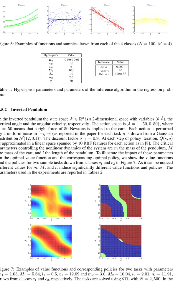
−1 −0.5 0 0.5 1 30 40 50 60 70 80 x C lassc1 −1 −0.5 0 0.5 1 −3 −2 −1 0 1 2 3 x C lassc2 −1 −0.5 0 0.5 1 −20 −10 0 10 20 x C lassc3 −1 −0.5 0 0.5 1 −80 −70 −60 −50 −40 −30 −20 x C lassc4
Figure 6: Examples of functions and samples drawn from each of the4classes (N = 100,M = 4).
Hyper-prior Value µ0 [0 0 0 0 0 0] k0 1.0 ν0 6 Σ0 10I β0 1.0 α0 2.0 τ 30 Inference Value ǫEM 0.0001 nMCMTL 10 nGibbs 100×M
Table 1: Hyper-prior parameters and parameters of the inference algorithm in the regression prob-lem.
8.5.2 Inverted Pendulum
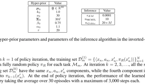
In the inverted pendulum the state spaceX ∈R2is a 2-dimensional space with variables(θ,θ˙), the vertical angle and the angular velocity, respectively. The action space isA={−50,0,50}, where a = 50means that a right force of50Newtons is applied to the cart. Each action is perturbed by a uniform noise in[−η, η](as reported in the paper for each taskη is drawn from a Gaussian distributionN(12,0.1)). The discount factor isγ = 0.9. At each step of policy iteration,Q(s, a) is approximated in a linear space spanned by 10 RBF features for each action as in [8]. The critical parameters controlling the nonlinear dynamics of the system aremthe mass of the pendulum,M the mass of the cart, andlthe length of the pendulum. To illustrate the impact of these parameters on the optimal value function and the corresponding optimal policy, we show the value functions and the policies for two sample tasks drawn from classesc1andc2in Figure 7. As it can be noticed
different values form,M, andl, induce significantly different value functions and policies. The parameters used in the experiments are reported in Tables 2.
−1.5 −1 −0.5 0 0.5 1 1.5 −2 −1.5 −1 −0.5 0 0.5 1 1.5 2 θ ˙θ −1.5 −1 −0.5 0 0.5 1 1.5 −2 −1.5 −1 −0.5 0 0.5 1 1.5 2 θ ˙θ −1.5 −1 −0.5 0 0.5 1 1.5 −2 −1.5 −1 −0.5 0 0.5 1 1.5 2 θ ˙θ −1.5 −1 −0.5 0 0.5 1 1.5 −2 −1.5 −1 −0.5 0 0.5 1 1.5 2 θ ˙θ
Figure 7: Examples of value functions and corresponding policies for two tasks with parameters m1= 1.03,M1= 5.64,l1= 0.5,η1= 12.09andm2= 3.0,M2= 10.04,l2= 2.01,η2= 11.91,
drawn from classesc1andc2, respectively. The tasks are solved usingSTLwithN = 2,500. In the
Hyper-prior Value µ0 0∈R 30 k0 1.0 ν0 30 Σ0 30I β0 0.75 α0 1.1 τ 20 Inference Value ǫEM 0.0001 nMCMTL 10 nGibbs 20×M
Table 2: Hyper-prior parameters and parameters of the inference algorithm in the inverted-pendulum problem.
At iterationk= 1of policy iteration, the training setD(1)m ={hxn, an, x′n, πR(x′n)i}Nn=1is built by
following a fully random policyπRfor each taskMm. At iterationk= 2,3, . . ., all the samples in
the training setD(mk)have the samexn, an, x′ncomponents, while the fourth component is changed
according to πk−1(x′n). At the end of policy iteration, the performance of the learned policy is
evaluated by taking the average over 30 episodes with a maximum of 3,000 steps each.
References
[1] J. Baxter. A model of inductive bias learning. Journal of Artificial Intelligence Research, 12: 149–198, 2000.
[2] D. Bertsekas and J. Tsitsiklis. Neuro-Dynamic Programming. Athena Scientific, 1996. [3] E. Bonilla, K. Chai, and C. Williams. Multi-task Gaussian process prediction. In Proceedings
of NIPS 20, pages 153–160, 2008.
[4] R. Caruana. Multitask learning. Machine Learning, 28(1):41–75, 1997.
[5] Y. Engel. Algorithms and Representations for Reinforcement Learning. PhD thesis, The He-brew University of Jerusalem, Israel, 2005.
[6] Y. Engel, S. Mannor, and R. Meir. Reinforcement learning with Gaussian processes. In
Pro-ceedings of ICML 22, pages 201–208, 2005.
[7] H. Ishwaran and L. James. Gibbs sampling methods for stick-breaking priors. Journal of the
American Statistical Association, 96:161–173, 2001.
[8] M. Lagoudakis and R. Parr. Least-squares policy iteration. JMLR, 4:1107–1149, 2003. [9] A. Lazaric, M. Restelli, and A. Bonarini. Transfer of samples in batch reinforcement learning.
In Proceedings of ICML 25, pages 544–551, 2008.
[10] N. Mehta, S. Natarajan, P. Tadepalli, and A. Fern. Transfer in variable-reward hierarchical reinforcement learning. Machine Learning, 73(3):289–312, 2008.
[11] S. Mukhopadhyay and A. Gelfand. Dirichlet process mixed generalized linear models. Journal
of the American Statistical Association, 92(438):633–639, 1997.
[12] R. Neal. Markov chain sampling methods for Dirichlet process mixture models. Journal of
Computational and Graphical Statistics, 9(2):249–265, 2000.
[13] R. Sutton and A. Barto. An Introduction to Reinforcement Learning. MIT Press, 1998. [14] M. Taylor, P. Stone, and Y. Liu. Transfer learning via inter-task mappings for temporal
differ-ence learning. JMLR, 8:2125–2167, 2007.
[15] A. Wilson, A. Fern, S. Ray, and P. Tadepalli. Multi-task reinforcement learning: A hierarchical Bayesian approach. In Proceedings of ICML 24, pages 1015–1022, 2007.
[16] Y. Xue, X. Liao, L. Carin, and B. Krishnapuram. Multi-task learning for classication with dirichlet process priors. JMLR, 8:35–63, 2007.
[17] K. Yu, V. Tresp, and A. Schwaighofer. Learning Gaussian processes from multiple tasks. In