Matrix adaptation in discriminative vector quantization

(1)

Matrix adaptation in discriminative

vector quantization

Petra Schneider

1 , Michael Biehl

1 , Barbara Hammer

2 IfI Technical Report Series

IFI-08-08

(2)

Impressum

Publisher: Institut für Informatik, Technische Universität Clausthal

Julius-Albert Str. 4, 38678 Clausthal-Zellerfeld, Germany

Editor of the series: Jürgen Dix Technical editor: Wojciech Jamroga Contact: [email protected]

URL: http://www.in.tu-clausthal.de/forschung/technical-reports/

ISSN: 1860-8477

The IfI Review Board

Prof. Dr. Jürgen Dix (Theoretical Computer Science/Computational Intelligence) Prof. Dr. Klaus Ecker (Applied Computer Science)

Prof. Dr. Barbara Hammer (Theoretical Foundations of Computer Science) Prof. Dr. Sven Hartmann (Databases and Information Systems)

Prof. Dr. Kai Hormann (Computer Graphics)

Prof. Dr. Gerhard R. Joubert (Practical Computer Science) apl. Prof. Dr. Günter Kemnitz (Hardware and Robotics) Prof. Dr. Ingbert Kupka (Theoretical Computer Science)

Prof. Dr. Wilfried Lex (Mathematical Foundations of Computer Science) Prof. Dr. Jörg Müller (Business Information Technology)

Prof. Dr. Niels Pinkwart (Business Information Technology) Prof. Dr. Andreas Rausch (Software Systems Engineering) apl. Prof. Dr. Matthias Reuter (Modeling and Simulation) Prof. Dr. Harald Richter (Technical Computer Science) Prof. Dr. Gabriel Zachmann (Computer Graphics)

(3)

Petra Schneider1, Michael Biehl1, Barbara Hammer2

1_{Institute for Mathematics and Computing Science, University of Groningen}

P.O. Box 407, 9700 AK Groningen, The Netherlands

{p.schneider,m.biehl}@rug.nl

2_{Institute of Computing Science, Clausthal University of Technology}

Julius Albert Strasse 4, 38678 Clausthal - Zellerfeld, Germany

[email protected]

Abstract

Discriminative vector quantization schemes such as learning vector quantization (LVQ) and extensions thereof offer efficient and intuitive classifiers which are based on the representation of classes by prototypes. The original methods, however, rely on the Euclidean distance corresponding to the assumption that the data can be represented by isotropic clusters. For this reason, extensions of the methods to more general metric structures have been proposed such as relevance adaptation in generalized LVQ (GLVQ) and matrix learning in GLVQ. In these approaches, metric parameters are learned based on the given classification task such that a data driven distance measure is found. In this article, we consider full matrix adaptation in advanced LVQ schemes; in particular, we introduce matrix learning to a recent statistical formalization of LVQ, robust soft LVQ, and we compare the results on several artificial and real life data sets to matrix learning in GLVQ, which consti-tutes a derivation of LVQ-like learning based on a (heuristic) cost function. In all cases, matrix adaptation allows a significant improvement of the classification ac-curacy. Interestingly, however, the principled behavior of the models with respect to prototype locations and extracted matrix dimensions shows several characteristic differences depending on the data sets.

Keywords: learning vector quantization, generalized LVQ, robust soft LVQ, metric

adaptation

1 Introduction

Discriminative vector quantization schemes such as learning vector quantization (LVQ) constitute very popular classification methods due to their intuitivity and robustness: they represent the classification by (usually few) prototypes which constitute typical representatives of the respective classes and, thus, allow a direct inspection of the given classifier. Training often takes place by Hebbian learning such that very fast and simple

(4)

Introduction

training algorithms result. Further, unlike the perceptron or the support vector machine, LVQ provides an integrated and intuitive classification model for any given number of classes. Numerous modifications of original LVQ exist which extend the basic learning scheme as proposed by Kohonen towards adaptive learning rates, faster convergence, or better approximation of Bayes optimal classification, to name just a few [ 8]. Despite their popularity and efficiency, most LVQ schemes are solely based on heuristics and a deeper mathematical investigation of the models has just recently been initiated. On the one hand, their worst case generalization capability can be limited in terms of gen-eral margin bounds using techniques from computational learning theory [ 5, 4]. On the other hand, the characteristic behavior and learning curves of popular models can ex-actly be investigated in typical model situations using the theory of online learning [ 2]. Many questions, however, remain unsolved such as convergence and typical prototype locations of heuristic LVQ schemes in concrete, finite training settings.

Against this background, researchers have proposed variants of LVQ which can di-rectly be derived from an underlying cost function which is optimized during train-ing e.g. by means of a stochastic gradient ascent/descent. Generalized LVQ (GLVQ) as proposed by Sato and Yamada constitutes one example [ 10]: its intuitive (though heuristic) cost function can be related to a minimization of classification errors and, at the same time, a maximization of the hypothesis margin of the classifier which charac-terizes its generalization ability [5]. The resulting algorithm is indeed very robust and powerful, however, an exact mathematical analysis is still lacking. A very elegant and mathematically well-founded alternative has been proposed by Seo and Obermayer: in [12], a statistical approach is introduced which models given classes as mixtures of Gaussians. Prototype parameters are optimized by maximizing the likelihood ratio of correct versus incorrect classification. A learning scheme which closely resembles LVQ2.1 results. This cost function, however, is unbounded such that numerical insta-bilities occur which, in practice, cause the necessity of restricting updates to data from a window close to the decision boundary. The approach of [ 12] offers an elegant alter-native: A robust optimization scheme is derived from a maximization of the likelihood ratio of the probability of correct classification versus the total probability in a Gaus-sian mixture model. The resulting learning scheme, robust soft LVQ (RSLVQ), leads to an alternative discrete LVQ scheme where prototypes are adapted solely based on misclassifications.

RSLVQ constitutes a very attractive model due to the fact that all underlying model assumptions are stated explicitly in the statistical formulation – and, they can easily be changed if required by the application scenario. Besides, the resulting model shows superior classification accuracy compared to GLVQ in a variety of settings as we will demonstrate in this article.

All these methods, however, suffer from the problem that classification is based on a predefined metric. The use of Euclidean distance, for instance, corresponds to the implicit assumption of isotropic clusters. Such models can only be successful if the data displays a Euclidean characteristic. This is particularly problematic for high-dimensional data where noise accumulates and disrupts the classification, or hetero-geneous data sets where different scaling and correlations of the dimensions can be

(5)

observed. Thus, a more general metric structure would be beneficial in such cases. The field of metric adaptation constitutes a very active research topic in various distance based approaches such as unsupervised or semi-supervised clustering and visualization

[1, 7],_k-nearest neighbor approaches [ 14, 15] and learning vector quantization [ 6, 11].

We will focus on matrix learning in LVQ schemes which accounts for pairwise corre-lations of features, i.e. a very general and flexible set of classifiers. On the one hand, we will investigate the behavior of generalized matrix LVQ (GMLVQ) in detail, a ma-trix adaptation scheme for GLVQ which is based on a heuristic, though intuitive cost function. On the other hand, we will develop matrix adaptation for RSLVQ, a statistical model for LVQ schemes, and thus we will arrive at a uniform statistical formulation for prototype and metric adaptation in discriminative prototype-based classifiers. We will introduce variants which adapt the matrix parameters globally based on the training set or locally for every given prototype or mixture component, respectively.

Matrix learning in RSLVQ and GLVQ will be evaluated and compared in a variety of learning scenarios: first, we consider test scenarios where prior knowledge about the form of the data is available. Furthermore, we compare the methods on several benchmarks from the UCI repository [ 9].

Interestingly, depending on the data, the methods show different characteristic be-havior with respect to prototype locations and learned metrics. Although the classifica-tion accuracy is in many cases comparable, they display quite different behavior con-cerning their robustness with respect to parameter choices and the characteristics of the solutions. We will point out that these findings have consequences on the interpretabil-ity of the results. In all cases, however, matrix adaptation leads to an improvement of the classification accuracy, despite a largely increased number of free parameters.

2 Advanced learning vector quantization schemes

Learning vector quantization has been introduced by Kohonen [ 8], and a variety of extensions and generalizations exist. Here we focus on approaches based on a cost function, i.e. generalized learning vector quantization (GLVQ) and robust soft learning vector quantization (RSLVQ).

Assume training data{ξ_i, yi}li=1 ∈ RN × {1, . . . , C} are given,N denoting the

data dimensionality and_C the number of different classes. An LVQ network_W =

{(w_j, c(w_j)) : RN× {1, . . . , C}}m_j₌₁consists of a number_mof prototypesw∈RN

which are characterized by their location in feature space and their class label_c(w)∈

{1. . . , C}. Classification is based on a winner takes all scheme. A data pointξ∈RN

is mapped to the label_c(ξ) =c(w_i)of the prototype, for which_d(ξ,wi)≤d(ξ,wj)

holds∀_j =i. Here_dis an appropriate distance measure. Hence,ξis mapped to the

class of the closest prototype, the so-called winner. Often,_dis chosen as the squared

Euclidean metric, i.e._d(ξ,w) = (ξ−w)T(ξ−w).

LVQ algorithms aim at an adaptation of the prototypes such that a given data set is classified as accurately as possible. The first LVQ schemes proposed heuristic adap-tation rules based on the principle of Hebbian learning, such as LVQ2.1, which, for

(6)

Advanced learning vector quantization schemes

a given data pointξ, adapts the closest prototype w+(ξ) with the same class label

c(w+(ξ)) =c(ξ)into the direction ofξ: Δw+(ξ) =α·(ξ−w+(ξ))and the

clos-est incorrect prototypew−(ξ)with a different class label_c(w−(ξ))=c(ξ)is moved

into the opposite direction:Δw− =−α·(ξ−w−(ξ)). Here,_{α >}0is the learning

rate. Since, often, LVQ2.1 shows divergent behavior, a window rule is introduced, and

adaptation takes place only ifw+(ξ)andw−(ξ)are the closest two prototypes ofξ.

Generalized LVQ derives a similar update rule from the following cost function:

EGLVQ= l i=1 Φ(μ(ξ_i)) = l i=1 Φ d(ξ_i,w+(ξ_i))−d(ξ_i,w−(ξ_i)) d(ξ_i,w+(ξ_i)) +d(ξ_i,w−(ξ_i)) . (1)

Φis a monotonic function such as the logistic function or the identity which is used

throughout the following. The numerator of a single summand is negative if the

classi-fication ofξis correct. Further, a small value corresponds to a classification with large

margin, i.e. large difference of the distance to the closest correct and incorrect proto-type. In this sense, GLVQ tries to minimize the number of misclassifications and to maximize the margin of the classification. The denominator accounts for a scaling of

the terms such that the arguments ofΦare restricted to the interval(−1,1)and

numer-ical problems are avoided. The cost function of GLVQ can be related to a compromise of the minimization of the training error and the generalization ability of the classifier which is determined by the hypothesis margin (see [ 4, 5]). The connection, however, is not exact. The update formulas of GLVQ can be derived by means of the gradients of

EGLVQ(see [10]). Interestingly, the learning rule resembles LVQ2.1 in the sense that

the closest correct prototype is moved towards the considered data point and the closest incorrect prototype is moved away from the data point. The size of this adaptation step

is determined by the magnitude of terms stemming from_E_GLVQ; this change accounts

for a better robustness of the algorithm compared to LVQ2.1.

Unlike GLVQ, robust soft learning vector quantization is based on a statistical mod-elling of the situation which makes all assumptions explicit: the probability density of

the underlying data distribution is described by a mixture model. Every component_j

of the mixture is assumed to generate data which belongs to only one of the_Cclasses.

The probability density of the full data set is given by

p(ξ|W) = C i=1 m j:c(wj)=i p(ξ|j)P(j), (2)

where the conditional density_p(ξ|j)is a function of prototypew_j. For example, the

conditional density can be chosen to have the normalized exponential formp(ξ|j) =

K(j)·expf(ξ,wj, σj2), and the priorP(j)can be chosen identical for every prototype

wj. RSLVQ aims at a maximization of the likelihood ratio:

ERSLVQ= l i=1 log p(ξ_i, yi|W) p(ξ_i|W) , (3)

(7)

where_p(ξ_i, yi|W)is the probability density thatξi is generated by a mixture

compo-nent of the correct class_y_i and_p(ξ_i|W) is the total probability density ofξ_i. This

implies p(ξ_i, yi|W) = j:c(wj)=yi p(ξ_i|j)P(j), p(ξ_i|W) = j p(ξ_i|j)P(j). (4)

The learning rule of RSLVQ is derived from_E_RSLVQ by a stochastic gradient ascent.

Since the value of_E_RSLVQdepends on the position of all prototypes, the complete set

of prototypes is updated in each learning step. The gradient of a summand of_E_RSLVQ

for data point(ξ, y)with respect to a prototypew_jis given by (see the appendix)

where the Kronecker symbol_δ_y,c₍_w_j₎tests whether the labels_yand_c(w_j)coincide. In

the special case of a Gaussian mixture model with_σ_j2=σ2and_P(j) = 1/mfor all_j,

we obtain

f(ξ,w, σ2) = −d(ξ,w)

2σ2 , (6)

where_d(ξ,w)is the distance measure between data pointξand prototypew. Original

RSLVQ is based on the squared Euclidean distance. This implies

f(ξ,w, σ2) =−(ξ−w) T₍_ξ₋_w₎ 2σ2 , ∂f ∂w = 1 σ2(ξ−w). (7)

Substituting the derivative of_f in equation ( 5) yields the update rule for the prototypes

in RSLVQ Δw_j= α1 σ2 (Py(j|ξ)−P(j|ξ))(ξ−wj), c(wj) =y, −P(j|ξ)(ξ−w_j), c(w_j)=y, (8)

where_α₁ _>0is the learning rate. In the limit of vanishing softness_σ2, the learning

rule reduces to an intuitive crisp learning from mistakes (LFM) scheme, as pointed out in [12]: in case of erroneous classification, the closest correct and the closest wrong prototype are adapted along the direction pointing to / from the considered data point. Thus, a learning scheme very similar to LVQ2.1 results which reduces adaptation to wrongly classified inputs close to the decision boundary. While the soft version as introduced in [12] leads to a good classification accuracy as we will see in experiments, the limit rule has some principled deficiencies as shown in [ 2].

(8)

Matrix learning in advanced LVQ schemes

3 Matrix learning in advanced LVQ schemes

The squared Euclidean distance gives rise to isotropic clusters, hence the metric is not appropriate if data dimensions show a different scaling or correlations. A more general form can be obtained by extending the metric by a full matrix

dΛ(ξ,w) = (ξ−w)TΛ(ξ−w), (9)

whereΛis an_N×_N-matrix which is restricted to positive definite forms to guarantee

metricity. We can achieve this by substitutingΛ = ΩTΩ, whereΩ∈RM×N. Further,

Λhas to be normalized after each learning step to prevent the algorithm from

degen-eration. Two possible approaches are to restrict_iΛ_iiordet(Λ)to a fixed value, i.e.

either the sum of eigenvalues or the product of eigenvalues is constant. Note that

nor-malizingdet(Λ)requires_M ≥_N, since otherwiseΛwould be singular. In this work,

we always set_M =N. Since an optimal matrix is not known beforehand for a given

classification task, we adaptΛorΩ, respectively, during training. For this purpose, we

substitute the distance in the cost functions of LVQ by the new measure

dΛ(ξ,w) =

i,j,k

(ξi−wi)ΩkiΩkj(ξj−wj). (10) Generalized matrix LVQ (GMLVQ) extends the cost function_E_GLVQby this more

general metric and adapts the matrix parametersΩ_ij together with the prototypes by

means of a stochastic gradient descent. The derivatives

∂dΛ(ξ,w) ∂w =−2Λ(ξ−w), ∂dΛ(ξ,w) ∂Ω_lm = 2 i (ξi−wi)Ωli(ξm−wm)

yield the GMLVQ update rules

Δw+=α1·Φ(μ(ξ))·μ+(ξ)·Λ·dΛ(ξ,w+(ξ)), (11) Δw− =−α1·Φ(μ(ξ))·μ−(ξ)·Λ·dΛ(ξ,w−(ξ)), (12) ΔΩ_lm =−α2·Φ(μ(ξ))· μ+(ξ)· [Ω(ξ−w+(ξ))]l(ξm−w+m) −μ−(ξ)· [Ω(ξ−w−(ξ))]l(ξm−w−m) , (13)

where_α₂_>0is the learning rate for the metric parameter and_μ+(ξ) =d(ξ,w−(ξ))/

(d(ξ,w+(ξ))+d(ξ,w−(ξ)))2, μ−(ξ) =d(ξ,w+(ξ))/(d(ξ,w−(ξ))+d(ξ,w−(ξ)))2.

It is possible to introduce one global matrixΩ, which corresponds to a global

(9)

every prototype. The latter corresponds to the possibility to adapt individual ellipsoidal clusters around every prototype. In this case, the squared distance is computed by

d(ξ,wj) = (ξ−wj)TΛj(ξ−wj). (14) Using this approach, the updates for the prototypes (Eq.s 12,13) include the local

ma-tricesΛ+, Λ−. For the metric parameters, the learning rules constitute

ΔΩ+_lm=−α2·Φ(μ(ξ))·μ+(ξ)· [Ω+(ξ−w+(ξ))]_l(ξm−wm+) , (15) ΔΩ−_lm=α2·Φ(μ(ξ))·μ−(ξ)· [Ω−(ξ−w−(ξ))]_l(ξm−w−m) . (16)

We refer to the extension of GMLVQ with local relevance matrices by the term local

GMLVQ (LGMLVQ).

Now, we extend RSLVQ by the more general metric introduced in equation ( 9). The

conditional density function obtains the form_p(ξ|j) =K(j)·expf(ξ,w, σ2,Ω)with

f(ξ,w, σ2,Ω) = −(ξ−w) T_ΩT_Ω(_ξ₋_w₎ 2σ2 , (17) ∂f ∂w = 1 σ2Ω T_{Ω (}_ξ₋_w_{) =} 1 σ2Λ (ξ−w), (18) ∂f ∂Ω_lm =− 1 σ2 i (ξi−wi)Ωli(ξm−wm) . (19)

Combining equations (5) and (18) yields the new update rule for the prototypes:

Δw_j= α1

σ2

(Py(j|ξ)−P(j|ξ)) Λ (ξ−wj), c(wj) =y,

−P(j|ξ) Λ (ξ−w_j), c(w_j)=y. (20)

Taking the derivative of the summand_E_RSLVQfor training sample(ξ, y)with respect

to a matrix elementΩlmleads us to the update rule (see the appendix)

ΔΩlm=− α2 σ2 · j δy,c(wj)(Py(j|ξ)−P(j|ξ))−(1−δy,c(wj))P(j|ξ) · [Ω(ξ−w_j)]_l(ξm−wj,m) , (21)

where_α₂ _>0is the learning rate for the metric parameters. The algorithm based on

(10)

Matrix learning in advanced LVQ schemes

the following. Similar to local matrix learning in GMLVQ, it is also possible to train an

individual matrixΛ_j for every prototype. With individual matrices attached to all

pro-totypes, the modification of (20) which includes the local matricesΛ_jis accompanied

by (see the appendix)

ΔΩj,lm=−α2 σ2 · δy,c(wj)(Py(j|ξ)−P(j|ξ))−(1−δy,c(wj))P(j|ξ) · [Ωj(ξ−wj)]l(ξm−wj,m) , (22)

under the constraint_K(j) =const.for all_j. We term this learning rule local MRSLVQ

(LMRSLVQ). Due to the restriction to constant normalization factorsK(j), the

normal-izationdet(Λ_j) =const.is assumed for this algorithm. Note that under the assumption

of equal priorsP(j), a classifier using one prototype per class is still given by the

stan-dard LVQ classifier: ξ→ _c(w_j)for which_d_Λ_j(ξ,wj)is minimum. In more general

settings, nearest prototype classification should coincide with the class of maximum likelihood ratio for most inputs since prototypes are usually distant from each other

compared to the bandwidth_σ2. Interestingly, the generalization ability of this function

class has been investigated in [11] including the possibility of adaptive local matrices. Worst case generalization bounds which depend on the number of prototypes and the hypothesis margin, i.e. the minimum difference between the closest correct and wrong prototype, can be found which are independent of the input dimensionality (in particu-lar independent of the matrix dimensionality), such that good generalization capability can be expected from these classifiers. We will investigate this claim in several exper-iments. In addition, we will have a look at the robustness of the methods with respect to hyperparameters, the interpretability of the results, and the uniqueness of the learned matrices.

Although GLVQ and RSLVQ constitute two of the most promising theoretical deriva-tions of LVQ schemes from global cost funcderiva-tions, they have so far not been compared in experiments. Further, matrix learning offers a striking extension of RSLVQ since it extends the underlying Gaussian mixture model towards the general form of arbitrary covariance matrices, which has not been introduced or tested so far. Thus, we are inter-ested in several aspects and questions which should be highlighted by the experiments:

• What is the performance of the methods on real life data sets of different

charac-teristics? Can the theoretically motivated claim of good generalization ability be substantiated by experiments?

• What is the robustness of the methods with respect to metaparameters such as

σ2?

(11)

pro-totype location change due to the specific learning rule in a discriminative ap-proach?

• Are the extracted matrices meaningful? In how far do they differ between the

approaches?

• Do there exist systematic differences in the solutions found by RSLVQ and GLVQ

(with / without matrix adaptation)?

We first test the methods on two artificial data sets where the underlying density is known exactly, which are designed for the evaluation of matrix adaptation. Afterwards, we compare the algorithms on benchmarks from UCI [ 9].

4 Experiments

With respect to parameter initialization and learning rate annealing, we use the same strategies in all experiments. The mean values of random subsets of training samples selected from each class are chosen as initial states of the prototypes. The

hyperparame-ter_σ2is held constant in all experiments with RSLVQ, MRSLVQ and Local MRSLVQ.

The learning rates are continuously reduced in the course of learning. We implement a schedule of the form

αi(t) = αi

1 +c(t−1) (23)

(_i∈ {1,2}), where_tcounts the number training epochs. The factor_cdetermines the

speed of annealing and is chosen individually for every application. Special attention has to be paid to the normalization of the relevance matrices. With respect to the inter-pretability, it is advantageous to fix the sum of eigenvalues to a certain value. Besides, we observe that this approach shows a better performance and learning behaviour com-pared to the restriction of the matrices’ determinant. For this reason, the normalization

iΛii = 1is used for the applications in Sec. 4.1, since we do not discuss the

adap-tation of local matrices there. We initially setΛ = _N1 ·1, which results indΛ being

equivalent to the Euclidean distance. Note that, in consequence, the Euclidean distance in RSLVQ and GLVQ has to be normalized to one as well to allow for a fair com-parison with respect to learning rates. Accordingly, the RSLVQ- and GLVQ prototype

updates and the function_fin equation ( 7) have to be weighted by1/N.Training of local

MRSLVQ in Sec. 4.2 requires the normalizationdet(Λ_j) = 1. The local matricesΛ_j

are initialized by the identity matrix in this case.

4.1 Artificial Data

In the first experiments, the algorithms are applied to the artificial data from [ 3] to illus-trate the training of an LVQ-classifier based on the alternative cost functions with fixed and adaptive distance measure. The data sets 1 and 2 comprise three-class classification problems in a two dimensional space. Each class is split into two clusters with small or

(12)

Experiments

large overlap, respectively (see Figure 1). We randomly select 2/3 of the data samples of each class for training and use the remaining data for testing. According to the a pri-ori known distributions, the data is represented by two prototypes per class. Since we observe that the algorithms based on the RSLVQ cost function are very sensitive with respect to the learning parameter settings, slightly smaller values are chosen to train a classifier with (M)RSLVQ compared to G(M)LVQ. We use the settings

G(M)LVQ:_α₁= 5·10−3, α2= 1·10−3, c= 1·10−3

(M)RSLVQ:_α₁= 5·10−4, α2= 1·10−4, c= 1·10−3

and perform 1000 sweeps through the training set. The results presented in the follow-ing are averaged over 10 independent constellations of trainfollow-ing and test set. We apply

several different valuesσ2from the interval [0.001, 0.015] and present the simulations

giving rise to the best mean performance on the training sets.

The results are summarized in Table 1. They are obtained with the hyperparameters

settings_σ_opt2 (RSLVQ) = 0.002and_σ_opt2 (MRSLVQ) = 0.002,0.003for data set 1

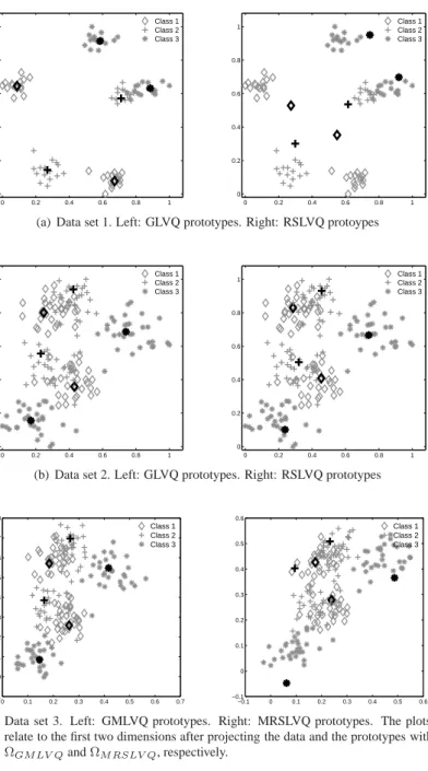
and 2, respectively. The use of the advanced distance measure yields only a slight im-provement compared to the fixed Euclidean distance, since the distributions do not have favorable directions to classify the data. On data set 1, GLVQ and RSLVQ show nearly the same performance. However, the prototype configurations identified by the two al-gorithms vary significantly (see Figure 1). During GLVQ-training, the prototypes move close to the cluster centers in only a few training epochs, resulting in an appropriate approximation of the data by the prototypes. On the contrary, prototypes are frequently located outside the clusters, when the classifier is trained with the RSLVQ-algorithm. This behavior is due to the fact that only data points lying close to the decision bound-ary change the prototype constellation in RSLVQ significantly (see equation ( 8)). As depicted in Figure 2, only a small number of training samples are lying in the active region of the prototypes while the great majority of training samples attains only tiny weight values in equation (8) which are not sufficent to adjust the prototypes to the data in reasonable training time. This effect does not have negative impact on the

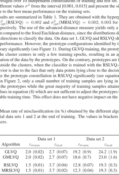
classifica-Table 1: Mean rate of misclassification (in %) obtained by the different algorithms on

the artificial data sets 1 and 2 at the end of training. The values in brackets constitute the variances.

Data set 1 Data set 2

Algorithm _ε_train _ε_test _ε_train _ε_test

GLVQ 2.0 (0.02) 2.7 (0.07) 19.2 (0.9) 24.2 (1.9)

GMLVQ 2.0 (0.02) 2.7 (0.07) 18.6 (0.7) 23.0 (1.6)

RSLVQ 1.5 (0.01) 3.7 (0.04) 12.8 (0.07) 19.3 (0.3)

(13)

tion of the data set. However, the prototypes do not provide a reasonable approximation of the data.

The prototype constellation identified by RSLVQ on data set 2 represents the classes clearly better (see Figure 1). Since the clusters show significant overlap, a sufficiently large number of training samples contributes to the learning process (see Figure 2) and the prototypes quickly adapt to the data. The good approximation of the data is accompanied by an improved classification performance compared to GLVQ. Although GLVQ also places prototypes close to the cluster centers, the use of the RSLVQ-cost function gives rise to the superior classifier for this data set. This observation is also confirmed by the experiments with GMLVQ and MRSLVQ.

To demonstrate the influence of metric learning, data set 3 is generated by embedding

each sampleξ= (ξ1, ξ2)∈R2of data set 2 inR10by choosing:ξ3=ξ1+η1, . . . ξ6=

ξ1 +η4, whereηi comprises Gaussian noise with variances 0.05, 0.1, 0.2 and 0.5,

respectively. The features_ξ₇_{, . . . , ξ}₁₀contain pure uniformly distributed noise in [-0.5,

0.5] and [-0.2, 0.2] and Gaussian noise with variances 0.5 and 0.2, respectively. Hence, the first two dimensions are most informative to classify this data set. The dimensions 3 to 6 still partially represent dimension 1 with increasing noise added. Finally, we apply a random linear transformation on the samples of data set 3 in order to construct a test scenario, where the discriminating structure is not in parallel to the original coordinate axis any more. We refer to this data as data set 4. To train the classifiers for the high-dimensional data sets we use the same learning parameter settings as in the previous experiments.

The obtained mean rates of misclassification are reported in Table 2. The results

are achieved using the hyperparameter settings σ_opt2 (RSLVQ) = 0.002,0.003 and

σopt2 (MRSLVQ) = 0.003for data set 3 and 4, respectively. The performance of GLVQ

clearly degrades due to the additional noise in the data. However, by adapting the metric to the structure of the data, GMLVQ is able to achieve nearly the same accuracy on data

sets 2 and 3. A visualization of the resulting relevance matrixΛ_{GMLV Q}is provided

in Figure 4. The diagonal elements turn out that the algorithm totally eliminates the noisy dimensions 4 to 10, which, in consequence, do not contribute to the computation of distances any more. As reflected by the off-diagonal elements, the classifier addi-tionally takes correlations between the informative dimensions 1 to 3 into account to quantify the similarity of prototypes and feature vectors. Interestingly, the algorithms based on the statistically motivated cost function show strong overfitting effects on this data set. MRSLVQ does not detect the relevant structure in the data sufficiently to re-produce the classification performance achieved on data set 2. The respective relevance matrix trained on data set 3 (see Figure 4) depicts, that the algorithm does not totally prune out the uninformative dimensions. The superiority of GMLVQ in this application is also reflected by the final position of the prototypes in feature space (see Figure 1). A comparable result for GMLVQ can even be observed after training the algorithm on data set 4. Hence, the method succeeds to detect the discriminative structure in the data, even after rotating or scaling the data arbitrarily.

(14)

Experiments 0 0.2 0.4 0.6 0.8 1 0 0.2 0.4 0.6 0.8 1 Class 1 Class 2 Class 3 0 0.2 0.4 0.6 0.8 1 0 0.2 0.4 0.6 0.8 1 Class 1 Class 2 Class 3

(a) Data set 1. Left: GLVQ prototypes. Right: RSLVQ protoypes

0 0.2 0.4 0.6 0.8 1 0 0.2 0.4 0.6 0.8 1 Class 1 Class 2 Class 3 0 0.2 0.4 0.6 0.8 1 0 0.2 0.4 0.6 0.8 1 Class 1 Class 2 Class 3

(b) Data set 2. Left: GLVQ prototypes. Right: RSLVQ prototypes

0 0.1 0.2 0.3 0.4 0.5 0.6 0.7 −0.1 0 0.1 0.2 0.3 0.4 0.5 0.6 0.7 0.8 Class 1 Class 2 Class 3 −0.1 0 0.1 0.2 0.3 0.4 0.5 0.6 −0.1 0 0.1 0.2 0.3 0.4 0.5 0.6 Class 1 Class 2 Class 3

(c) Data set 3. Left: GMLVQ prototypes. Right: MRSLVQ prototypes. The plots relate to the first two dimensions after projecting the data and the prototypes with

ΩGMLV QandΩ_{MRSLV Q}, respectively.

Figure 1: Artificial training data sets and prototype constellations identified by GLVQ,

(15)

0 0.2 0.4 0.6 0.8 1 0 0.2 0.4 0.6 0.8 1 0 0.1 0.2 0.3 0.4 0.5 0.6 0 0.2 0.4 0.6 0.8 1 0 0.2 0.4 0.6 0.8 1 0 0.1 0.2 0.3 0.4 0.5 0.6

(a) Data set 1. Left: Attractive forces. Right: Repulsive forces. The plots relate to the hyperparameterσ2= 0.002. 0 0.2 0.4 0.6 0.8 1 0 0.2 0.4 0.6 0.8 1 0 0.1 0.2 0.3 0.4 0.5 0.6 0.7 0 0.2 0.4 0.6 0.8 1 0 0.2 0.4 0.6 0.8 1 0 0.1 0.2 0.3 0.4 0.5 0.6 0.7

(b) Data set 2. Left: Attractive forces. Right: Repulsive forces. The plots relate to the hyperparameterσ2= 0.002.

Figure 2: Visualization of the update factors(Py(j|ξ)−P(j|ξ))(attractive forces) and

P(j|ξ)(repulsive forces) of the nearest prototype with correct and incorrect class label

(16)

Experiments

4.2 Real life data

Image segmentation data set

In a second experiment, we apply the algorithms to the image segmentation data set provided by the UCI repository of Machine Learning [ 9]. The data set contains

19-dimensional feature vectors, which encode different attributes of 3×3 pixel regions

extracted from outdoor images. Each region is assigned to one of seven classes (brick-face, sky, foliage, cement, window, path, grass). The features 3-5 are (nearly) constant and are eliminated for these experiments. As a further preprocessing step, the features are normalized to zero mean and unit variance. The provided data is split into a training and a test set (30 samples per class for training, 300 samples per class for testing). In order to find useful values for the hyperparameter in RSLVQ and related methods, we randomly split the test data in a validation and a test set of equal size. The validation set is not used for the experiments with GMLVQ. Each class is approximated by one prototype. We use the parameter settings

(Local) G(M)LVQ:_α₁= 0.01,_α₂= 5×10−3,_c= 0.001

(Local) (M)RSLVQ:_α₁= 0.01,_α₂= 1×10−3,_c= 0.01

and test values for_σ2 in the interval [0.1, 4.0]. The algorithms are trained for 2000

epochs in total. In the following, we always refer to the experiments with the hyperpa-rameter resulting in the best performance on the validation set. The respective values

are_σ_opt2 (RSLVQ) = 0.02,_σ_opt2 (MRSLVQ) = 0.75and_σ2_opt(LMRSLVQ) = 1.0.

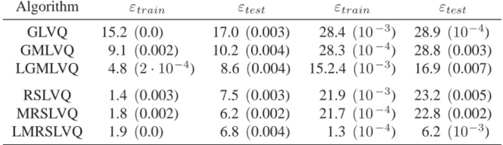
The obtained classification accuracies are summarized in Table 3. For both cost function schemes the performance improves with increasing complexity of the distance measure, except for Local MRSLVQ which shows overfitting effects. Remarkably, RSLVQ and MRSLVQ clearly outperform the respective GLVQ methods on this data set. Regarding GLVQ and RSLVQ, this observation is solely based on different

pro-totype constellations. The algorithms identify similarw for classes with low rate of

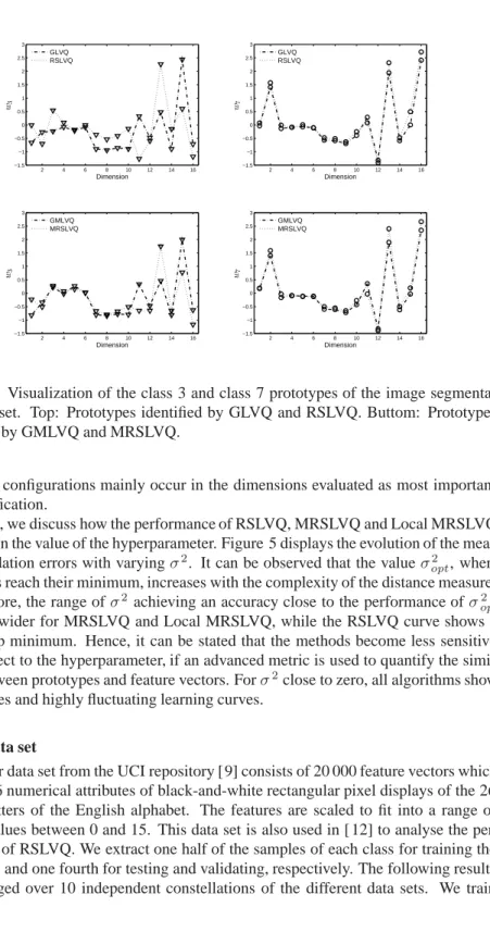
misclassification. Differences can be observed in case of prototypes, which contribute strongly to the overall test error. For demonstration purposes, we refer to classes 3 and

7. The mean class specific test errors constitute_ε3_test= 25.5%and_ε7_test= 1.2%for the

GLVQ classifiers and_ε3_test = 10.3and_ε7_test = 1.2%for the RSLVQ classifiers. The

respective prototypes obtained in one cross validation run are visualized in Figure 3. It depicts that the algorithms identify nearly the same representative for class 7, while the class 3 prototypes reflect differences for the alternative learning strategies. This finding holds similarly for the GMLVQ and MRSLVQ prototypes, however, it is less pronounced (see Figure 3).

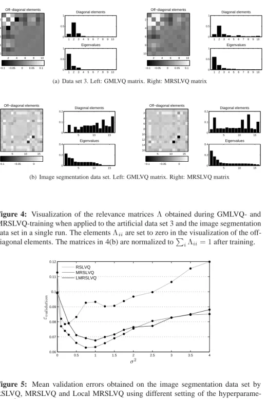
The varying classification performance of the two latter methods also goes back to different metric parameter settings derived during training. Comparing the relevance matrices (see Figure 4) shows that GMLVQ and MRSLVQ identify the same dimen-sions as being most discriminative to classify the data. The features which achieve the highest weight values on the diagonal are the same in both cases. But note, that the feature selection by MRSLVQ is more pronounced. Interestingly, differences in the

(17)

2 4 6 8 10 12 14 16 −1.5 −1 −0.5 0 0.5 1 1.5 2 2.5 3 Dimension w3 GLVQ RSLVQ 2 4 6 8 10 12 14 16 −1.5 −1 −0.5 0 0.5 1 1.5 2 2.5 3 Dimension w7 GLVQ RSLVQ 2 4 6 8 10 12 14 16 −1.5 −1 −0.5 0 0.5 1 1.5 2 2.5 3 Dimension w3 GMLVQ MRSLVQ 2 4 6 8 10 12 14 16 −1.5 −1 −0.5 0 0.5 1 1.5 2 2.5 3 Dimension w7 GMLVQ MRSLVQ

Figure 3: Visualization of the class 3 and class 7 prototypes of the image

segmenta-tion data set. Top: Prototypes identified by GLVQ and RSLVQ. Buttom: Prototypes identified by GMLVQ and MRSLVQ.

prototype configurations mainly occur in the dimensions evaluated as most important for classification.

Finally, we discuss how the performance of RSLVQ, MRSLVQ and Local MRSLVQ depends on the value of the hyperparameter. Figure 5 displays the evolution of the mean

final validation errors with varying_σ2. It can be observed that the value_σ2_opt, where

the curves reach their minimum, increases with the complexity of the distance measure.

Furthermore, the range of_σ2 achieving an accuracy close to the performance of_σ2_opt

becomes wider for MRSLVQ and Local MRSLVQ, while the RSLVQ curve shows a very sharp minimum. Hence, it can be stated that the methods become less sensitive with respect to the hyperparameter, if an advanced metric is used to quantify the

simi-larity between prototypes and feature vectors. For_σ2close to zero, all algorithms show

instabilities and highly fluctuating learning curves.

Letter data set

The Letter data set from the UCI repository [9] consists of 20 000 feature vectors which encode 16 numerical attributes of black-and-white rectangular pixel displays of the 26 capital letters of the English alphabet. The features are scaled to fit into a range of integer values between 0 and 15. This data set is also used in [ 12] to analyse the per-formance of RSLVQ. We extract one half of the samples of each class for training the classifiers and one fourth for testing and validating, respectively. The following results are averaged over 10 independent constellations of the different data sets. We train

(18)

Experiments Off−diagonal elements 2 4 6 8 10 2 4 6 8 10 −0.1 −0.05 0 0.05 0.1 1 2 3 4 5 6 7 8 910 0 0.5 1 Diagonal elements 1 2 3 4 5 6 7 8 910 0 0.5 1 Eigenvalues Off−diagonal elements 2 4 6 8 10 2 4 6 8 10 −0.1 −0.05 0 0.05 0.1 1 2 3 4 5 6 7 8 910 0 0.5 1 Diagonal elements 1 2 3 4 5 6 7 8 910 0 0.5 1 Eigenvalues

(a) Data set 3. Left: GMLVQ matrix. Right: MRSLVQ matrix

Off−diagonal elements 5 10 15 2 4 6 8 10 12 14 16 −0.1 −0.05 0 5 10 15 0 0.1 0.2 Diagonal elements 5 10 15 0 0.2 0.4 Eigenvalues Off−diagonal elements 5 10 15 2 4 6 8 10 12 14 16 −0.1 −0.05 0 5 10 15 0 0.1 0.2 Diagonal elements 5 10 15 0 0.2 0.4 Eigenvalues

(b) Image segmentation data set. Left: GMLVQ matrix. Right: MRSLVQ matrix

Figure 4: Visualization of the relevance matricesΛ obtained during GMLVQ- and MRSLVQ-training when applied to the artificial data set 3 and the image segmentation

data set in a single run. The elementsΛii are set to zero in the visualization of the

off-diagonal elements. The matrices in 4(b) are normalized to_iΛii= 1after training.

0 0.5 1 1.5 2 2.5 3 3.5 4 0.06 0.07 0.08 0.09 0.1 0.11 0.12 σ2 εva li da ti on RSLVQ MRSLVQ LMRSLVQ

Figure 5: Mean validation errors obtained on the image segmentation data set by

RSLVQ, MRSLVQ and Local MRSLVQ using different setting of the

(19)

the classifiers with one prototype per class respectively and use the learning parameter settings

(Local) G(M)LVQ:α1= 0.1,α2= 0.01,c= 0.1

(Local) (M)RSLVQ:α1= 0.01,α2= 0.001,c= 0.1.

Training is continued for 150 epochs in total with different values_σ2lying in the

inter-val [0.75, 4.0]. The accuracy on the inter-validation set is used to select the best settings for

the hyperparameter. With the settings_σ_opt2 (RSLVQ) = 1.0and_σ2_opt(MRSLVQ_,Local

MRSLVQ) = 1.5 we achieve the performances stated in Table 3. The results depict

that training of an individual metric for every prototype is particularly efficient in case of multi-class problems. The adaptation of a global relevance matrix does not provide significant benefit because of the huge variety of classes in this application. Simi-lar to the previous application, the RSLVQ-based algorithms outperform the methods based on the GLVQ cost function. Remarkably, the classification accuracy of Local MRSLVQ with one prototype per class is comparable to the RSLVQ results presented

in [12], achieved with constant hyperparameter_σ2 and 13 prototypes per class. This

observation underlines the crucial importance of an appropriate distance measure for the performance of LVQ-classifiers. Despite the large number of parameters, we do not observe overfitting effects during training of local relevance matrices on this data set. The systems show stable behaviour and converge within 100 training epochs.

5 Conclusions

We have considered metric learning by matrix adaptation in discriminative vector quan-tization schemes. In particular, we have introduced this principle into soft robust learn-ing vector quantization, which is based on an explicit statistical model by means of mix-tures of Gaussians, and we extensively compared this method to an alternative scheme derived from an intuitive but somewhat heuristic cost function. In general, it can be ob-served that matrix adaptation allows to improve the classification accuracy on the one hand, and it leads to a simplification of the classifier and thus better interpretability of the results by inspection of the eigenvectors and eigenvalues on the other hand. Inter-estingly, the behavior of GMLVQ and MRSLVQ shows several principled differences. Based on the experimental findings, the following conclusions can be drawn:

• All discriminative vector quantization schemes show good generalization

behav-ior and yield reasonable classification accuracy on several benchmark results us-ing only few prototypes. RSLVQ seems particularly suited for the real-life data sets considered in this article. In general, matrix learning allows to further im-prove the results, whereby, depending on the setting, overfitting can be more pronounced due to the huge number of free parameters.

• The methods are generally robust against noise in the data as can be inferred

(20)

Derivatives

GLVQ and variants are rather robust to the choice of hyperparameters, a very

critical hyperparameter of training is the softness parameter_σ2for RSLVQ.

Ma-trix adaptation seems to weaken the sensitivity w.r.t. this parameter, however, a

correct choice of_σ2is still crucial for the classification accuracy and efficiency

of the runs. For this reason, automatic adaptation schemes for_σ2should be

con-sidered. In [13], a simple annealing scheme for_σ2 is introduced which yields

reasonalbe results. We are currently working on a scheme which adapts_σ2in a

more principled way according to an optimization of the likelihood ratio showing first promising results.

• The methods allow for an inspection of the classifier by means of the

proto-types which are defined in input space. Note that one explicit goal of

unsuper-vised vector quantization schemes such as_k-means or the self-organizing map is to represent typical data regions be means of prototypes. Since the considered approaches are discriminative, it is not clear in how far this property is main-tained for GLVQ and RSLVQ variants. The experimental findings demonstrate that GLVQ schemes place prototypes close to class centres and prototypes can be interpreted as typical class representatives. On the contrary, RSLVQ schemes do not preserve this property in particular for non-overlapping classes since adap-tation basically takes place based on misclassifications of the data. Therefore, prototypes can be located outside the class centers while maintaining the same or a similar classification boundary compared to GLVQ schemes. This property has already been observed and proven in typical model situations using the theory of online learning for the limit learning rule of RSLVQ, learning from mistakes, in [2].

• Despite the fact that matrix learning introduces a huge number of additional free

parameters, the method tends to yield very simple solutions which involve only few relevant eigendirections. This behavior can be substantiated by an exact mathematical investigation of the LVQ2.1-type limit learning rules which result

for small_σ2 or a steep sigmoidal functionΦ, respectively. For these limits, an

exact mathematical investigation becomes possible, indicating that a unique so-lution for matrix learning exist, given fixed prototypes, and that the limit matrix reduces to a singular matrix which emphasizes one major eigenvalue direction. The exact mathematical treatment of these simplified limit rules is subject of on-going work and will be published in subsequent work.

In conclusion, systematic differences of GLVQ and RSLVQ schemes result from the different cost functions used in the approaches. This includes a larger sensitivity of RSLVQ to hyperparanmeters, a different location of prototypes which can be far from the class centres for RSLVQ, and different classification accuracies in some cases. Apart from these differences, matrix learning is clearly beneficial for both discrimi-native vector quantization schemes as demonstrated in the experiments.

(21)

A

Derivatives

We compute the derivatives of the RSLVQ cost function with respect to the proto-types, the metric parameters, and the hyperparameters. More generally, we compute

the derivative of the likelihood ratio with respect to any parameterΘ_i =ξ. The

con-ditional densities can be chosen to have the normalized exponential formp(ξ|j) =

K(j)·expf(ξ,wj, σj2,Ωj). Note that the normalization factorK(j)depends on the

shape of component_j. If a mixture of_N-dimensional Gaussian distributions is

as-sumed,_K(j) = (2πσj2)(−N/2) is only valid under the constraintdet(Λj) = 1. We

point out that the following derivatives subject to the conditiondet(Λ_j) =const.∀j.

Withdet(Λ_j) = const.∀j, the_K(j)as defined above are scaled by a constant

fac-tor which can be disregarded. The condition of equal determinant for all_j naturally

includes the adaptation of a global relevance matrixΛ = Λ_j,∀j.

(22)

Derivatives =δy,c(wi)(Py(i|ξ)−P(i|ξ)) 1 K(i) ∂K(i) ∂Θi + ∂f(ξ,wi, σ2i,Ωi) ∂Θi −(1−δy,c(wi))P(i|ξ) 1 K(i) ∂K(i) ∂Θ_i + ∂f(ξ,wi, σi2,Ωi) ∂Θ_i (25) with(a) ∂p(ξ, y|W) ∂Θi = ∂ ∂Θ_i j:c(wj)=y P(j)p(ξ|j) = j δy,c(wj)P(j) ∂p(ξ|j) ∂Θ_i = j δy,c(wj)P(j) expf(ξ,wj, σj2,Ωj) ∂K(j) ∂Θ_i +K(j) ∂f(ξ,wj, σj2,Ωj) ∂Θ_i and(b) c=y ∂p(ξ, c|W) ∂Θ_i = ∂ ∂Θ_i j:c(wj)=y P(j)p(ξ|j) = j (1−δy,c(wj))P(j) ∂p(ξ|j) ∂Θ_i = j (1−δy,c(wj))P(j) expf(ξ,wj, σj2,Ωj) ∂K(j) ∂Θi +K(j) ∂f(ξ,wj, σj2,Ωj) ∂Θi

(23)

Py(i|ξ)andP(i|ξ)are assignment probabilities, Py(i|ξ) = P(i)K(i) expf(ξ,wi, σ 2 i,Ωi) p(ξ, y|W) = P(i)K(i) expf(ξ,wi, σ 2 i,Ωi) j:c(wj)=yP(j)K(j) expf(ξ,wj, σ2j,Ωj) P(i|ξ) = P(i)K(i) expf(ξ,wi, σ 2 i,Ωi) p(ξ|W) = P(i)K(i) expf(ξ,wi, σ 2 i,Ωi) jP(j)K(j) expf(ξ,wj, σ2j,Ωj)

Py(i|ξ)constitutes the probability that sample ξis assigned to component i of the

correct classyandP(i|ξ)depicts the probability theξis assigned to any componenti

of the mixture.

The derivative with respect to a global parameter, e.g. a global matrixΩ = Ω_jfor all_j

can be derived thereof by summation.

References

[1] B. Arnonkijpanich, B. Hammer, A. Hasenfuss, and A. Lursinap. Matrix learning for topographic neural maps. In ICANN’2008, 2008.

[2] M. Biehl, A. Ghosh, and B. Hammer. Dynamics and generalization ability of LVQ algorithms. Journal of Machine Learning Research, 8:323–360, 2007.

[3] T. Bojer, B. Hammer, D. Schunk, and K. Tluk von Toschanowitz. Relevance determination in learning vector quantization. In M. Verleysen, editor, European

Symposium on Artificial Neural Networks, pages 271–276, 2001.

[4] K. Crammer, R. Gilad-Bachrach, A. Navot, and A. Tishby. Margin analysis of the lvq algorithm. In Advances in Neural Information Processing Systems, volume 15, pages 462–469. MIT Press, Cambridge, MA, 2003.

[5] B. Hammer, M. Strickert, and T. Villmann. On the generalization ability of GR-LVQ networks. Neural Processing Letters, 21(2):109–120, 2005.

[6] B. Hammer and T. Villmann. Generalized relevance learning vector quantization.

Neural Networks, 15(8-9):1059–1068, 2002.

[7] Samuel Kaski. Principle of learning metrics for exploratory data analysis. In

Neural Networks for Signal Processing XI, Proceedings of the 2001 IEEE Signal Processing Society Workshop, pages 53–62. IEEE, 2001.

(24)

References

[8] T. Kohonen. Self-Organizing Maps. Springer, Berlin, Heidelberg, second edition, 1997.

[9] D. J. Newman, S. Hettich, C. L. Blake, and C. J. Merz. Uci repository of machine

learning databases. http://archive.ics.uci.edu/ml/, 1998.

[10] A. Sato and K. Yamada. Generalized learning vector quantization. In M. C. Mozer D. S. Touretzky and M. E. Hasselmo, editors, Advances in Neural Information

Processing Systems 8. Proceedings of the 1995 Conference, pages 423–9,

Cam-bridge, MA, USA, 1996. MIT Press.

[11] P. Schneider, M. Biehl, and B. Hammer. Adaptive relevance matrices in learning vector quantization. Submitted, 2007.

[12] Sambu Seo and Klaus Obermayer. Soft learning vector quantization. Neural

Computation, 15(7):1589–1604, 2003.

[13] Sambu Seo and Klaus Obermayer. Dynamic hyper parameter scaling method for lvq algorithms. In International Joint Conference on Neural Networks, Vancouver, Canada, 2006.

[14] M. Strickert, K. Witzel, H.-P. Mock, F.-M. Schleif, and T. Villmann. Supervised attribute relevance determination for protein identification in stress experiments. In Proceedings of Machine Learning in Systems Biology, 2007.

[15] Kilian Weinberger, John Blitzer, and Lawrence Saul. Distance metric learning for large margin nearest neighbor classification. In Y. Weiss, B. Schölkopf, and J. Platt, editors, Advances in Neural Information Processing Systems 18, pages 1473–1480. MIT Press, Cambridge, MA, 2006.

(25)

Table 2: Mean rate of misclassification (in %) obtained by the different algorithms on

the artificial data sets 3 and 4 at the end of training. The values in brackets constitute the variances.

Data set 3 Data set 4

GLVQ 23.5 (0.1) 38.0 (0.2) 31.2 (0.06) 41.0 (0.2)

GMLVQ 12.1 (0.1) 24.0 (0.36) 14.5 (0.1) 30.6 (0.5)

RSLVQ 4.1 (0.1) 33.2 (0.5) 11.7 (0.1) 36.8 (0.17)

MRSLVQ 3.9 (0.08) 29.5 (0.4) 8.0 (0.08) 32.0 (0.22)

Table 3: Mean rate of misclassification (in %) obtained by the different algorithms on

the image segmentation and letter data set at the end of training. The values in brackets constitute the variances.

Image segmentation data Letter data

GLVQ 15.2 (0.0) 17.0 (0.003) 28.4 (10−3) 28.9 (10−4) GMLVQ 9.1 (0.002) 10.2 (0.004) 28.3 (10−4) 28.8 (0.003) LGMLVQ 4.8 (2·10−4) 8.6 (0.004) 15.2.4 (10−3) 16.9 (0.007) RSLVQ 1.4 (0.003) 7.5 (0.003) 21.9 (10−3) 23.2 (0.005) MRSLVQ 1.8 (0.002) 6.2 (0.002) 21.7 (10−4) 22.8 (0.002) LMRSLVQ 1.9 (0.0) 6.8 (0.004) 1.3 (10−4) 6.2 (10−3)