Extreme Point-based Heuristics for Three-Dimensional Bin
Packing
Teodor Gabriel Crainic
D´epartement de management et technologie Ecole des sciences de la gestion, U.Q.A.M.
and CIRRELT, Montreal (Canada) e-mail: [email protected]
Guido Perboli ∗
Department of Control and Computer Engineering Politecnico di Torino
Corso Duca degli Abruzzi, 24 - I-10129, Torino (Italy) Tel: +39 011 5647097
Fax: +39 011 5647099 e-mail: [email protected]
Roberto Tadei
Department of Control and Computer Engineering Politecnico di Torino, Torino (Italy)
e-mail: [email protected]
Abstract
One of the main issues in addressing three-dimensional packing problems is finding an efficient and accurate definition of the points where to place the items inside the bins, as the performance of exact and heuristic solution methods is actually strongly influenced by the choice of a placement rule. We introduce the Extreme Point concept and present a new Extreme Point-based rule for packing items in-side a three-dimensional container. The Extreme Point rule is independent from the particular packing problem addressed and can handle additional constraints, such as fixing the position of the items. The new Extreme Point rule is also used to derive new constructive heuristics for the Three-Dimensional Bin Packing problem. Extensive computational results show the effectiveness of the new heuristics com-pared to state-of-the-art results. Moreover, the same heuristics, when applied to the Two-Dimensional Bin Packing problem, outperform those specifically designed for the problem.
Keywords: Programming, Integer, Algorithms, Heuristic; Three-dimensional pack-ing; bin packing.
1.
Introduction
One of the main issues in addressing multi-dimensional packing problems is the definition of the position where to place the items inside the container (Lodi et al. 2002a, 1999b; Perboli 2002) . The performance in terms of computational efficiency and solution qual-ity of exact and heuristic solution methods for multi-dimensional packing problems is actually very sensitive to the item-positioning rule (Lodi et al. 2004) . While the issue is not relevant for mono-dimensional packing problems, it is harder to address in the three-dimensional case than in the two-dimensional one. Thus, the approaches used for two-dimensional problems cannot generally be extended to the three-dimensional case or, in the best case, the extension yields a packing where the volume of the bins is underutilized (Lodi et al. 2002a,b) .
We introduce a new rule for packing items inside a container, the Extreme Point (EP)
rule, which is independent from the particular packing problem addressed. The EP rule
can be applied to any 3D and 2D packing problem, as well as to packing problems with additional constraints, e.g., when the accommodation of the items must follow
fixed positions inside the container. The new EP rule is also efficient relative to both
the computational effort and the resulting container-volume utilization. On the one
hand, the EPs of a given packing are polynomially computable. On the other hand,
when applied within packing heuristics, the EP rule allows to significantly improve the
utilization of the container volumes and, thus, the performance of the respective method.
We derive new EP-based heuristics to efficiently address the Three-Dimensional
(3D-BP) and the Two-Dimensional (2D-BP) Bin Packing problems. Given a set of
rectangular-shaped items i ∈ I with sizes wi, di, and hi, and an unlimited number of
containers of fixed sizes W, D, and H, called bins, the 3D-BP problem consists in
or-thogonally packing, without overlapping, all the items into the minimum number of bins.
We assume that the items cannot be rotated. In the 2D-BP problem, the heightshi and
H of items and bins, respectively, are ignored.
TheEP idea is used to design modified versions of the well-known First Fit
Extensive computational results show that the newEP-based constructive heuristics ap-plied to benchmark test instances yield results that improve over those obtained by the
existing constructive heuristics. Moreover, we derive an EP-based composite heuristics
that, with a negligible computational effort, outperforms existing constructive heuristics
for both the3D-BP and2D-BP problems, as well as state-of-the-art meta-heuristics and
Branch & Bound methods.
The paper is organized as follows. Section 2 summarizes the methods previously
pro-posed to place items into containers and solve the 3D-BP problem. Extreme Points are
introduced in Section 3, while Section 4 is dedicated to presenting the new constructive heuristics. Computational results are presented and discussed in Section 5.
2.
Literature Review
We review the literature along two directions: first, the methods proposed to place items into a container; second, solution methods for the three-dimensional bin packing problem.
2.1 Placement of items into two and three-dimension containers
A first attempt to model multi-dimensional packings is due to Gilmore and Gomory (Gilmore and Gomory 1965) . They proposed a representation given by the enumeration of all thepatterns, i.e., the subsets of items that could be accommodated into a container, given the problem constraints. The huge number of patterns that can be defined from a given set of items makes the approach appropriate for column-generation approaches only (Gilmore and Gomory 1965; Baldacci and Boschetti 2007) .
Beasley (Beasley 1985) considered a formulation for 2D packings based on the
dis-cretization of the container’s surface into p×q rectangles. The bottom-left corner of
each item was then placed on the bottom-left corner of a rectangle. A similar represen-tation was introduced by Hadjiconstantinou and Christofides (Hadjiconstantinou and Christofides 1995) , except that instead of explicitly partitioning the container into
rect-angles, they limited the set of coordinates each item could assume to p and q values.
In both cases, the number of variables grows with the accuracy of the discretization. Therefore, such representation are principally used to compute upper bounds through Lagrangian relaxation and subgradient optimization.
shelves_example.png
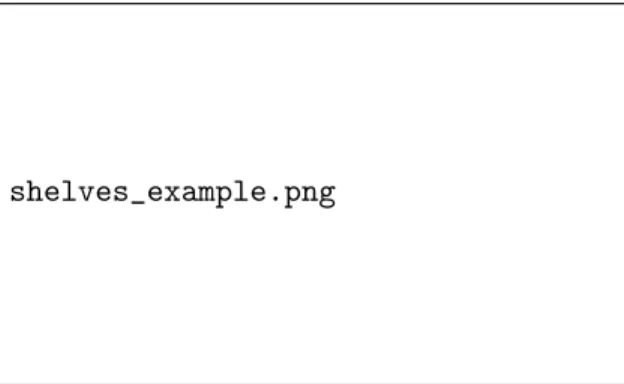
An approach often used for 2D-packing building consists in combining procedures
designed for mono-dimensional problems and so-calledshelf (orlayer) methods (Chung
et al. 1982; Berkey and Wang 1987) . The items are first sorted and packed into “shelves” with sizes equal to the width of the box. The problem then reduces to solving a mono-dimensional packing instance. Indeed, a 2D packing can be obtained by placing the shelves into the containers according to the solution of a mono-dimensional packing problem, where the size of the items equals the depth of the shelves and the size of the
mono-dimensional containers equals the depthDof the two-dimensional ones. The same
approach can also be used to build 3D packings. Build first two-dimensional shelves by using any 2D algorithm and, then, arrange them into the three-dimensional containers by solving a mono-dimensional packing problem, where the size of the items equals
the height of the shelves and the size of the containers equals the height H. When
the 2D shelves are also built according to the shelf approach, the method is known as
wall-building (George and Robinson 1980; Pisinger 2002) . The drawback of the shelf approach is that it introduces guillotine cuts on the depth and height of the two and three-dimensional bins, respectively, leading to the underutilization of the containers. Figure 1 illustrates 2D and 3D packings obtained by means of the shelf approach.
fig_corner_points.png
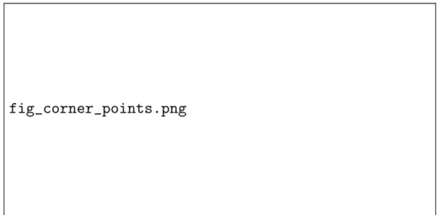
Figure 2: Corner Points in 3D and 2D Packings
Martello, Pisinger, and Vigo (Martello et al. 2000) defined Corner Points as the
non-dominated locations where an item can be placed into an existing packing. In two dimensions, Corner Points are defined where the envelope of the items in the bin changes from vertical to horizontal (the large black dots in Figure 2b). Corner Points on the three-dimensional envelope can be found applying the two-dimensional algorithm for each distinct value of the height of the bin defined by the lower and upper terminal lines of each item (see Figure 2a for an example of Corner Points in three dimensions). A
Corner Point set can be computed in O(n2). Martello, Pisinger, and Vigo (Martello
et al. 2000) used this idea to design a Branch & Bound algorithm to verify whether a
given set of items can be packed into a container or not. den Boefet al. (den Boef et al.
2005) showed that the algorithm to compute the Corner Points presented in (Martello
et al. 2000) may miss some feasible packings. Martello et al. (Martello et al. 2007)
addressed this issue by providing a new version of the procedure to compute the Corner Points, as well as an updated version of the related Branch & Bound algorithm.
The utilization of Corner Points in Branch & Bound algorithms drastically reduces the number of partial solutions explored. Constructive heuristics using Corner Points can be inefficient in terms of container utilization, however, because the definition of Corner Points depends on the sequence of the accommodation of the items into the container. Consider, for example, the packing depicted in Figure 2b and item 11. According to the definition of the Corner Points, one can add the item on any of the large black dots. It is clear, however, that item 11 could also be placed into one of the shaded regions, which the Corner Points do not allow to exploit. The space lost in three dimensional packings could be significant, particularly when the sizes of the items vary a lot. Consider, for example, Figure 2a where the placement of the large item on top of the packing causes a large volume below it to become unavailable for future items.
iggraph_example.png
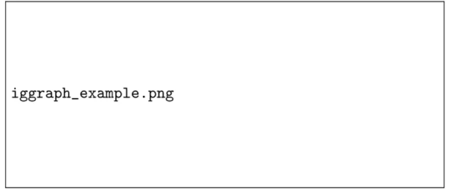
Figure 3: Packings and Associated Interval Graphs According to Fekete and Schepers A graph-theoretical approach for the characterization of multi-dimensional packings has been proposed by Fekete and Schepers (Fekete and Schepers 1997, 2001) . The authors considered the relative positions of the items in a feasible packing and defined a graph describing the item “overlapping” according to the projection of the items on
each orthogonal axis. More formally, let Gd(V, Ed) be the interval graph associated to
the dth axis. Each vertex of Gd(V, Ed) is associated to an item iin the container and a
non-oriented edge (i, j) between two itemsiand j exists if and only if their projections
on axisdoverlap (see Figure 3). The authors proved necessary conditions on the interval
graphs to define a feasible packing. Combined to good heuristics for dismissing infeasible subsets of items, this characterization was used to develop a two-level tree search (Fekete and Schepers 1997) . According to computational results, mainly limited to 2D problems, this strategy outperforms previous methods. Unfortunately, however, the method cannot handle additional constraints on the packing, such as fixing the position of one or more
items. No direct comparison with the Branch & Bound of Martello et al. (Martello
et al. 2007) has been performed yet. The link between guillotine cuts and interval graphs has been analyzed by Perboli (Perboli 2002) .
2.2 Solution methods for the 3D-BP problem
The first exact method for the 3D-BP problem, a two level Branch & Bound, was
pro-posed by Martello, Pisinger, and Vigo (Martello et al. 2000) . The first search level assigned items to bins. At each node of the first-level tree, a second level Branch &
Bound was used to verify whether the items assigned to each bin can be packed into it using current Corner Points (Subsection 2.1). The authors tested their procedure on 6
sets of instances with up to 90 items. Martello et al. (Martello et al. 2007) improved
this Branch & Bound by fixing the procedure that verifies the Corner Points.
The first lower bounds for the 3D-BP problem have been presented by Martello,
Pisinger, and Vigo (Martello et al. 2000) . Their best bound considered the items with
width and height larger than p andq, respectively, and determined the subsets of items
that, for geometric reasons, can not be placed side by side. A new class of lower bounds has been introduced by Fekete and Schepers (Fekete and Schepers 1997) . The authors extended the use of dual-feasible functions, initially introduced by Johnson (Johnson
1973) , to two and three dimensional packing problems, including the 3D-BP problem.
The most recent lower bound, due to Boschetti (Boschetti 2004) , introduces new dual feasible functions. The bound dominates the bounds by Martello, Pisinger, and Vigo and by Fekete and Schephers.
A Tabu Search algorithm for the 2D-BP problem was proposed by Lodi, Martello,
and Vigo (Lodi et al. 1999a) . The algorithm consisted of two simple constructive
heuristics to pack the items into bins, and a Tabu Search mechanisms to control the movement of items between bins. Two neighborhoods were considered to try to move an item from the weakest bin (i.e., the bin that appeared to be the easiest to empty) into another. Since the constructive heuristics produced guillotine packings, so did the
overall algorithm. The authors generalized this approach to other variants of the BP
problem, including the one considered in this paper (Lodi et al. 2004) .
Faroe, Pisinger, and Zachariasen presented a Guided Local Search (GLS) heuristic for the3D-BP problem (Faroe et al. 2003) . Starting with an upper bound on the number of bins obtained by a greedy heuristic procedure, the algorithm iteratively decreased the number of bins, each time searching for a feasible packing using the GLS method. The process terminated when either a given time limit was reached or the current solution matched a precomputed lower bound. Computational experiments were reported for 2 and 3-dimension instances with up to 200 items.
Two constructive heuristics have been developed and tested for the3D-BP problem
by Martello, Pisinger, and Vigo (Martello et al. 2000) . The first algorithm, called
S-Pack, was based on a layer-building principle derived from the shelf approaches described
in Subsection 2.1. The second heuristic, denotedMPV-BS, repeatedly filled one bin after
the other by means of the Branch & Bound algorithm for the single container presented by the authors in the same paper. To reduce the computational time of the algorithm, the Branch & Bound is truncated by limiting the width of the tree.
Lodi, Martello, and Vigo presented a new shelf-based heuristic for the3D-BP, called
Height first - Area second (HA) (Lodi et al. 2002b) . The algorithm was based on constructing two solutions and selecting the best. To obtain the first one, items were partitioned into clusters according to their height and a series of layers were obtained from each cluster. The layers were then packed into bins using the Branch & Bound
algorithm by Martello and Toth for the 1D-BP problem (Martello and Toth 1990) .
The second solution was obtained by ordering the items by non-increasing area of their base and building new layers. As previously, layers were packed into bins by solving a
1D-BP problem. HA is the constructive heuristic that currently obtains the best results on the benchmark test problem instances.
Notice that none of the reviewed constructive heuristics has a polynomial
computa-tional effort. They actually use a Branch & Bound algorithm to pack the shelves (S-Pack
and HA) or build the accommodation (S-Pack).
3.
Extreme Points: An Efficient Rule for the Placement of
Items in Three Dimensions
The main contribution of this paper is the introduction of a new accurate and efficient procedure to place items inside a container. The procedure is based on the concept of
Extreme Points (EPs). The Extreme Points idea extends the Corner Points concept.
EPs provide the means to exploit the free space defined inside a packing by the shapes
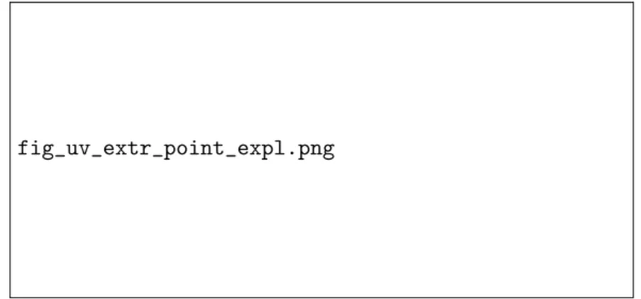
of the items already in the container. Figure 4 illustrates EPs in 3D and 2D packings.
fig_uv_extr_point_expl.png
Figure 4: Example of Definition of Extreme Points in 3D and 2D Packings
The basic idea of theEPs is that when an item kwith sizeswk,dk, andhk is added
to a given packing and is placed with its left-back-down corner in position (xk, yk, zk),
it generates a series of new potential points, the EPs, where additional items can be
accommodated. The new EPs are generated by projecting the points with coordinates
(xk+wk, yk, zk), (xk, yk+dk, zk), and (xk, yk, zk +hk) on the orthogonal axes of the container. Figure 5 illustrates the concept.
Given a packing and the list3DEPLof Extreme Points defined by the items already
in the packing, Algorithm 1 finds the new EPs that must be added to the list following
the placement of item k in position (xk, yk, zk). The main idea of Algorithm 1 is as
follows (to facilitate the reading of the paper, the pseudo-codes of all algorithms are presented in Appendix I):
• If the container is empty, the item is placed in position (0, 0, 0), which generates
three EPs in positions (wk, 0, 0), (0,dk, 0), and (0, 0,hk);
• Otherwise, the item is placed in position (xk,yk,zk) and newEPs are obtained by projecting
fig-ep-singleitem.png
Figure 5: EPs defined by an item (the EP are the triangles)
– Point (xk+wk, yk, zk) in the directions of the Y andZ axes,
– Point (xk, yk+dk, zk) in the directions of the X and Z axes, and
– Point (xk, yk, zk+hk) in the directions of the X and Y axes.
Each point is projected on all items lying between item k and the wall of the
container in the respective direction;
• If there are more than one item on which a point can be projected, the algorithm
chooses the nearest one.
Algorithm 1 updates theEPs list, called 3DEP L, every time an item is added and
assumes knowledge of the EPs previously generated by the existing packing. It can
therefore be used within constructive heuristics, where items are added to each container one after the other. The computational complexity of the updating procedure is given by Theorem 1.
Theorem 1 Given a 3D-BPproblem instance and its set of items I, a sub-set of items
Ij ⊆ I already accommodated into a container j, the corresponding list 3DEPL of Ex-treme Points ordered by non increasing values of their positions onz, y, and xaxes, and an itemkthat can be accommodated into the container (i.e., for which one knows already the point where it can be placed without overlapping any other item in the container), the time complexity of Algorithm 1 is O(|Ij|).
Proof. Given item k, the Algorithm 1 generates six new EPs. For each item in Ij, one may verify in constant time whether the position of the new Extreme Points must
be updated. Thus, this verification phase is O(|Ij|). The new EPs are added to the
list 3DEPL. Because the list3DEPL is ordered, the insertion of the 6 newEPs requires 6 ∗ln(|Ij|) operations and the time complexity of the overall process is O(|Ij|+ 6∗
Notice that, because|Ij|is at most equal to n, where n=|I| is the total number of
items in the instance, the overall computational effort of Algorithm 1 is O(n).
4.
New
EP
-based Constructive Heuristics for the
3D-BP
Problem
The First Fit Decreasing (FFD) and the Best Fit Decreasing (BFD) procedures are
constructive heuristics for the 1D-BP problem. After an initial sorting of the items by
non-increasing order of their volumes, the two heuristics differ in how items are loaded. FFD heuristics load the ordered items one after the other in the first bin where they fit. BFD heuristics try to load each item in the best bin, i.e., the bin which, after loading the item, has the maximum free volume, defined as the bin volume minus the sum of the volumes of the items it contains. Both heuristics create a new bin when the item cannot be accommodated in the existing bins. Despite their simplicity, the FFD and
BFD heuristics offer good performances for the 1D-BP problem and adapting them to
the3D-BP problem appears an interesting perspective (Martello and Toth 1990) .
Unfortunately, extending the FFD and BFD heuristics to the 3D-BP problem is far
from trivial. On the one hand, while for the1D-BP case the ordering is done considering
the unique attribute characterizing both items and bins, i.e., their volume, more choices
exist in the 3D-BP context. One may thus consider sorting items according to their
width, height, or depth, as well as, derived from these attributes, according to their volume or the areas of their different faces. Consequently, the definition of the best bin
in the BFD heuristic is not unique for the 3D-BP problem. On the other hand, while
the item accommodation does not need to be considered in the 1D-BP problem, a 3D
packing may vary significantly according to how items are placed inside the bin, even when the ordering of the items and the best-bin selecting rules are not changed.
In the following, we propose new constructive heuristics, denoted FFD and EP-BFD, which extend the FFD and BFD heuristics, respectively, and place items into bins by using the Extreme Points. Both heuristics require the initial ordering of the items and sorting rules are described in Subsection 4.1. The EP-FFD and EP-BFD heuristics are then presented in Subsections 4.2 and 4.3, respectively.
4.1 Sorting the items
Different versions of the EP-FFD and EP-BFD heuristics can be defined by changing the ordering of the items. We tested several ordering rules. In the following, we present only those that experimentally yielded the best results.
• Volume-Height: Items are sorted by non-increasing values of their volume (wi×
di×hi). Items with the same volume are sorted by non-increasing values of their
height hi.
• Height-Volume: Items are sorted by non-increasing values of their heighthi. Items
with the same height are sorted by non-increasing values of their volume (wi×di×
• Area-Height: Items are sorted by non-increasing values of their base area (wi×di).
Items with the same area are sorted by non-increasing values of their height hi.
• Clustered Area-Height: Since two items have rarely the same base area, the second sorting criterion (“Height”) of the previous rule is not often used. In order to build
more regular packings, in the clustered version of the Area-Height ordering rule,
the bin area W ×Dis separated into clusters defined by the intervals:
Aj,δ = (j−1)×W D 100 δ, j×W D 100 δ .
where, W and D are the width and the depth of the bin, respectively, and δ ∈
[1,100]. Items are then assigned to clusters according to their base area and clusters
are ordered by decreasing values ofj. Items assigned to the same cluster are sorted
by non-increasing values of their heighthi.
• Height-Area: Items are sorted by non-increasing values of their height. Items
having the same height are sorted by non-increasing values of their base area (wi×
di).
• Clustered Height-Area: This rule is a variant of the previous one where, given a
valueδ ∈[1,100], the height H of the bin is separated into clusters defined by the
intervals: hj,δ = (j−1)×H 100 δ, j×H 100 δ .
Items are then assigned to clusters according to their height and clusters are ordered
by decreasing values of j. Items assigned to the same cluster are sorted by
non-increasing values of their base area (wi×di).
4.2 Extreme Point First Fit Decreasing heuristics
The Extreme Points First Fit Decreasing (EP-FFD) heuristic sorts the items according to a rule that can be externally specified. First, the algorithm verifies whether the item dimension is compatible with the bin size and discards it if it is not. A compatible item is loaded into the first existing bin where it fits; A new bin is created if the item cannot be loaded into any of the existing bins. To verify whether an item can be accommodated
into a bin, the EP-FFD heuristics places it on theEPs of the existing packing. An item
can be accommodated on an EP if, after placing its left-back-down corner on it, it does
not overlap any other item previously accommodated into the bin. If an item can be
placed on more than one EP inside the bin, the one with the lowest z, y,x coordinates
(in this order) is chosen. Every time an item is added, the EP-FFD heuristic is used to
update the list of the EPs.
Theorem 2 Given a 3D-BP problem instance I with n items, Algorithm EP-FFD has a time complexity of O(n3).
Proof. The EP-FFD heuristic tries to put each item into one of the existing bins. It
given EP. Recall that each item previously accommodated into a bin generates at most
6 EPs (Algorithm 1). Consequently, assuming there are m < n items already placed
into the bins, adding a new item kto the current solution requires the evaluation of at
most 6m EPs. The evaluation consists in cycling on the items already into the bin and
verifying whether item k overlaps any of them. This task can be accomplished in |Ib|,
where Ib is the set of items previously accommodated in the bin b. It is clear that the
worst case occurs when the algorithm has to check all themitems and thus, in the worst
case, 6m2 steps are required. When the item k cannot be placed in one of the existing
bins, a new bin is created and the item is accommodated into it in constant time.
Letbbe the bin where itemkhas been accommodated. According to Theorem 1, to
update theEP list ofbrequiresmsteps in the worst case (i.e., when all themitems have
been accommodated into the same bin). Thus, at mostO(6m2+m) steps are required to
accommodate a new itemk. Since the process is repeated for each item inI, Algorithm
EP-FFD takes O(n3).
4.3 Extreme Point Best Fit Decreasing heuristics
The Extreme Point Best Fit Decreasing (EP-BFD) heuristic sorts the items according to a rule that can be externally specified. First, the algorithm verifies whether the item dimension is compatible with the bin size and discards it if it is not. A compatible item
is loaded on the EP of the existing bin that maximizes a merit function measuring the
best bin and the best position where the item can be accommodated. Recall that, an item
can be accommodated on an EP if, after placing its left-back-down corner on it, it does
not overlap any other item previously accommodated into the bin. For each EP where
the item can be accommodated, a merit function is computed. If an item can be placed
on more than one EP, the one with the best merit function value is chosen. If the item cannot be loaded into any of the existing bins, a new bin is created. Every time an item
is added, Algorithm 1 is used to update the list of the EPs of the bin.
Consider a binb and an itemk, of dimensions wk,dk, and hk, to be loaded into the bin b. Let erepresent an EP inb with coordinates (xe, ye, ze). We tested several merit functions fb:
• Minimize the free volume after accommodating the item (FV). This is the
merit-function definition that is most similar to the one used in the1D-BP case. We place
the item into the bin which, once the item is in, displays the minimum amount of volume left. The merit function is defined as follows:
fb =Vb−
X
i∈b
vi−vk,
where Vb is the volume of the bin b and vi is the item volume. The main
disad-vantage of this merit function is that it does not use the information given by the
accommodation of the items inside the bin. Moreover, each EP in the bin has the
same merit value.
• Minimize the maximum packing size on the X and Y axes (MP). Each item is
axes of the resulting accommodation. Formally, the merit function is defined as follows: – The X axis fb = (xe+wk−WM P) ifxe+wk > WM P 0 otherwise – The Y axis fb = (ye+dk−DM P) ifye+dk> DM P 0 otherwise,
where WM P and DM P are the dimensions of the minimum box envelope of the
items accommodated beforek in the bin.
• Level the packing on X and Y axes (LEV). This rule is a modified version of the
previous one. It aims to level the packing on the X and Y axes, i.e., if the item
added increases the packing size, theEP yielding the minimum increase is chosen.
Otherwise, we consider theEP that minimizes the distance between the side of the
minimum box envelope of the packing and the side of the accommodated item. In this case the merit function that determines the best place for the accommodation is: – The X axis fb = (xe+wk−WM P)C ifx+wk> WM P (WM P −(xe+wk)) otherwise – The Y axis fb = (ye+dk−DM P)C ifye+dk > WM P (DM P −(ye+dk)) otherwise,
where C >max{W, D} is a high penalty on the increase of the dimensionsWM P
and DM P due to the new item.
• Maximize the utilization of the EPs’ Residual Space. The Residual Space (RS)
measures the free space available around an EP. Roughly speaking, the RS of an
EP is the distance, along each axis, from the bin edge or the nearest item. The
nearest item can be different on each axis. More precisely, when anEP is created,
its Residual Space on each axis is set equal to the distance from its position to the side of the bin along that axis (See Figure 6a). Every time an item is added to
the packing, the RS of all EPs are updated by means of Algorithm 2. Figure 6b
illustrates the concept. For “complex” packings, theRS gives only an estimate of
the effective volume available around the EPs and, thus, potential overlaps with
other items have to be verified when accommodating a new item on the chosenEP.
The merit function puts an item on theEP that minimizes the difference between
its RS and the item dimension:
fig_BFD_RSpace.png
Figure 6: Example ofResidual Space Definition
where RSex,RSye, and RSez are theRSs on X,Y, and Z axes, respectively.
When item k is added to the packing, the RSs are updated (see Algorithm 2 in
Appendix I) in O(n).
Theorem 3 Given an instance I of the 3D-BP problem with n items, the EP-BFD heuristic has a time complexity of O(n3+n∗max{n, O(U M F)}), whereO(U M F) is the complexity of the function which updates the merit function relative to a bin.
Proof. The EP-BFD heuristic tries to place each item into an existing bin. It verifies, for
eachEP of each bin, whether the item can be accommodated on it. Each item previously
accommodated in the bin generates at most 6 EPs (Algorithm 1). Consequently, adding
the item kto the bin b that already contains|Ib| items requires the verification of 6|Ib|
EPs. The verification consists in cycling on the items previously accommodated into the
bin to which the EP belongs and testing whether the itemk overlaps any other item in
the packing. This task can be accomplished in |Ib| time. If m < n items are already
in the bin, one must verify at most all the m items, requiring 6m2 steps to try to place
item kon all the existing EPs. When the item cannot be placed into the existing bins,
a new bin is allocated and the item is accommodated into it in constant time.
Let b be the bin where item k has been accommodated. The list of the EPs of b
is then updated in O(m) (Theorem 1), while updating the merit function of the items
loaded inbrequiresO(U M F) time. At mostO(6m2+ max{m, O(U M F)}steps are thus
required to accommodate the item k and, since the process is repeated for each item in
I, Algorithm EP-BFD takesO(n3+n∗max{n, O(U M F)}).
Lemma 4 Given an instance of the 3D-BP problem, Algorithm EP-BFD has a time complexity of O(n3) when it embeds one of the merit functions presented in Subsection 4.3.
All the merit functions can be updated in constant time, with the exception of the one
based on Residual Space, which requires O(n) (the Residual Space of each EP must
be updated - Algorithm 2). Thus, the time complexity of the U M F procedure is O(n)
for the merit functions presented in Section 4.3 and Algorithm EP-BFD is O(n3) by
Theorem 3.
5.
Computational Results
In this section, we analyze the computational results according to two different
view-points. Subsection 5.2 is dedicated to the analysis of the EP concept through a
compar-ison of the constructive heuristics using the CPs and the EPs, respectively. Secondly,
the results of the EP-FFD and EP-BFD heuristics are discussed. We start by compar-ing different versions of the EP-FFD and EP-BFD heuristics obtained by changcompar-ing the sorting rules (Subsections 5.3 and 5.4). A composite heuristic using the most effective sorting rules, denoted the C-EPBFD heuristic, is proposed in Subsection 5.5. The perfor-mance of the C-EPBFD heuristic is compared in Subsection 5.6 to that of all the existing constructive heuristics, as well as to that of more complex methods such as Branch &
Bound and meta-heuristic algorithms for the3D-BP problem. Moreover, the C-EPBFD
heuristic is also applied to the 2Dversion of theBP problem, its results being compared
to those of the best algorithms explicitly designed for the 2D-BP problem.
5.1 Test problems
Experiments were carried on standard benchmark instances for the 2D and 3D cases.
5.1.1 3D instances
The instances used for the 3D-BP problem came from Martello, Pisinger, and Vigo
(Martello et al. 2000) . For Classes I to V, the bin size is W =H =D= 100 and the
following five types of items are considered:
• Type 1: wj uniformly random in [1,12W], hj uniformly random in [23H, H], dj uniformly random in [23D, D];
• Type 2: wj uniformly random in [23W, W], hj uniformly random in [1,12H], dj uniformly random in [23D, D];
• Type 3: wj uniformly random in [23W, W], hj uniformly random in [23H, H], dj uniformly random in [1,12D];
• Type 4: wj uniformly random in [12W, W], hj uniformly random in [12H, H], dj uniformly random in [12D, D];
• Type 5: wj uniformly random in [1,12W], hj uniformly random in [1,12H], dj uniformly random in [1,12D].
For each of the first five classes, the items are:
• Class II: type 2 with probability 60%, type 1, 3, 4, 5 with probability 10% each;
• Class III: type 3 with probability 60%, type 1, 2, 4, 5 with probability 10% each;
• Class IV: type 4 with probability 60%, type 1, 2, 3, 5 with probability 10% each;
• Class V: type 5 with probability 60%, type 1, 2, 3, 4 with probability 10% each.
Classes fromVI toVIII were generated as follows:
• Class VI:wj,hj and dj uniformly random in [1,10] andW =H=D= 10;
• Class VII:wj,hj and dj uniformly random in [1,35] andW =H=D= 40;
• Class VIII:wj,hj and dj uniformly random in [1,100] and W =H =D= 100. For each class (i.e., I, IV, V, VI, VII, and VIII), we considered instances with a number of items equal to 50, 100, 150, and 200. Given a class and an instance size, we generated 10 different problem instances based on different random seeds. Bins are cubic in all instances. Following the experimental protocol of (Martello et al. 2000) , (Faroe et al. 2003) and (Crainic et al. forthcoming) , we did not consider the classes II and III because these have properties similar to those of class I.
5.1.2 2D instances
For the2D-BP problem, we considered ten classes of problems from (Berkey and Wang
1987) and (Martello and Vigo 1998) (the code of the generator and the instances are
available at http://www.or.deis.unibo.it/research.html). The first six classes have been
proposed by Berkey and Wang (Berkey and Wang 1987) :
• Class I:wj and hj uniformly random in [1,10] andW =H = 10;
• Class II:wj andhj uniformly random in [1,10] andW =H= 30;
• Class III:wj and hj uniformly random in [1,35] andW =H= 40;
• Class IV:wj and hj uniformly random in [1,35] andW =H= 100;
• Class V:wj andhj uniformly random in [1,100] andW =H= 100;
• Class VI:wj and hj uniformly random in [1,100] andW =H= 300.
In each class, all the item sizes were generated within the same interval. Martello and Vigo (Martello and Vigo 1998) have proposed more realistic test cases where items are classified into four types:
• Type 1: wj uniformly random in [23W, W],hj uniformly random in [1,12H];
• Type 2: wj uniformly random in [1,12W], hj uniformly random in [23H, H];
• Type 3: wj uniformly random in [12W, W],hj uniformly random in [12H, H];
The bin sizes are W = H = 100 for all test classes, while the items are defined according to the following rules:
• Class VII: type 1 with probability 70%, type 2, 3, 4 with probability 10% each;
• Class VIII: type 2 with probability 70%, type 1, 3, 4 with probability 10% each;
• Class IX: type 3 with probability 70%, type 1, 2, 4 with probability 10% each;
• Class X: type 4 with probability 70%, type 1, 2, 3 with probability 10% each. For each class, we considered instances with a number of items equal to 20, 40, 60, 80, and 100. For each class and item size, 10 instances were generated.
We directly applied our heuristics for the3D-BP problem to these 2D instances by
adapting them as follows:
• TheX andY dimensions of the three-dimensional instances were set to theX and
Y sizes of the two-dimensional ones, respectively;
• The Z dimensions of the items of the three-dimensional instances were set equal
to theZ size of the three-dimensional bin.
5.2 An Extreme versus Corner Points comparison
In order to compare the CP and EP concepts, we developed a version of the FFD
heuristics where the CPs are used for the placement of the items instead of the EPs.
We tested the CP-FFD and EP-FFD heuristics using the sorting rules presented in Section 4.1, as well as the no-sorting rule, according to which items are not sorted. The last rule is used, for example, for on-line problems, when one does not know in advance the set of items to load. Seven versions of the CP-FFD and the EP-FFD heuristics were thus obtained.
Class Bins n No sort Height Volume Volume Height Area Height Height Area Clustered Area Height Clustered Height Area 1 100 50 -11.59% -1.30% -8.02% -3.36% -3.23% -2.10% -3.50% 100 -7.30% -3.00% -6.98% -2.08% -3.01% -1.06% -2.84% 150 -9.05% -2.93% -5.65% -2.49% -3.40% -3.29% -3.83% 200 -4.44% -3.33% -5.75% -3.62% -3.16% -2.76% -3.15% 4 100 50 -1.00% -0.33% -0.66% 0.00% -0.33% 0.00% 0.00% 100 -1.47% -0.17% -0.99% 0.00% -0.17% 0.00% 0.00% 150 -0.23% -0.11% -0.90% 0.00% -0.11% 0.00% 0.00% 200 0.00% 0.00% -0.83% 0.00% -0.17% 0.00% 0.00% 5 100 50 -10.62% -4.26% -10.62% -4.17% -4.26% -3.41% -5.62% 100 -9.14% -2.92% -11.44% -4.73% -3.49% -3.11% -4.94% 150 -8.61% -1.72% -10.55% -7.20% -2.59% -7.08% -4.50% 200 -8.99% -4.06% -10.50% -6.94% -3.16% -5.63% -6.31% 6 10 50 -10.69% -2.59% -13.53% -7.02% -1.80% -5.56% -4.63% 100 -15.35% -7.46% -13.49% -9.42% -5.56% -8.41% -6.57% 150 -11.50% -6.16% -9.78% -8.88% -4.60% -6.25% -7.08% 200 -9.39% -5.43% -7.37% -9.20% -5.90% -7.42% -7.11% 7 40 50 -16.07% -9.78% -15.18% -8.99% -10.99% -7.23% -4.88% 100 -17.28% -9.82% -11.05% -15.57% -11.88% -11.84% -12.08% 150 -18.83% -10.00% -22.35% -19.47% -9.13% -14.57% -15.58% 200 -14.00% -9.51% -11.66% -16.03% -8.72% -13.79% -13.24% 8 100 50 -12.12% -3.67% -4.84% -6.48% -4.55% -4.00% -5.00% 100 -12.05% -4.13% -12.40% -4.67% -5.02% -6.28% -4.37% 150 -15.18% -6.44% -14.24% -10.51% -5.14% -10.60% -8.24% 200 -14.25% -7.07% -15.75% -13.40% -7.12% -11.55% -9.48%
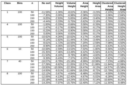
Table 1 displays the performance gap measures comparing the various heuristics using
the EPs and the CPs. The gaps were computed as (meanEP −meanCP)/meanCP ∗
100, where meanEP and meanCP were the mean values obtained by the given FFD
heuristics over 10 instances using the EPs and the CPs, respectively. A negative value
thus corresponds to better results of theEP-based version of the heuristics compared to
the results of the CP-based version. Column 1 gives the instance type, bin dimensions,
and the number of items. Column 2 presents the mean results when no sorting algorithm was used. Columns 3-6 present the mean results when height-volume, volume-height, area-height, and height-area sorting rules were used, respectively. The results of the clustered area-height and height-area sorting rules are reported in Columns 7 and 8, respectively. Computational times were negligible and, thus, are not reported.
The results displayed in Table 1 seem to indicate that usingEPs allows to better
ex-ploit the available volume of the bin and support the claim thatEP-based FFD heuristic
procedures are more efficient than CP-based ones. Differences in performance among
problem classes are mainly due to the different relationships between the dimensions of items and bins. When items are big, there are not many possibilities of placing them side
by side and, consequently, using EPs or CPs does not impact the performance so much.
The improvement yielded by using theEPs is more significant when the items are small
compared to the bin size. This is the case, for example, for Class V, which includes the instances considered as the most difficult to solve. Finally, notice that, when no initial ordering is imposed on the items, as in on-line packing problems, the number of bins can be reduced by up to 18%.
5.3 Comparing the different versions of the EP-FFD heuristic
We now present the results of extensive computational testing of the EP-FFD heuris-tics using different sorting rules. The issue of parameter tuning for best results is also addressed.
The results are summarized in Table 2, which columns have the same meaning as those of Table 1 and each value is the average result of ten instances belonging to the
same class. For each class of instances, the row Class total reports the number of bins
obtained as the sum of the results of the class instances. The last row of the table
displays the total number of bins used, computed as the sum of theClass total values in
the column. The results of the clustered area-height and height-area sorting rules were
obtained cycling on the same instance for all the values of the cluster size δ ∈ [1,100]
and considering the best solution among all theδvalues. Similarly to the previous set of
experiments, computational times are negligible and, thus, are not reported. In general,
EP-FFD runs in less than 10−2 seconds for the non-clustered versions and in less than
half a second for the clustered ones.
The experimental results indicate that the clustered area-height and the clustered
height-area are the best sorting rules. These rules are complementary, in the sense that they yield their best results on different instances, while outperforming the corresponding versions without clustering. This follows from the fact that the sorting rules without clustering introduce an ordering based mainly on the first parameter (e.g., the height in the height-area), neglecting the others. Clustering, on the other hand, allows to refine the order implied by the first criterion. Consider, for example, a set of items that are
Class Bins n No sort Height Volume Volume Height Area Height Height Area Clustered Area Height Clustered Height Area 1 100 50 14.6 15 14.4 14.4 15 14 13.8 100 29.2 29.2 29.5 28.3 29 27.9 27.4 150 40.1 39.9 40.3 39.2 39.8 38.1 37.7 200 55.9 55.6 55.7 53.2 55.1 53 52.3 139.8 139.7 139.9 135.1 138.9 133.0 131.2 4 100 50 29.7 30.1 29.9 30 30 29.5 29.5 100 60.2 59.6 60.4 59.7 59.6 59 59 150 88.5 88.3 88.6 88.4 88.3 86.9 86.9 200 119.9 120.1 119.6 120.3 120 119 118.9 298.3 298.1 298.5 298.4 297.9 294.4 294.3 5 100 50 10.1 9 10 9.2 9 8.5 8.4 100 18.1 16.7 17.8 16.1 16.6 15.7 15.4 150 24.4 22.9 24.5 21.9 22.6 21 21.1 200 32.5 30.7 32.6 29.5 30.5 28.5 28.2 85.1 79.3 84.9 76.7 78.7 73.7 73.1 6 10 50 11.7 10.9 11.7 10.6 10.9 10.2 10.1 100 21.7 21.2 22 20.2 20.5 19.6 19.8 150 33 31.8 34.2 30.8 31 29.9 30.2 200 44.4 41.5 44 39.5 39.8 38.6 38.8 110.8 105.4 111.9 101.1 102.2 98.3 98.9 7 40 50 9.4 8.2 9.3 8.1 8.1 7.6 7.7 100 15.9 14.6 15.6 14.1 14.1 13.4 13.3 150 19.3 19.2 19.7 18.2 18.9 16.9 16.9 200 30 28.1 30.2 26.2 27.2 25 24.9 74.6 70.1 74.8 66.6 68.3 62.9 62.8 8 100 50 11.6 10.5 11.6 10.1 10.5 9.6 9.5 100 22 20.9 22.1 20.3 20.8 19.4 19.7 150 28.5 27.4 28.4 26.4 27.7 25.4 25.5 200 35.4 33.9 35.4 32.2 33.9 31.4 31.5 97.5 92.7 97.5 89.0 92.9 85.8 86.2 806.1 785.3 807.5 766.9 778.9 748.1 746.5 Total Class total Class total Class total Class total Class total Class total
Table 2: Results of the EP-FFD Heuristic
equal in height but have different base areas. The height-area sorting rule would pack all these items together even though they are dissimilar in base area. The clustered version avoids this situation by using the second sorting parameter to build more homogeneous packings of items that are almost equal in height and have similar base areas.
3D_FFD_results_AZD.png
Figure 7: Total Number of Bins versus δ: Clustered Area-Height with the EP-FFD
Heuristic
Clustered area-height and height-area sorting rules require tuning the δ parameter.
Figures 7 and 8 display the results of the EP-FFD heuristic with the clustered
area-height and clustered area-height-area sorting rules, respectively, for varying values of δ. In
both graphs, the horizontal axis represents theδvalues, while the sum of the bins built for all 240 benchmark instances is mapped on the vertical axis. The results indicate that the
3D_FFD_results_ZAD.png
Figure 8: Total Number of Bins versus δ: Clustered Height-Area with the EP-FFD
Heuristic
EP-FFD heuristic with clustered area-height obtains its best results forδ ∈[5,25], while
the EP-FFD procedure with clustered height-area has two optimality regions, one around
δ = 20 and the other aroundδ= 55. On the other hand, EP-FFD performs poorly when
δ is greater than 60, independently of the sorting rule. This is not surprising considering
that, for δ >50, the clustering splits the items into two clusters only. Moreover, while
δ is increasing, the number of items in the first cluster increases and the sorting mainly
applies the secondary rule.
The average values displayed in Table 2 seem to indicate that a better performance could be achieved by taking the best of the results obtained by the EP-FFD heuristic with Clustered Area-Height and with Clustered Height-Area. This is not true in general, as the comparison of the results instance by instance can demonstrate. Yet, this approach offers the best compromise between accuracy and computation effort and should be used.
5.4 Comparing the different versions of the EP-BFD heuristic
We now turn to the results of the extensive computational experiments of the 28 versions
of the EP-BFD heuristic. These variants are obtained combining the merit functions of
Section 4.3 with and without the various item sorting rules.
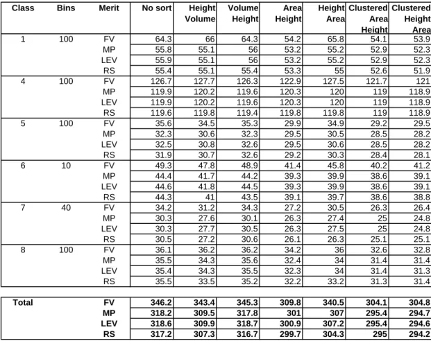
The general trends are illustrated by the results obtained on instances with 200 items displayed in Table 3, which columns have the same meaning as those of Table 1. Given an instance class, each row reports the results obtained by means of FV, MP, LV, and
RS merit functions. The row Total displays, for each combination of merit function
and sorting rule, the total number of bins obtained as the sum of the results of the class instances for that combination. Each value is the average result of ten instances belonging to the same class. The results of the clustered area-height and height-area
sorting rules were obtained cycling on the same instance for all the values of δ∈[1,100]
and considering the best solution among all theδvalues. Similarly to the previous set of
experiments, computational times are negligible and, thus, are not reported. In general,
EP-BFD runs in less than 10−2 seconds for the non-clustered versions and in less than
Class Bins Merit No sort Height Volume Volume Height Area Height Height Area Clustered Area Height Clustered Height Area 1 100 FV 64.3 66 64.3 54.2 65.8 54.1 53.9 MP 55.8 55.1 56 53.2 55.2 52.9 52.3 LEV 55.9 55.1 56 53.2 55.2 52.9 52.3 RS 55.4 55.1 55.4 53.3 55 52.6 51.9 4 100 FV 126.7 127.7 126.3 122.9 127.5 121.7 121 MP 119.9 120.2 119.6 120.3 120 119 118.9 LEV 119.9 120.2 119.6 120.3 120 119 118.9 RS 119.6 119.8 119.4 119.8 119.8 119 118.9 5 100 FV 35.6 34.5 35.3 29.9 34.9 29.2 29.5 MP 32.3 30.6 32.3 29.5 30.5 28.5 28.2 LEV 32.5 30.8 32.6 29.5 30.6 28.5 28.2 RS 31.9 30.7 32.6 29.2 30.3 28.4 28.1 6 10 FV 49.3 47.8 48.9 41.4 45.8 40.2 41.2 MP 44.4 41.7 44.2 39.3 39.9 38.6 39.1 LEV 44.6 41.8 44.5 39.3 39.9 38.6 39.1 RS 44.3 41 43.5 39.1 39.7 38.6 38.8 7 40 FV 34.2 31.2 34.3 27.2 30.5 26.3 26.4 MP 30.3 27.6 30.1 26.3 27.4 25 24.8 LEV 30.3 27.7 30.5 26.3 27.5 25 24.8 RS 30.5 27.2 30.6 26.1 26.3 25.1 25.1 8 100 FV 36.1 36.2 36.2 34.2 36 32.6 32.8 MP 35.5 34.3 35.6 32.4 34 31.4 31.4 LEV 35.4 34.3 35.5 32.3 34 31.4 31.3 RS 35.5 33.5 35.2 32.2 33.2 31.3 31.4 Total FV 346.2 343.4 345.3 309.8 340.5 304.1 304.8 MP 318.2 309.5 317.8 301 307 295.4 294.7 LEV 318.6 309.9 318.7 300.9 307.2 295.4 294.6 RS 317.2 307.3 316.7 299.7 304.3 295 294.2
The experimental results indicate that the EP-BFD heuristic providing the best
re-sults is using the Residual Space criterion. Indeed, using this criterion, one emulates
best the mono-dimensional BFD heuristics. Consider the Residual Space of each EP as
a “virtual bin”. Placing each item on theEP for which the difference between its
dimen-sions and theRS is minimal, we reduce the waste of space resulting from the splitting of
the bin volume due to the loading of the item. On the other hand, the minimization of the free volume, which seems to exactly reproduce the rule applied in mono-dimensional bin packing, yields results which are far from those of the EP-FFD procedure.
3D_RSPACE_results_AZD.png
Figure 9: Total Number of Bins versusδ: EP-BFD Heuristic with Clustered Area-Height
3D_RSPACE_results_ZAD.png
Figure 10: Total Number of Bins versus δ: EP-BFD Heuristic with Clustered
Height-Area
Similarly to the calibration of the EP-FFD heuristic and in order to reduce the
number of iterations, we analyzed the behavior of the EP-BFD heuristic relative to theδ
parameter. Given the results presented earlier in this section, we focused on the variants with Residual Space merit function and Clustered Area-Height and Clustered
Height-Area sorting rules. For the former, best results were obtained for δ ∈[5,15], while the
latter had two optimality regions, one at δ ∈ [21,24] and another at δ ∈ [50,57]. In
both cases, and for the same reasons indicated for the EP-FFD heuristic, the EP-BFD
where the values of δ are on the horizontal axis, while the vertical axis corresponds to the values of the sum of the bins built for all 240 benchmark instances.
The versions of the EP-BFD heuristic with clustered item sorting rules outperform on average the corresponding versions without clustering. This is similar to the performance of the EP-FFD heuristic. Unlike the latter, however, the EP-BFD heuristic with clustered sorting and Residual Space merit function yields also the best results, compared to unclustered versions, when considering the single problem instances from each class. It is not possible, however, to establish a clear dominance between the two clustered versions. Finally, comparing the FFD and BFD approaches based on the mean results, one observes a small gap between the EP-FFD heuristic and the EP-BFD procedure with Residual Space.
Class Bins n C-EPBFD Score S-PACK MPV-BS HA MPV 1000 sec GLS 1000 sec LB Gap MPV 1000 sec Gap GLS 1000 sec Gap LB 1 100 50 13.7 15.3 13.5 13.9 13.6 13.4 12.9 0.74% 2.24% 6.20% 100 27.2 27.4 29.5 27.6 27.3 26.7 25.6 -0.37% 1.87% 6.25% 150 37.7 40.4 38 38.1 38.2 37 35.8 -1.31% 1.89% 5.31% 200 51.9 55.6 52.3 52.7 52.3 51.2 49.7 -0.76% 1.37% 4.43% 130.5 138.7 133.3 132.3 131.4 128.3 124.0 4 100 50 29.4 29.8 29.4 29.4 29.4 29.4 29 0.00% 0.00% 1.38% 100 59 60 59 59 59.1 59 58.5 -0.17% 0.00% 0.85% 150 86.8 87.9 87.3 86.9 87.2 86.8 86.4 -0.46% 0.00% 0.46% 200 118.8 120.3 119.3 119 119.5 119 118.3 -0.59% -0.17% 0.42% 294.0 298.0 295.0 294.3 295.2 294.2 292.2 5 100 50 8.4 10.2 9.1 8.5 9.2 8.3 7.6 -8.70% 1.20% 10.53% 100 15.1 17.6 17 15.1 17.5 15.1 14 -13.71% 0.00% 7.86% 150 21 24 23.7 21.4 24 20.2 18.8 -12.50% 3.96% 11.70% 200 28.1 31.7 31.7 28.6 31.8 27.2 26 -11.64% 3.31% 8.08% 72.6 83.5 81.5 73.6 82.5 70.8 66.4 6 10 50 10.1 11.2 11 10.5 9.8 9.8 9.4 3.06% 3.06% 7.45% 100 19.6 24.5 22.3 20 19.4 19.1 18.4 1.03% 2.62% 6.52% 150 29.9 35 32.4 30.6 29.6 29.4 28.5 1.01% 1.70% 4.91% 200 38.5 42.3 40.8 39.1 38.2 37.7 36.7 0.79% 2.12% 4.90% 98.1 113.0 106.5 100.2 97.0 96.0 93.0 7 40 50 7.5 9.3 8.2 8 8.2 7.4 6.8 -8.54% 1.35% 10.29% 100 13.2 15.3 13.9 13.3 15.3 12.3 11.5 -13.73% 7.32% 14.78% 150 17 20.1 18.1 17.2 19.7 15.8 14.4 -13.71% 7.59% 18.06% 200 25.1 28.7 28 25.2 28.1 23.5 22.7 -10.68% 6.81% 10.57% 62.8 73.4 68.2 63.7 71.3 59.0 55.4 8 100 50 9.4 11.3 9.9 9.9 10.1 9.2 8.7 -6.93% 2.17% 8.05% 100 19.5 21.7 20.2 19.9 20.2 18.9 18.4 -3.47% 3.17% 5.98% 150 25.2 28.3 26.8 25.7 27.3 23.9 22.5 -7.69% 5.44% 12.00% 200 31.3 35 34 31.6 34.9 29.9 28.2 -10.32% 4.68% 10.99% 85.4 96.3 90.9 87.1 92.5 81.9 77.8 743.4 802.9 775.4 751.2 769.9 730.2 708.8 Class total Class total Total Class total Class total Class total Class total
Table 4: C-EPBFD versus State-of-the-art Algorithms for the3D-BP Problem
5.5 Results for the composite heuristics
Let’s define two composite heuristics. The first, identified as C-EPFFD, applies
succes-sively the EP-FFD heuristic with the two clustered sorting rules, cycling on the different
values ofδ, and selects the best result. The second is identified as C-EPBFD and follows
the same procedure using the EP-BFD heuristic. The results displayed in the previ-ous tables provide the means to evaluate the relative performance of the two composite heuristics and show that C-EPBFD is always able to find solutions at least as good as
those obtained by C-EPFFD. We therefore retain the C-EPBFD composite heuristics to
Class Bins n FBL FFF FBF AD FC KP HBM Best Best Bound 1 10 20 -16.47% -13.41% -6.58% -26.80% -21.98% -16.47% -16.47% 0.00% 0.00% 40 2.26% -9.93% -8.11% -8.11% -2.16% 2.26% 1.49% 2.26% 3.82% 60 -0.98% -9.01% -9.42% -11.40% -4.72% -1.46% 0.50% 0.50% 2.54% 80 -5.48% -6.76% -8.31% -6.44% -4.50% -3.83% 0.73% 0.73% 0.73% 100 -4.14% -4.14% -8.47% -3.57% -2.41% -1.82% 1.25% 1.89% 2.21% -4.09% -7.35% -8.44% -8.61% -5.08% -2.98% -0.49% 1.20% 1.92% 2 30 20 -52.38% -9.09% -50.00% -50.00% -66.67% -67.74% -67.74% 0.00% 0.00% 40 0.00% 0.00% -37.50% 0.00% 0.00% 0.00% 5.26% 5.26% 5.26% 60 -10.34% -10.34% -48.00% -3.70% -10.34% -10.34% 4.00% 4.00% 4.00% 80 6.45% -2.94% -52.17% -2.94% -2.94% -2.94% 3.12% 6.45% 6.45% 100 2.56% 0.00% -54.02% 0.00% 0.00% 0.00% 2.56% 2.56% 2.56% -7.86% -3.73% -50.00% -8.51% -15.69% -16.23% -11.64% 4.03% 4.03% 3 40 20 -7.02% -11.67% -8.62% -11.67% -11.67% -7.02% -3.64% 3.92% 3.92% 40 2.11% -9.35% -11.01% -5.83% -2.02% 4.30% 2.11% 4.30% 5.43% 60 -4.05% -12.35% -14.97% -11.80% -2.74% -2.07% -2.74% 1.43% 4.41% 80 -7.08% -10.45% -13.97% -10.45% -2.48% -2.96% 4.23% 4.23% 5.35% 100 -7.26% -9.09% -13.21% -10.16% -2.95% -2.95% 2.22% 2.22% 4.07% -5.39% -10.35% -13.16% -10.13% -3.36% -2.18% 1.27% 3.01% 4.66% 4 100 20 -23.08% 0.00% -44.44% -56.52% -54.55% -28.57% -28.57% 0.00% 0.00% 40 -93.33% 0.00% -33.33% 5.26% -93.33% -93.33% -93.10% 5.26% 5.26% 60 -69.05% -3.70% -43.48% -7.14% -69.05% -69.05% -68.29% 4.00% 13.04% 80 -2.94% 0.00% -46.77% -5.71% -2.94% -2.94% 0.00% 3.12% 10.00% 100 5.00% 5.00% -48.15% 10.53% 5.00% 5.00% 5.00% 10.53% 13.51% -72.19% 0.77% -44.73% -8.39% -72.71% -72.25% -71.46% 5.65% 10.08% 5 100 20 -4.41% -2.99% -5.80% -4.41% -4.41% -4.41% 0.00% 0.00% 0.00% 40 1.68% -7.63% -7.63% -9.70% -4.72% 0.00% 1.68% 1.68% 4.31% 60 -5.70% -7.14% -6.67% -6.67% -4.21% -1.09% 0.55% 1.11% 1.68% 80 -5.66% -9.75% -11.66% -16.11% -2.72% -2.34% 1.21% 1.21% 3.73% 100 -3.02% -10.53% -11.89% -12.69% -2.69% -2.36% 3.58% 3.58% 3.58% -3.82% -8.75% -9.84% -11.60% -3.41% -1.95% 1.80% 1.91% 3.07% 6 300 20 -96.55% 0.00% -44.44% -97.22% -97.22% -97.14% -96.43% 0.00% 0.00% 40 -59.57% 0.00% -32.14% -64.81% -64.81% -64.15% -56.82% 11.76% 26.67% 60 -23.33% 4.55% -47.73% -23.33% -23.33% -23.33% 9.52% 9.52% 9.52% 80 0.00% 0.00% -48.28% 0.00% 0.00% 0.00% 0.00% 0.00% 0.00% 100 -7.69% 2.86% -50.68% -2.70% -7.69% -7.69% -5.26% 5.88% 12.50% -72.94% 1.72% -46.61% -76.91% -77.00% -76.49% -71.43% 5.36% 9.26% 7 100 20 -3.45% -11.11% -3.45% -12.50% -11.11% -6.67% 0.00% 1.82% 1.82% 40 -0.88% -6.61% -5.04% -6.61% -4.24% 0.89% 0.89% 1.80% 3.67% 60 -7.47% -8.52% -9.55% -11.05% -6.40% -4.17% -3.01% 0.63% 3.21% 80 -3.33% -9.73% -10.77% -13.43% -1.69% -1.69% 1.75% 1.75% 3.57% 100 -3.17% -7.09% -6.78% -8.33% -2.14% -1.79% -1.08% 0.36% 2.23% -3.79% -8.32% -8.02% -10.39% -3.79% -2.22% -0.36% 1.09% 2.95% 8 100 20 -47.32% -7.81% -1.67% -6.35% -48.25% -47.32% -43.27% 1.72% 1.72% 40 -0.86% -7.26% -3.36% -8.00% -10.16% -3.36% -4.17% 1.77% 2.68% 60 0.62% -6.86% -6.86% -11.89% -4.12% -2.40% 0.62% 0.62% 2.52% 80 -1.30% -6.58% -6.20% -8.10% -2.99% -0.87% 0.44% 0.89% 1.79% 100 -3.45% -8.79% -7.89% -11.67% -2.78% -0.71% -2.44% 0.00% 2.19% -7.25% -7.56% -6.22% -9.93% -9.64% -7.15% -6.12% 0.72% 2.18% 9 100 20 -57.94% -60.28% 0.00% -64.25% -57.94% -56.67% -56.67% 0.00% 0.00% 40 -10.61% -15.24% 0.00% -20.11% -12.58% -9.15% -15.76% 0.00% 0.00% 60 -0.91% -5.21% 0.00% -5.21% -5.21% -0.91% -0.46% 0.00% 0.00% 80 0.00% 0.00% 0.00% 0.00% 0.00% 0.00% 0.00% 0.00% 0.00% 100 -3.47% -4.53% 0.00% -4.53% -4.53% -3.47% -1.00% 0.00% 0.00% -10.84% -13.20% 0.00% -15.27% -12.13% -10.28% -10.43% 0.00% 0.00% 10 100 20 -76.50% -15.69% -14.00% -10.42% -76.50% -76.50% -84.25% 0.00% 2.38% 40 -1.33% -13.95% -19.57% -8.64% -5.13% -2.63% -2.63% 0.00% 0.00% 60 -5.41% -13.93% -23.91% -13.22% -4.55% -5.41% -4.55% 1.94% 7.14% 80 -3.62% -17.39% -21.30% -18.40% -2.21% -2.92% 2.31% 2.31% 8.13% 100 -3.53% -14.58% -21.53% -13.68% -1.80% -0.61% 1.86% 1.86% 7.19% -23.34% -15.20% -21.12% -13.93% -23.00% -22.77% -30.80% 1.57% 5.92% -14.75% -9.78% -10.57% -15.79% -16.24% -14.69% -12.82% 1.24% 2.33% Class total Class total Total Class total Class total Class total Class total Class total Class total Class total Class total
Table 5: Percentage comparison of the C-EPBFD versus State-of-the-art Heuristics for the2D-BP Problem (in %)
5.6 The C-EPBFD heuristic versus state-of-the-art algorithms
We compared the performances of the C-EPBFD heuristic to those of the other con-structive heuristics presented in Section 2, as well as to those of more complex solution methods, meta-heuristics and Branch & Bound-based algorithms. We also applied the
C-EPBFD heuristic to the 2D-BP problem and compared its performance to that of the
constructive heuristics developed explicitly for the2D-BP problem.
Algorithms GLS (Faroe et al. 2003) and HA (Lodi et al. 2002b) were coded
in C and run on a Digital 500 workstation with a 500 MHz CPU. Algorithms S-Pack,
MPV-BS, andM P V (Martello et al. 2000) were coded in C and tested on a Pentium4
2000 MHz CPU. For M P V a time limit of 1000 seconds was imposed for each instance.
The results of GLS are taken from the literature and were obtained with a time limit
of 1000 seconds for each instance on a Digital 500 workstation CPU (equivalent to 300 seconds on the Pentium4 2000 MHz CPU, according to the SPEC CPU2000 benchmarks published in (Standard Performance Evaluation Corporation ????) ).
The results for the three-dimensional case are summarized in Table 4. The instance type, bin dimensions, and the number of items are given in the first column, while the second displays the mean results of the C-EPBFD heuristic. The mean results obtained
by the S-Pack (Martello et al. 2000) ,MPV-BS (Martello et al. 2000) , and HA (Lodi
et al. 2002b) constructive heuristics are displayed in columns 3, 4, and 5, respectively,
while columns 6, 7, and 8 display, respectively, the results obtained byMPV, theBranch
and Bound proposed by Martello, Pisinger, and Vigo (Martello et al. 2000) ,GLS, the meta-heuristic algorithm by Faroe, Pisinger, and Zachariasen (Faroe et al. 2003) , and
LB, the lower bound proposed by Boschetti (Boschetti 2004) . Finally, columns 9, 10,
and 11 display the gaps of the mean solutions obtained by C-EPBFD relative to those of M P V, GLS, and LB, respectively. The gaps were computed as (meanC−EP BF D− meano)/meano, where, for a given set of problem instances,meanC−EP BF D and meano are the mean values obtained by the C-EPBFD heuristics and the method compared to, respectively. A negative value signals that C-EPBFD yielded a better mean value. For
each class of instances, the row Class total reports the number of bins obtained as the
sum of the results of the class instances. The last row of the table displays the total
number of bins used, computed as the sum of theClass total values in the column.
These results show that C-EPBFD achieves better results than the other constructive
heuristics. Moreover, it also obtains better results than those of the Branch and Bound
M P V. The GLS meta-heuristic algorithm obtains better results than our method but the gaps are less than 2% with a computational effort of half a second in the worst case
against 1000 seconds needed by MPV and GLS. Furthermore, the gaps between the
lower bound and the results of our method are quite small (less than 5%). In particular in Class IV, the gap is less than 1%. This is the class where the majority of the items are bigger than half bin, so the value of the lower bound is tight to the optimal one
and, in Class IV, C-EPBFD improves the results ofGLS. This performance is the more
remarkable given that the C-EPBFD solutions were obtained within a computational
effort three orders of magnitude smaller than both MPV and GLS.
The C-EPBFD heuristic was tested also on 2D-BP problem instances. The
re-sults are summarized in Table 5 as relative gaps, in %, between the C-EPBFD
com-puted as (meanC−EP BF D−meano)/meano where, for a given set of problem instances,
meanC−EP BF D and meano represent the mean values obtained by C-EPBFD and the
method it is compared to, respectively. A negative value signals a better performance of the C-EPBFD heuristic. The instance type, bin dimensions, and the number of items are given in the first column, while columns 2 to 8 present the results for the constructive heuristics in the literature (see (Monaci and Toth 2006) for a detailed presentation of the heuristics):
• Greedy procedures:
– Finite Bottom Left(FBL),Finite First Fit (FFF), andFinite Best Fit (FBF), proposed by Berkey and Wang (Berkey and Wang 1987) ;
– Alternate Directions (AD), proposed by Lodi, Martello, and Vigo (Lodi et al. 1999b) .
• Constructive heuristics
– Floor Ceiling (FC) andKnapsack Packing (KP), proposed by Lodi, Martello, and Vigo (Lodi et al. 1999a,b) ;
– HBM, proposed by Boschetti and Mingozzi (Boschetti and Mingozzi 2003) ,
limited to 250 iterations.
All the heuristics were coded in Fortran (Monaci and Toth 2006) . Column 9 (Best)
displays the minimum value of the results of the seven heuristics, while column 10 presents
the value of the best lower bound. For each class of instances, the row Class total
reports the overall class performances, while the rowTotal displays the performances by
considering the bins used in the total number of instances.
The figures displayed in Table 5 show that these best heuristics for the2D-BP
prob-lem present a high variability of results relative to the probprob-lem class. To obtain more stable results, the seven heuristics must be executed and the best result chosen (column 9). Compared to each of the seven heuristics individually, the C-EPBFD heuristic builds the minimum number of bins, decreasing the total number of bins between 9 and 15%. Even when compared to the composite heuristic that takes the best solution of the seven heuristics, the performance is impressive, the gap being around 1% only. And this is achieved without tailoring the method for 2D instances.
In the 2D case, the heuristic we propose is offering the best overall mean results when compared to each existing heuristics and is the only one that is effective for all the classes of test instances.
Thus, the C-EPBFD heuristic offers the best performance among existing heuristics
for both the 3D-BP and the 2D-BP problems. Moreover, it is comparable to more
computational expensive methods as Tabu Search, Branch & Bound and GLS.
6.
Conclusions
We introduced the Extreme Points, a new definition for the points where to place an
item in a three-dimensional container, and applied this idea to the3D-BP problem. The
volumes compared to the definitions currently used in the literature. We also derived a new heuristic algorithm, called C-EPBFD, which integrates the Extreme Point placement concept. Extensive experimental results indicate that the C-EPBFD algorithm requires negligible computational efforts and yields better results compared not only to all
exist-ing constructive heuristics for the 3D-BP problem, but also to more complex methods
such as the Branch & Bound by Martello, Pisinger, and Vigo (Martello et al. 2000) .
Moreover, the same algorithm applied to the 2D-BP problem yields results that
outper-form those of the existing constructive heuristics. Thus, C-EPBFD can be considered as the current best constructive heuristics for the multi-dimensional Bin Packing problem. Notice, finally, that item rotation can be easily introduced in the proposed algorithms by duplicating each item once for each possible rotation and adding a constraint on the mutual exclusion of the duplicates. This would imply small changes in the code without additional computational effort.
7.
Acknowledgments
This project has been partially supported by the Ministero dell’Universit`a e della Ricerca
(MUR), under the Progetto di Ricerca di Interesse Nazionale (PRIN) 2005 ”Sistemi di
Infomobilit`a e Distribuzione Merci in Aree Metropolitane” and by the Natural Sciences
and Engineering Research Council of Canada through its Discovery Research Grant program.
While working on this project, Prof. T.G. Crainic was Adjunct Professor at the D´epartement d’informatique et de recheche op´erationnelle of the Universit´e de Montr´eal, as well as at Molde University College, Molde, Norway.
The authors wish to thank Professor Paolo Toth and Dr. Michele Monaci for their
support and for providing their implementation of the 2D heuristics.
References
Baldacci, R., M. A. Boschetti. 2007. A cutting plane approach for the two-dimensional
orthogonal non guillotine cutting stock problem. European Journal of Operational
Research 1831136–1149. doi:10.1016/j.ejor.2005.11.060.
Beasley, J. E. 1985. An exact two-dimensional non-guillotine cutting stock tree search
procedure. Operations Research 3349–64.
Berkey, J. O., P. Y. Wang. 1987. Two dimensional finite bin packing algorithms. Journal
of the Operational Research Society 38423–429.
Boschetti, M. A. 2004. New lower bounds for the finite three-dimensional bin packing
problem. Discrete Applied Mathematics 140 241–258.
Boschetti, M. A., A. Mingozzi. 2003. The two-dimensional finite bin-packing problem.
part II: new lower and upper bounds. 4OR 1 135–147.
Chung, F. K. R., M. R. Garey, D. S. Johnson. 1982. On packing two-dimensional bins.
Crainic, T.G., G. Perboli, R. Tadei. forthcoming. TS2PACK: A two-stage tabu search
heuristic for the three-dimensional bin packing problem. European Journal of
Opera-tional Research .
den Boef, E., J. Korst, S. Martello, D. Pisinger, D. Vigo. 2005. Erratum to ”the three-dimensional bin packing problem”: Robot-packable and orthogonal variants of packing
problems. Operations Research 53735–736.
Faroe, O., D. Pisinger, M. Zachariasen. 2003. Guided local search for the
three-dimensional bin packing problem. INFORMS, Journal on Computing 15 267–283.
Fekete, S. P., J. Schepers. 1997. A new exact algorithm for general orthogonal
d-dimensional knapsack problems.ESA ’97, Springer Lecture Notes in Computer Science
1284144–156.
Fekete, S. P., J. Schepers. 2001. New classes of lower bounds for bin packing problems.
Mathematical Programming 91 11–31.
George, J. A., D. F. Robinson. 1980. A heuristic for packing boxes into a container.
Computers and Operations Research 7 147–156.
Gilmore, P. C., R. E. Gomory. 1965. Multistage cutting problems of two and more
dimensions. Operations Research 13 94–119.
Hadjiconstantinou, E., N. Christofides. 1995. An exact algorithm for general, orthogonal,
two-dimensional knapsack problems. European Journal of Operational Research 83
39–56.
Johnson, D. S. 1973. Near-optimal bin packing algorithms. Ph.D. thesis, Dept. of
Mathematics, M.I.T., Cambridge, MA.
Lodi, A., S. Martello, M. Monaci. 2002a. Two-dimensional packing problems: a survey.
European Journal of Operational Research 141241–252.
Lodi, A., S. Martello, D. Vigo. 1999a. Approximation algorithms for the oriented
two-dimensional bin packing problem. European Journal of Operational Research 112
158–166.
Lodi, A., S. Martello, D. Vigo. 1999b. Heuristic and metaheuristic approaches for a
class of two-dimensional bin packing problems. INFORMS Journal on Computing 11
345–357.
Lodi, A., S. Martello, D. Vigo. 2002b. Heuristic algorithms for the three-dimensional bin
packing problem. European Journal of Operational Research 141410–420.
Lodi, A., S. Martello, D. Vigo. 2004. Tspack: A unified tabu search code for
multi-dimensional bin packing problems. Annals of Operations Research 131203–213.
Martello, S., D. Pisinger, D. Vigo. 2000. The three-dimensional bin packing problem.