DigitalCommons@University of Nebraska - Lincoln
DigitalCommons@University of Nebraska - Lincoln
Computer Science and Engineering: Theses,Dissertations, and Student Research Computer Science and Engineering, Department of Fall 11-26-2013
Algorithms for Grid Graphs in the MapReduce Model
Algorithms for Grid Graphs in the MapReduce Model
Taylor P. SpanglerUniversity of Nebraska-Lincoln, [email protected]
Follow this and additional works at: https://digitalcommons.unl.edu/computerscidiss
Part of the Theory and Algorithms Commons
Spangler, Taylor P., "Algorithms for Grid Graphs in the MapReduce Model" (2013). Computer Science and Engineering: Theses, Dissertations, and Student Research. 66.
https://digitalcommons.unl.edu/computerscidiss/66
This Article is brought to you for free and open access by the Computer Science and Engineering, Department of at DigitalCommons@University of Nebraska - Lincoln. It has been accepted for inclusion in Computer Science and Engineering: Theses, Dissertations, and Student Research by an authorized administrator of
by
Taylor Spangler
A THESIS
Presented to the Faculty of
The Graduate College at the University of Nebraska In Partial Fulfilment of Requirements
For the Degree of Master of Science
Major: Computer Science
Under the Supervision of Professor Vinodchandran Variyam
Lincoln, Nebraska December, 2013
Taylor Spangler, M.S. University of Nebraska, 2013
Adviser: Vinodchandran Variyam
The MapReduce programming paradigm has seen widespread use in analyzing large data sets. Often these large data sets can be formulated as graphs. Many algorithms, such as filtering based algorithms, are designed to work efficiently for dense graphs - graphs with substantially more number of edges than the number of vertices. These algorithms are not optimized for sparse graphs - graphs where the number of edges is of the same order as the number of vertices. However, sparse graphs are also common in big data sets. In this thesis we present algorithms for maximal matching, approximate edge covering, and approximate maximum weighted matching problems over grid graphs, a natural class of sparse graphs -graphs where the vertices and edges lie on a two dimensional integer grid. These algorithms take advantage of the inherent structure of grid graphs, thus making them more efficient than the known algorithms. In addition, in the case of maximum weighted matching, the algorithm presented gives a better approximation ratio than previous MapReduce algorithms.
Contents
Contents iii
List of Figures v
1 Introduction 1
2 Background 4
2.1 Matchings and Coverings . . . 4
2.2 MapReduce . . . 5
2.3 Matrix Transpose in MapReduce . . . 6
2.4 Filtering Techniques . . . 7
2.4.1 Maximal Matching, a filtering example . . . 8
2.5 Bounds in MapReduce . . . 9
2.6 MRC . . . 10
2.7 DMRC . . . 11
2.8 Grid Graphs . . . 12
2.8.1 Grid Graph Representation in MapReduce . . . 12
3 Maximal Matching in Grid Graphs 14 3.1 Algorithm . . . 15
3.2 Correctness . . . 16 3.3 Efficiency . . . 19
4 Approximate Minimum Edge Covering in Grid Graphs 21
4.1 Algorithm . . . 21 4.2 Correctness . . . 22 4.3 Efficiency . . . 23
5 Approximate Maximum Weighted Matching in Grid Graphs 26
5.1 Algorithm . . . 26 5.2 Correctness . . . 27 5.3 Efficiency . . . 31 6 Conclusion 34 A MapReduce implementations 36 A.1 Hadoop . . . 36 A.2 MR-MPI . . . 37 A.3 Comparison . . . 38 Bibliography 39
List of Figures
2.1 Graph A is a grid graph. Graph B is not a grid graph. . . 12 3.1 This is blockB1,1for a 16×16 grid graph, where= 21. Here verticesv4, v8, v13, v14, v15,
and v16 are border vertices. The four corner vertices are: v1, v4, v13, and v16. Ad-ditionally, e1, e2, e3, e4, and e5 are cross edges. Notice that e12 is not a border vertex. . . 14
Chapter 1
Introduction
The amount of data being stored is growing at an exponential rate, approximately doubling every four years [7]. In many applications the data required to solve problems cannot fit on one machine, or even some small number of machines. Recently, new models of computation have been developed to facilitate more ways of solving problems on these large data sets.
One such new model for solving large problems is a distributed computation model called MapReduce [10]. The MapReduce computational model is based on a programming paradigm of the same name. This paradigm has seen widespread use in industry and was originally developed at Google [6]. The open source implementation, Hadoop [14], is an Apache product partially developed by Yahoo! and is used at Facebook for analyzing large data sets [3]. Hadoop has also seen use at many other companies and universities [10]. In MapReduce, the data is split among some number of machines and processed in parallel in one round. Next, the output of this round is remapped to some set of machines (which may or may not be the same as the previous round), sent to the new machines, and then processed in the next round. This is repeated until the problem is solved. The MapReduce computational model tries to capture the essence of the paradigm and allow mathematical analysis of problems and algorithms in this framework, by imposing restrictions on the machines used,
and mathematically describing the system.
Problems which are too large to be practically solved on one machine, or even a small number of machines, are commonly referred to as big data problems. Typically big data problems involve at least hundreds of gigabytes of data, but the size depends greatly on the application, the kinds of problems being solved, and the state of technology [9]. While there are many big data problems that fit well into the MapReduce model, one area that has seen lots of interest is massive graph problems. However, solving the problem is not the only concern. MapReduce rounds require lots of communication and shuffling of the data. In fact it is possible that the entire problem may be communicated to a new set of machines each round. This can be very time consuming, so limiting the number of rounds and the communication per round is desirable. Limiting the number of rounds required by an algorithm to a small constant number, say two or three, is the goal. There are probabilistic algorithms which solve maximal matching, approximate maximum weighted matching, minimum spanning tree, and approximate minimum edge cut in a constant number of rounds [12]. However, these algorithms were designed forc-dense graphs, that is, graphs withn nodes having at leastn1+c
edges. Therefore, these algorithms would not be efficient for sparse graphs. The techniques used to solve these problems in dense graphs involve shrinking the size of the problem by
filtering edges out of the graph, such that the filtered graph can fit on one machine. This is done repeatedly until the problem is solved. For sparse graphs, such as planar graphs, this technique does not typically work well. This is because these graphs have enough vertices that even performing computations with all of the vertices on one machine becomes impractical. Grid graphs are a family of sparse graphs, where each node lies on a grid, and the edges connect vertices which are one row or column away from each other. Here, grid graphs are explored in the context of MapReduce. Grid graphs have a structure that would appear to make them ideal candidates for the MapReduce computational model. In this thesis we investigate MapReduce algorithms for Grid graphs. First an overview of the MapReduce
computational model is introduced, followed by some definitions and known results for grid graphs. Finally, MapReduce algorithms for maximal matching, 32-approximation for minimum edge covering, and finally 12-approximation for maximum weighted matching in grid graphs are presented and analyzed. All three algorithms are shown to be deterministic, run in a constant number of MapReduce rounds, and to operate within the confines of the MapReduce model, when grid graphs contain O(nm) edges. This places maximal matching, 3
2-approximation for minimum edge covering, and 12-approximation for maximum weighted matching in the most efficient MapReduce classDMRC0 for grid graphs withO(nm) edges.
Chapter 2
Background
2.1
Matchings and Coverings
The algorithms presented in this thesis solve or approximate three fundamental problems in theoretical computer science. These problems are defined for an undirected graphG= (V, E), with vertex set V and edge setE, as follows:
Definition 2.1.1. We say that M ⊆E is a matching, if ∀e, f ∈M e is not adjacent to f. This matching is said to be maximal if every e∈E−M is adjacent to some f ∈M.
Definition 2.1.2. A matching M is a maximum cardinality matching, sometimes referred to as a maximum matching, if it is the matching of highest possible cardinality.
Definition 2.1.3. For a weighted graph G = (V, E), a matching M is a maximum weighted matching if there does not exist M0 on G, such that P
f∈M0w(f)>
P
e∈M w(e). Definition 2.1.4. A 12-approximation for maximum cardinality matching, M0 is a matching such that|M0| ≥ 1
2|M|where M is a maximum cardinality matching onG. Similarly
a 12-approximation for maximum weighted matching, M0, is a matching such that
P
f∈M0w(f)≥ 12
P
Definition 2.1.5. An edge cover on a graph G = (V, E) is a set of edges E0 ⊆ E, such that ∀v ∈V, ∃e ∈E0 where e is incident on v. A minimum edge coveris the edge cover of smallest cardinality.
Definition 2.1.6. A 32-approximation for minimum edge cover E0 is an edge cover on G such that |E0| ≤ 3
2|F| where F is a minimum edge cover on G
2.2
MapReduce
One of the primary programming paradigms used to handle problems with large amounts of data is the MapReduce paradigm. A MapReduce program consists of some finite number of MapReduce rounds. The input to each MapReduce round is a set of
hkey;valuei pairs, where the key and value are binary strings. Each round has three phases: a map phase, where eachsingle hkey;valuei pair is mapped to the machines in the system as a new multiset of hkey;valuei pairs where the values in each new hkey;valuei pair is a substring of the original value, a shuffle phasewhere the underlying system communicates thehkey;valueipairs to the machines as they were mapped, and a reduce phasewhere some function is computed on the data on each machine.
Definition 2.2.1. A mapper is a function (which may or may not be randomized) that receives one hkey;valuei pair as input. The mapper outputs a finite multiset of hkey;valuei
pairs.
Definition 2.2.2. A reducer is a function (which may or may not be randomized) that receives a key k, and a sequence of values v1, v2, ...all of which are binary strings. The reducer
outputs a multiset of pairs of binary strings hk;vk,1i, hk;vk,2i,.... The key in the output pairs
A MapReduce program consists of a finite sequence of MapReduce rounds,
hµ1, ρ1, µ2, ρ2, ...µR, ρRi, where eachµi is a mapper, each ρi is a reducer, and the subsequence hµi, ρiidenotes a MapReduce round. The input is a multiset of hkey;valueipairs, denoted by
U0, and Ui is the multiset of hkey;valuei pairs output by round i. The program executes as
follows:
For r= 1,2, ..., R:
1. Map: Feed each pairhk;viin Ur−1 to mapperµr and run it. The mapper will generate
a sequence of newhkey;valuei pairs hk1;v1i,hk2;v2i,.... Let Ur0 =∪hk;vi∈Ur−1µr(hk;vi)
2. Shuffle: For each k, let Vk,r be the values such that hk;vii ∈Ur0. Construct Vk,r from
Ur0.
3. Reduce: For each k, feed k and some arbitrary permutation of Vk,r to a separate
instance of reducer ρr and run it. The reducer will generate a sequence of tuples hk;v10i,hk;v20i,.... Let Ur be the multiset of hkey;valuei pairs output by ρr, that is,
Ur =∪kρr(hk;Vk,ri).
All following algorithms omit the shuffle phase, as the shuffle phase simply communicates the hkey;valuei pairs to the correct machines.
2.3
Matrix Transpose in MapReduce
Often MapReduce is used to solve problems that are very large, but simple in structure and easily parallelizable. An example of this would be transposing a matrix. A simple MapReduce algorithm for computing the transpose of a matrix can be seen as follows:
• Let the mappers each receive a hkey; valueisuch that the key is the row number i, and the value is the set of entries S = {mi,1, mi,2, ..., mi,n} in the given row of the n×n
matrix M.
Map: For each mi,j ∈S, construct the key/value pair hj; (mi,j, i)i.
Reduce: The reducers receive a key/value pair h j, S0 = {(mi1,j, i1),(mi2,j, i2), ...,(min,j, in)}i.
SortS0 on the ik term in each tuple (mik,j, ik). Output the new rowj of the transposed
matrix.
Here each ik is the row number associated with the given entry from M. However, the
shuffle phase does not guarantee that these are in any given order, therefore they must be sorted. Sorting them puts the entries in the order of the rows they originated from in M. And, because we used the column j as the key in the map phase, we know that eachmik,j
comes from column j. Thus, sorting the values in the reduce phase gives us the associated row in MT. Therefore, MT has been computed and can be output to a file, or used as part
of another MapReduce computation.
2.4
Filtering Techniques
One of the major challenges when working with MapReduce is that each machine can only work on a relatively small portion of the entire problem. In fact, the entire system only has enough space to store some constant number of copies of the entire problem. One way to handle this challenge is to construct a smaller version of the problem on one machine. This is typically referred to as filtering.
Filtering is a technique for designing algorithms, which has had some success on graph problems. Typically, when working with graphs, the filtering is done by repeatedly filtering a small number of edges from the entire graph onto one machine, and then constructing the
solution to the problem on this machine. This is repeated until the problem is solved, either approximately or exactly. This technique has been used to find a minimum spanning tree, maximal matching, 18-approximation for maximum weighted matching, minimum cut, and a
3
2-approximation for edge covering in a constant number of MapReduce rounds. The number of rounds for these algorithms is often parameterized with respect to the density of the graph, c, and the chosen , in the form bc
c. Because c≤2 and is constant, this leaves the number
of rounds constant. Parameterizing this way allows for a tradeoff between number of rounds, and the space required by each machine [12].
2.4.1
Maximal Matching, a filtering example
LetGbe a graph with nvertices and medges. Letµi denote mapperi, andρi denote reducer
i. A filtering algorithm for maximal matching essentially works as follows:
µ1: Map the graph to the MapReduce system, so that each machine has no more than
O(m1−) edges.
ρ1: Randomly sample edges by including each edge in the sample with probability p.
µ2: Remap all edges to the same key. Additionally, map all sampled edges to a new key.
ρ2: Construct a maximum matching on the sampled graph, and add it to the matching M.
µ3: Map all edges to the same key, additionally map M to every machine.
ρ3: Remove any edges adjacent to any matched edges in M. • Repeat until no edges remain.
This algorithm is probabilistic. The sampling probability pdoes not guarantee that only O(m1−) edges are sampled in total. However, it can be adjusted so that this algorithm is
The existing filtering algorithms are tailored to graphs where m ∈ O(n1+c). They are
less practical for sparse graphs. For example, in this maximal matching algorithm the entire partial matchingM is passed to every ρ3 by µ3. But M potentially has O(n) edges, and in a sparse graphm∈O(n). Therefore the size of the partial matching M is on the same order as the size of the entire problem. So, it would be impractical to pass the entire partial matching each round [12]. Thus, a different approach is needed for sparse graphs.
2.5
Bounds in MapReduce
The metrics typically used for efficiency in a MapReduce algorithm are the number of rounds required, and the amount of communication per round. There currently exist no lower bound techniques which can give lower bounds on the number of rounds for problems in the MapReduce model. However, research has been done on bounding the communication cost of problems in the MapReduce model, which require one or two rounds. This is done by modeling the tradeoff between parallelism and communication; more parallelization requires more communication.
The problems are viewed as sets of inputs, outputs, and a mapping of outputs to inputs. For example, finding the triangles in a graph: the inputs are sets of two nodes (edges), the outputs are sets of three nodes (the triangles), and the mapping from outputs to inputs is the set of three inputs representing the edges making up a given triangle. Hereq is defined as the maximum number of inputs a reducer can receive andr is the replication rate, or the number of key-value pairs that a mapper can create from each input. The parallelism/communication tradeoff can be seen here as smaller values of q require more machines to solve the problem, which leads to more communication.
The replication rate is used as a measure of the communication cost for an instance of the problem, and is defined in terms ofq and the size of the input. Among other results, the
upper and lower bound of r for finding the number of triangles in a graph of n nodes is √n
2q.
Similarly, the upper and lower bound of r for finding paths of length two in an n node graph is 2qn. The upper and lower bounds on r for matrix multiplication of an n×n matrix is 2nq2, however the upper bound only holds for q ≥2n2[1].
2.6
MRC
The definition for the MapReduce paradigm provides a good framework for parallelization. However, it does not lay any restrictions on the program, or provide any notion of efficiency. Thus, a MapReduce Class (MRC) must be defined to help classify problems and algorithms. Without a restriction on the amount of memory any machine is allowed, any problem with a polynomial time classical algorithm could be solved in one round. However, the reason to use MapReduce is that the problem can’t fit into the memory of one machine. Similarly, if any number of machines is allowed, the implementation becomes impractical. Lastly, some restriction must be placed on the amount of time that can be taken. For example, allowing any reducer to run in exponential time would not make practical sense. Similarly, shuffling is time consuming because communication is orders of magnitude slower than processor speeds. Thus the number of MapReduce rounds should be bounded in some way. These restrictions lead to the following definitions [10]:
Definition 2.6.1. A random access machine (RAM) consists of a finite program operating on an infinite sequence of registers, referred to as words[5].
Definition 2.6.2. Fix an >0. Let π be some arbitrary problem. We say π ∈ MRCi if there exists an algorithm that takes in a finite sequence of hkey; valuei pairs, hkj;vji such
that n = X
j
(|kj|+|vj|), and consists of a sequence hµ1, ρ1, µ2, ρ2, ..., µR, ρRi of operations
• Each µr is a randomized mapper implemented by a RAM with O(logn)-length words,
that uses O(n1−) space and polynomial time, with respect to n.
• Each ρr is a randomized reducer implemented by a RAM with O(logn)-length words,
that uses O(n1−) space and polynomial time, with respect to n. • The total space,Σhk;vi∈U0
r(|k|+|v|)used by thehkey;valueipairs output by µr isO(n
2−2). • The number of rounds R =O(login).
It is important to note that the space used by a RAM is measured by the number of words used. So, the definition above specifies that each mapper and reducer may use O(n1−)
words each of size O(logn).
2.7
DMRC
MRC is defined for randomized reducers and mappers. We can similarly define a deterministic MapReduce Class, DMRC as follows [10]:
Definition 2.7.1. Fix an >0. Let π be some arbitrary problem. We say π∈ DMRCi if
there exists an algorithm which takes in a finite sequence of hkey;valuei pairs, hkj;vji such
that n = X
j
(|kj|+|vj|), and consists of a sequence hµ1, ρ1, µ2, ρ2, ..., µR, ρRi of operations
which outputs the correct answer where:
• Each µr is a deterministic mapper implemented by a RAM with O(logn)-length words,
that uses O(n1−) space and polynomial time, with respect to n.
• Each ρr is a deterministic reducer implemented by a RAM with O(logn)-length words,
that uses O(n1−) space and polynomial time, with respect to n. • The total space,Σhk;vi∈U0
r(|k|+|v|)used by thehkey;valueipairs output by µr isO(n
• The number of rounds R =O(login).
Because the shuffle phase is so time consuming, the goal when designing MapReduce algo-rithms is O(1) rounds, typically a small constant. Even O(logn) rounds is often impractical. Thus, algorithms in MRC0 and DMRC0 are desired if possible.
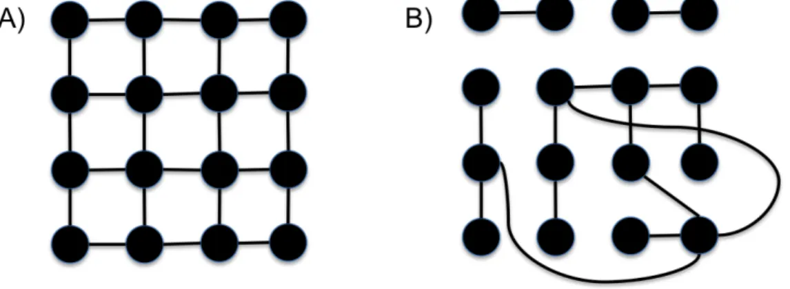
Figure 2.1: Graph A is a grid graph. Graph B is not a grid graph.
2.8
Grid Graphs
A grid graph is defined as a node-induced subgraph of the two-dimensional integer grid, that is, a graph where each vertex corresponds to some point (x, y), where x, y ∈Z. Each vertex v = (x, y) can be adjacent to at most four other vertices (x+ 1, y),(x, y+ 1),(x−1, y), and (x, y−1).
2.8.1
Grid Graph Representation in MapReduce
In the MapReduce model, the basic unit of information is the hkey;valueipair. It is important that grid graphs be defined in terms of the MapReduce model, so that the algorithms presented here may be analyzed in terms of this model. Here thevalue in eachhkey;valuei
by a list of edges of the form ((x1, y1),(x2, y2), w), where (xi, yi) is the point on the grid on
which the vertex lies, and w is the weight of the edge. In the case of unweighted graphs, the weight is omitted. The length of a value, then, is the number of edges listed plus one. The
key in each hkey;valuei pair represents the grouping of the edges. The initial input to the first map round may not have a meaningful key. However, the map functions presented here are all deterministic, thus after the first round the key has meaning. For example, many of the algorithms presented here, for grid graphs, map the edges to n1−×m1− blocks of the
original grid graph. Thus the key would indicate the block assigned to the machine. The length of the key is simply one. The space used by a hkey;valuei pair is defined as the length of the pair [10]. Therefore, the space of a hkey;valuei pair is the number of edges in the
value plus two. So, because the total number of machines is equal to the number of distinct keys and each machine can only storeO(|E|1−) edges, the total space required by all of the hkey;valuei pairs for a grid graph is O(|E|+|E|) which is O(|E|) when <1.
Chapter 3
Maximal Matching in Grid Graphs
One elementary graph problem is the maximal matching problem. This is often used as a 1
2-approximation for maximum cardinality matching. This algorithm works by constructing a maximum matching on the portion of the graph stored on each machine, and then attempt-ing to match any unmatched vertices by sharattempt-ing open edges with machines that contain neighboring vertices.
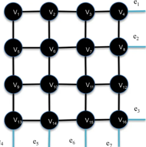
Figure 3.1: This is block B1,1 for a 16×16 grid graph, where = 12. Here vertices
v4, v8, v13, v14, v15, and v16 are border vertices. The four corner vertices are: v1, v4, v13, and v16. Additionally, e1, e2, e3, e4, and e5 are cross edges. Notice that e12 is not a border vertex.
Definition 3.0.1. For an grid graph G with lying on ann×m grid, and fixed >0, a block
Bi,j ⊆G is the subgraph containing all of the vertices in rows (i∗n1−) + 1 to (i+ 1)∗n1−,
and columns (j∗m1−) + 1 to (j+ 1)∗m1−.
Definition 3.0.2. An edge e= (u, v) is called a cross edge ifu∈Bi,j and v ∈Bi0,j0, where
i6=i0 and j 6=j0.
Definition 3.0.3. A vertex is called a border vertex, if it is incident on a cross edge.
Definition 3.0.4. A vertex, v = (x, y), is called a corner vertex when v ∈Bi,j, and v is one
of {((i∗n1−) + 1,(j ∗m1−) + 1,((i∗n1−) + 1,(j + 1)∗m1−),((i+ 1)∗n1−,(j∗m1−) + 1),((i+ 1)∗n1−,(j+ 1)∗m1−)}.
3.1
Algorithm
Given a grid graph G lying on ann×m grid, such that V(G)⊆ {(x, y)|1≤x≤n and 1≤
y ≤ m}. Let µi denote mapper i, and ρi denote reducer i. A maximal matching can be
constructed using the MapReduce paradigm as follows:
µ1: Map the grid graph to theO(nm) machines such that each machine gets edges incident on vertices that lie on a block of the original grid, with n1−m1− points, where the
block, Bi,j, will get the edges incident on vertices in the columns (i∗n1−) + 1 through
(i+ 1)∗n1−, and the rows (j∗m1−) + 1 through (j+ 1)∗m1−. Additionally, map
edges incident on corner vertices of each Bi,j, to Bi,j+1, Bi+1,j, Bi+1,j+1.
ρ1: Construct a maximum cardinality matching on the block Bi,j, using the Hopcroft-Karp
algorithm [8], ignoring any cross edges.
µ2: Map the matching for block Bi,j, called Mi,j, to the same key asBi,j. Map any cross
unmatched vertex (e.g. for edge e = (u, v) where u ∈ Bi,j and v ∈ Bi,j+1, where u is unmatched; map edge e to Bi,j and to Bi,j+1). For corner vertices, map the cross edges that are unmatched to all four blocks bordering the corner vertex the cross edge is associated with (e.g. for the edge e = (u, v) ∈ Bi,j, where u is the vertex
((i+ 1)∗n1−,(j+ 1)∗m1−), pass the edge toBi,j, Bi+1,j, Bi,j+1, and Bi+1,j+1).
ρ2: For each Mi,j, extend the matching to use any cross edges, where two copies of the edge
are available. For corner vertices, check all four edges for a given corner and match edges as follows:
1. If all four edges have two copies, choose the horizontal edges.
2. If three edges have two copies, choose the two that would lead to the largest valid matching.
3. If two edges have two copies, and they are not adjacent, pick both.
4. If two edges have two copies, and they are adjacent, choose the horizontal edge. 5. If one edge has two copies, match that edge.
6. If no edges have two copies, do not extend the matching.
3.2
Correctness
The algorithm results in a maximal matching on the original grid graph. To prove this, first observe the following lemma:
Lemma 3.2.1. After the first MapReduce round of the algorithm, the only way the partial matching can be extended is by matching on cross edges.
Proof. Suppose after round one, there exists some edge, e ∈ Bi,j, that is not a cross edge
contradiction, since the first round would have matched u and v on edge e. Therefore after round one, any unmatched vertex can only be matched with a cross edge.
Theorem 3.2.2. The algorithm constructs a maximal matching on the original grid graph,
G.
Proof. Clearly, grid graphs are bipartite. Therefore, by the properties of the Hopcroft-Karp algorithm [8], after round one of this algorithm each block, Bi,j, is maximally matched.
Because of the structure of grid graphs, the only vertices incident on cross edges in blockBi,j
are those in column i∗n1−, those in column (i+ 1)∗n1−, those in rowj∗m1−, or those in
row (j+ 1)∗m1− (the first column, last column, first row, or last row of each block). Notice
that each corner vertex is incident on at most two cross edges. In round two, all blocks are remapped to the same key. However, all cross edges that are incident on unmatched vertices are also mapped to the block they cross into.
By lemma 3.2.1, after round one, any unmatched vertex that is not on a corner can only be matched by a cross edge. Therefore any unmatched non-corner vertex has at most one edge incident on it that can extend the matching. The algorithm matches along these edges in round two iff both machines receive two copies of the cross edge. This indicates that both vertices are unmatched. Therefore, after round two, every non-corner unmatched vertex that has not been matched is not adjacent to any unmatched vertices and cannot be used to extend the matching.
Any remaining unmatched vertex must be a corner vertex. While at most two cross edges may be incident on any corner vertex, u, both prospective neighbors ofu may also have an unmatched neighbor that is in a fourth block. This algorithm passes copies of all existing corner cross edges on unmatched vertices to all four machines. Each machine will then make the same decision, because they all have the same information. Again, by lemma 3.2.1 only cross edges may be used to extend the matching. It is also clear that, by µ2, any cross edge
incident on an unmatched corner vertex u = (x, y) has two copies sent to each machine containing the vertices (x, y),(x, y+ 1),(x+ 1, y), and (x+ 1, y+ 1). There are six possible cases for extending the matching on corner vertices:
Case 1: All four cross edges have two copies on any machine. Thus, all four corner vertices are unmatched and all four cross edges exist in the graph. Picking the two horizontal cross edges results all four corner vertices being matched. So the two remaining cross edges cannot be used to extend the matching.
Case 2: Three of the edges have two copies on any machine, then all four machines have two copies of the three edges. Clearly, two of these edges are non-adjacent. Because these edges are non-adjacent matching along these two edges matches all four corner vertices, so the remaining edge cannot be used to extend the matching.
Case 3: Two of the edges have two copies on any machine, and both are adjacent. Because they are adjacent only one can be matched on. Matching on the horizontal edge matches two of the vertices. The matching cannot be extended along the other edge, because one of the vertices it is incident on has been matched.
Case 4: Two non-adjacent cross edges incident on corner vertices have two copies on any machine, then all four machines have two copies of them. Both of these edges can be matched on. This matches all four vertices on the corner, therefore the matching of these for vertices cannot be extended.
Case 5: Only one of the cross edges incident on a corner vertex has two copies on any machine. Matching along this edge matches two of the corner edges. However, the matching cannot be extended to the other two, because either they are already matched, or because the edges do not exist.
Case 6: In the case where no edges have two copies on any machine, then either the edges do not exist, or because at least one vertex on every edge has been matched. Thus the matching cannot be extended by any corner cross edges.
Therefore, after round two of the algorithm, no unmatched vertices can be used to extend the matching. Thus the matching is maximal.
3.3
Efficiency
The above algorithm in Section 3.1 can be shown to be efficient for grid graphs with O(nm) edges.
Corollary 3.3.1. Maximal Matching in an n×m grid graph, G = (V, E) is in DMRC0
when |E| ∈O(nm) and ∀e ∈E, w(e)∈poly(|E|).
Proof. Clearly, by Theorem 3.2.2, the above algorithm solves the maximal matching problem deterministically, and the number of rounds is O(1). LetG= (V, E) be an n×m grid graph, such that |E| ∈O(nm) edges. Let 0< ≤ 1
2.
Next, it is clear that both mappers are deterministic, and run in linear time inO(n1−m1−),
as they make at most a constant number of copies of any cross edge on any machine but otherwise map each edge once. The total space of the graph is O(nmlognm). The mapping functions only storeO(n1−m1−) edges, so the data can fit into O(n1−m1−) words of length
lognm. Therefore the mapping functions can each be implemented on a RAM with lognm length words and O(n1−m1−) time.
Similarly, both reducers are deterministic. It is clear that the first reducer only stores O(n1−m1−) vertices andO(n1−m1−) edges. The second reducer requires O(n1−m1−)
ver-tices,O(n1−m1−) edges plus the copies of surrounding edges, which are at most 2n1−2m1−+
There-fore the reducers could store their data on O(n1−m1−) words of length lognm. The first
reducer runs the Hopcroft-Karp algorithm [8] which runs in O(n1−m1−√n1−m1−) time.
The second reducer simply checks all of the remaining cross edges and matches them if both copies exist, which only requires O(n1−+m1−) time. Therefore the reducers can both be
implemented on RAMs with O(lognm) length words and O(n1−m1−) time.
In each round, the keys used are simply the block numbers the edges are being mapped to. There are O(nm) blocks total. Each round the mapper outputs one hkey;valuei pair
which contains the entire block Bi,j. Because the entire graph contains O(nm) total edges,
each block must contain O(n1−m1−) edges. The hkey;valuei pairs contain the edges and
weights. Recall that the space required by a hkey;valuei pair is essentially the number of keys and values in the pair. Therefore the hkey;valueipair input to an entire block requires O(n1−m1−) space. The first round does not output any more than this, so we have that
the first mapper uses O(n1−m1−) space. The second mapper additionally outputs the four
hkey;valuei pairs which contain the cross edges, and then the four hkey;valuei pairs which contain the at most eight corner cross edges. Thus each machine outputs hkey;valueipairs using at most O(n1−m1−) space. Because there are also O(nm) machines, this means that
the hkey;valuei pairs use O(nm) space. But, ≤ 1
2, thusO(nm)∈O(n
2−2m2−2).
Therefore by the definition of DMRC0 [10] maximal matching on a grid graphG= (V, E) is in DMRC0 when|E| ∈O(nm).
Chapter 4
Approximate Minimum Edge
Covering in Grid Graphs
The minimum edge cover problem is another elementary problem for graphs. An approxima-tion for minimum edge cover can be constructed, by simply extending a maximal matching to cover all of the vertices.
4.1
Algorithm
Given a grid graph, G, such that V(G) ⊆ {(x, y)|1 ≤ x ≤ n and 1 ≤ y ≤ m}, we can construct an edge covering in the MapReduce model as follows:
µ1 - ρ2: Construct a maximal matching using the algorithm in Chapter 3. Call this matching
M.
µ3: Map the grid graph to theO(nm) machines such that each machine gets edges incident on vertices that lie on a block of the original grid, with n1−m1− points, where the
and the rows (j∗m1−) + 1 through (j + 1)∗m1− will be mapped to the key B i,j.
Additionally, map any edges incident on unmatched vertices in Bi,j and adjacent to an
edge inM to the keyBi,j.
ρ3: For each vertex v ∈Bi,j such that v /∈M, cover v with any edge adjacent to a matched
edge. If v is covered with a cross edge, store that edge on the block which v lies in. Remove all remaining edges.
4.2
Correctness
The algorithm in Section 4.1 produces a 32-approximation of a minimum edge covering. Theorem 4.2.1. The algorithm computes a 32-approximation of a minimum edge covering on the original grid graph, G.
Proof. Let G be ann×m grid graph, such that an edge covering exists. Clearly after round two, each machine, Ci,j, contains the vertices in Bi,j and all of the matched edges from
that block. Additionally, after the mapping in round three, the edges which are incident on unmatched vertices and adjacent to matched edges are also on each Ci,j. Let E(Ci,j) and
V(Ci,j) refer to the edges and vertices, respectively, which lie onCi,j. Similarly, define E(Bi,j)
and V(Bi,j) as the edges and vertices lying in the blockBi,j.
Any vertex which is not matched can be covered with an edge in E(Ci,j). Suppose ∃v ∈V(Ci,j) such that v cannot be covered:
Case 1: v ∈V(Bi,j) is adjacent to a matched vertex. Then there exists an edge e∈G, incident
onv, which can be used to coverv, and that edge must exist on Ci,j, as it is incident
Case 2: v ∈V(Bi,j) is not adjacent to a matched vertex. Clearly there must exist some edge
incident on v, because we said an edge covering exists. Therefore ∃u such thatu /∈M and ∃(u, v)∈E(Ci,j). Therefore ∃M0 such that M0 =M ∪ {(u, v)}and M0 is a valid
matching. This results in a contradiction, since M is a maximal matching.
Therefore every every remaining vertex can be covered by some edge that is adjacent to an edge in matching M. Therefore after round three, we have an edge covering E0.
Let OPT denote the cardinality of the maximum matching in G. The size of the minimum edge cover of a graph is equal to |V|− OPTm [12]. Let U denote the set of unmatched
edges. Clearly |U|=|V| −2|M|. Because |M| is maximal, OPT≤2|M|. Therefore we have that |E0|=|V| − |M| ≤ |V| − 1
2OPT. ThereforeE
0 is a 3
2-approximation for minimum edge covering.
4.3
Efficiency
The algorithm in section 4.1 can be shown to be efficient for n×m grid graphs with O(nm) edges.
Corollary 4.3.1. 32 approximation for edge covering in an n×m grid graph, G= (V, E) is in DMRC0 when |E| ∈O(nm) and ∀e∈E, w(e)∈poly(|E|).
Proof. By Theorem 4.2.1, this algorithm constructs a 3
2 approximation to the edge covering problem deterministically, and the number of rounds is clearly O(1). Let G= (V, E) be an n×m grid graph, such that|E| ∈O(nm) edges. Let 0< ≤ 1
2.
Each round, the keys used are simply the block numbers the edges are being mapped to. There are O(nm) blocks total. Each round the mapper outputs one hkey;valuei pair which
block must contain O(n1−m1−) edges. The hkey;valuei pairs contain the edges and weights.
Recall that the space required by a hkey;valuei pair is essentially the number of keys and values in the pair. Therefore thehkey;valueipair input to an entire block requiresO(n1−m1−) space. In the third round the mapper outputs one hkey;valuei pair which contains the entire block Bi,j, which contains O(n1−m1−) edges, and thus requiresO(n1−m1−) space. Thus
the third round mapper uses O(n1−m1−) space. So the third round outputs hkey;valuei
pairs using at most O(n1−m1−) space. Because there are also O(n1−m1−) machines, this
means that the hkey;valuei pairs useO(nm) space, but ≤ 1
2, thus O(nm)∈O(n
2−2m2−2).
Clearly the first two rounds simply repeat the maximal weighted matching algorithm. By Corollary 3.3.1 the first two rounds meet the criteria for DMRC0.
Next, it is clear that the remaining third mapper is deterministic and runs in linear time in O(n1−), as it make at most a constant number of copies of any cross edge on any machine
but otherwise maps each edge once. The total space of the graph is O(nmlognm). The mapping function only storesO(n1−m1−) edges, so the data can fit intoO(n1−m1−) words
of length lognm. Therefore the mapping function can be implemented on a RAM with lognmlength words and O(n1−m1−) time.
Similarly, the third reducer is deterministic. It is clear that the third reducer only stores O(n1−m1−) vertices andO(n1−m1−) edges, as it only stores the portion of the matching of
a given block, and the remaining edges which are adjacent to these matched edges. Therefore, the third reducer could store its data on O(n1−m1−) words of length lognm. The third
reducer simply checks all of the remaining vertices and extends the covering to any unmatched vertices. This can be done by simply running through the remaining unmatched vertices, and covering them with an edge incident on a matched vertex. This can be done in linear time. Therefore the reducer can be implemented on a RAM with O(lognm) length words and O(n1−m1−) time.
Chapter 5
Approximate Maximum Weighted
Matching in Grid Graphs
Maximum weighted matching is a generalized version of the maximum cardinality matching problem, where the edges have weights. This problem is approximately solved by first fixing a matching on any cross edges which are the heaviest edges on both vertices they are incident on. After the matched cross edges are fixed, a maximum matching is constructed on the remainder of each block.
5.1
Algorithm
Given a grid graphG, such thatV(G)⊆ {(x, y)|1≤x≤n and 1≤y≤m}, we can construct an approximate maximum weighted matching as follows:
First, observe the following definition.
Definition 5.1.1. An edge e is called a border edge if it is incident on a border vertex.
µ1: Map the grid graph to theO(n1−) machines such that each machine gets a block of the
in the columns (i∗n1−) + 1 through (i+ 1)∗n1−, and the rows (j∗m1−) + 1 through
(j+ 1)∗m1−. Additionally, map all edges associated with those vertices to that same
block. Finally, for each corner vertex of each block, map any edges incident on the four corner vertices to all four blocks.
ρ1: Sort the border edges in descending order, for edges incident on corner vertices, break ties by row number and then column number. Now, greedily choose the highest weighted remaining edge, incident on a border vertex and match it, until there are no remaining unmatched border vertices which can be matched. For cross edges, break ties by row number and then column number.
µ2: Map all of the edges to the same key, Bi,j. Additionally, map any cross edges that have
been matched on, to the block they cross into.
ρ2: Fix the matching of any cross edges where two copies of that cross edge exist. Delete any cross edges which do not have two copies, and remove them from the matching. Delete any corner edges which do not lie in block Bi,j. Remove any edges which are
adjacent to a matched cross edge. Construct a maximum weighted matching on the remaining block using the Hungarian algorithm.
5.2
Correctness
The algorithm constructs a 1
2-approximation for maximum weighted matching. First, observe the following definition:
Definition 5.2.1. An edgef is said to block another edge e, if f = (u, v), where e= (x, y)
where x∈ {u, v}, and f is the highest weighted matched edge adjacent to e. This then blocks from being in the matching. This edge is then referred to as a blocking edge for e.
Next, observe the following lemma:
Lemma 5.2.2. Let OPTb be the border edges in some maximum weighted matching, OPT.
Let Mb be the matching constructed on the border vertices in ρ1. Then every e∈OPTb such
that e /∈Mb must be blocked by at least one edge, f, such that w(f)≥w(e).
Proof. Lete = (u, v)∈OP Tb, such thate /∈Mb. Clearly either e is a cross edge, ore is not
a cross edge.
Case 1: e is a cross edge. Clearly, ase /∈Mb, there is at least one edge blockinge. Let f be a
blocking edge for e. Supposew(f)< w(e). Then clearly, in round one, when the border edges are sorted by weight in descending order, e comes before f. Thus e would have been chosen to match on before f. So, either e blocks f, or e is blocked by another edge f0 in Bi,j of higher weight. Bute is a cross edge, thus e can only be blocked by
one edge in each of the blocks it lies in. Therefore, e would be matched on before f by the algorithm, contradiction. Thus ∃f ∈Mb, such thatw(f)≥w(e), and f blocks e.
Case 2: e is not a cross edge. Because e /∈Mb, there is at least one edgef which blockse, such
that e, f ∈Bi,j. Let f be a blocking edge for e in Bi,j. Suppose w(f)< w(e). Then,
clearly, in round one when the border edges are sorted by weight, e would have been chosen to match on before f. Thus, either e blocks f, or e is blocked by another edge f0 ∈Bi,j such that w(f0)≥w(e). But we said that f was a blocking edge for e in Bi,j,
and thus has at least as much weight as any other edges which block e. Therefore e would have been matched on before f, thus blockingf. This results in a contradiction, therefore ∃f ∈Mb such that w(f)≥w(e) and f blocks e.
Therefore every edge e ∈OPTb such that e /∈ Mb is blocked by some edge f such that
Theorem 5.2.3. The algorithm computes a 12-approximation to Maximum Weighted Matching on a grid graph G.
Proof. Observe the following definition for subtracting a matching from a graph: Definition 5.2.4. For graph G, and matching M,
G−M ={e= (u, v)∈G | @(u, x),(v, y)∈M}
The operation can be similarly defined for subtracting a matching from another matching: Definition 5.2.5. For matchings Ma, Mb,
Ma−Mb ={e= (u, v)∈Ma | @(u, x),(v, y)∈Mb}
Let M be the matching constructed by the algorithm, Mb be the initial matching
con-structed on the border in round one, and OPT be some maximum weighted matching, where OPTb is the set of edges matched on the border vertices in OPT.
First, notice that the only edges which are removed from G, before running the maximum weighted matching algorithm, are cross edges which were not matched on in Mb, and edges
which are adjacent to cross edges which were matched on in Mb. The weight lost by removing
these edges can be bounded.
Let e= (u, v) be an edge which is matched on by the algorithm. Thene blocks at most two edges f, f0 ∈OP T. Here, we have two cases:
Case 1: Let e = (u, v) be a cross edge which is matched on in M. Clearly any edge in OPT blocked by e is a border edge. Then, by lemma 5.2.2, any edge f that is blocked by e, w(f) ≤ w(e). Clearly e blocks at most two edges f, f0, and therefore w(e)≥ 1
2(w(f) +w(f
Let Mx be the set of cross edges matched in M and OPTx be the set of edges in OPT,
which are blocked by the cross edges matched in M. Then:
X e∈Mx w(e)≥ 1 2 X f∈OPTx w(f) (5.1)
Case 2: Edge e is some edge which was blocked by a non-cross edge inµ1. LetMx be the set of
cross edges matched inM. Let OPTk be the set of cross edges which are blocked by a
non-cross edge and therefore are not matched on in M. By lemma 5.2.2, ∀e∈OP Tk,
e is blocked by some edge f, such that w(f)≥w(e). If Mk is the set of edges which
block these e∈OP Tk in the partial matching constructed inρ1. Each such f blocks at most twoe ∈OPTk. Therefore
P
f∈Mkw(f)≥
1 2
P
e∈OPTkw(e). It is also clear that
each such edge f lies within some block Bi,j −Mx, thus when the final matching is
constructed on Bi,j in ρ2, w(M ∩(Bi,j−Mx)) ≥ w(Mk∩(Bi,j −Mx)). Therefore, if
Mi,j is the matching constructed on Bi,j −Mx, PiPjw(Mi,j)≥w(Mk)≥ 12w(OPTk).
Additionally, every edgeg ∈OPT−(OPTk∪OPTx) also lies within someBi,j. Therefore
P
i
P
jw(Mi,j) ≥ w(OPT −(OPTk∪OPTx)). Clearly, ∪i ∪j Mi,j = M −Mx, and
w(M −Mx) =
P
i
P
jw(Mi,j).
Now, let f ∈ M −Mx. Clearly f blocks at most two edges e, e0 ∈ OPT−OPTx.
Suppose w(e) +w(e0) > 2w(f). Then at least one of e, e0 ∈/ OPTk (as each edge in
OPTk is blocked by an edge of at least as much weight). If one ofe, e0 ∈/ OPTk, without
loss of generality say e /∈ OPTk, then e, f ∈ Bi,j, and w(e) > w(f). Therefore ∃f0
adjacent to e, such thatw(f0) +w(f))> w(e), because a maximum weighted matching
was constructed on Bi,j. Similarly, if bothe, e0 ∈/ OPTk, thene, e0 ∈Bi,j, and∃a, bsuch
thatais adjacent toe, andb is adjacent toe0, wherew(a) +w(b) +w(f)≥w(e) +w(e0), because we have constructed a maximum weighted matching on each Bi,j.
Thenf is adjacent to edgesa, b∈Bi,j anda, b∈M−Mx, such thatw(a)+w(b)≥w(f),
because a maximum weighted matching is constructed on Bi,j. Additionally, because a
maximum weighted matching is constructed on Bi,j, the sum of the weights of all such
a, b must weigh at least as much as the sum of all edges in OPT, which they block. Therefore P
f∈M−Mxw(f)≥
1
2w(OPT−(OPTk∪OPTx)) + 1 2w(OPTk). Thus: X f∈M−Mx w(f)≥ 1 2 X e∈OPT−OPTx w(e) (5.2)
Clearly M = (M −Mx)∪Mx, and OPT = (OPT −OPTx)∪OPTx. So, combining
equations 5.1 and 5.2, we get:
w(M)≥ 1
2w(OPT) (5.3)
Therefore the algorithm constructs a 12-approximation to the maximum weighted matching.
5.3
Efficiency
The algorithm in section 5.1 can be shown to be efficient for n×m grid graphs with O(nm) edges.
Theorem 5.3.1. 12-approximation for maximum weighted matching in an n×m grid graph,
G= (V, E) is in DMRC0 when |E| ∈O(nm) and ∀e∈E, w(e)∈poly(|E|).
Proof. By Theorem 5.2.3 the above algorithm gives a 12-approximation to the maximum weighted matching problem deterministically, and in constant rounds. Let G= (V, E) be an n×m grid graph, such that|E| ∈O(nm) edges. Let 0< ≤ 1
Each round, the keys used are simply the block numbers the edges are being mapped to. There are O(nm) blocks total. Each round the mapper outputs one hkey;valuei pair
which contains the entire block Bi,j. Because the entire graph contains O(nm) total edges,
each block must contain O(n1−m1−) edges. The hkey;valuei pairs contain the edges and weights. Recall that the space required by a hkey;valuei pair is essentially the number of keys and values in the pair. Because the weights are polynomial with respect to the number of edges, each weight is of size O(log(nm)). Therefore the hkey;valuei pair input to an entire block requiresO(n1−m1−) space. The first round does not output any more than this, so we
have that the first mapper uses O(n1−m1−) space. The second mapper additionally outputs
the four hkey;valueipairs which contain the cross edges, and then the four hkey;valuei pairs which contain the at most eight corner cross edges. Thus each machine outputs hkey;valuei
pairs using at most O(n1−m1−) space. Because there are O(nm) machines, this means
that the hkey;valuei pairs use O(nm) space. But, ≤ 1
2, thus O(nm)∈O(n
2−2m2−2).
It is clear that both mappers are deterministic, and run in linear time in O(n1−m1−),
as they make at most a constant number of copies of any cross edge on any machine, but otherwise map each edge and vertex once. The total space of the graph is O(nmlognm). The mapping functions only store O(n1−m1−) edges, so the data can fit intoO(n1−m1−)
words of length lognm. Therefore the mapping functions can each be implemented on a RAM with lognmlength words and O(n1−m1−) time.
Similarly, both reducers are deterministic. It is clear that the first reducer only stores O(n1−m1−) edges. The second reducer requires O(n1−m1−) vertices,O(n1−m1−) edges
plus the copies of surrounding edges, which are at most 2n1−2m1− + 16. Therefore the
second reducer still only stores O(n1−m1−) total number of edges. Therefore the reducers
could store their data on O(n1−m1−) words of length lognm. The first reducer sorts the
border edges, and greedily matches on them, which is clearly O(n1−m1−log(n1−m1−))
time. Therefore the reducers can both be implemented on RAMs with O(lognm) length words and O((n1−m1−)3) time.
Therefore by the definition of DMRC0 [10] 12-approximation for Maximum Weighted Matching on a grid graph G= (V, E) is in DMRC0 when |E| ∈O(nm).
Chapter 6
Conclusion
As the amount of new data created each year continues to grow and the MapReduce programming paradigm sees widespread adoption, there is a greater need for algorithms that can process these large problems using the MapReduce paradigm. Graphs are a common way to represent data, thus graph algorithms are an important an important tool for analyzing large data sets. Here algorithms for three fundamental graph problems have been presented for grid graphs; maximal matching, 32-approximation to minimum edge covering, and 12 -approximation to maximum weighted matching. The algorithms for grid graphs presented here all run in some constant number of MapReduce rounds. For grid graphs, O(nm) edges, these algorithms are all efficient, in that they use O(nm) machines, each one storing no more than O(n1−m1−) edges, and thus no more than O(nm) space is used. Therefore, grid
graphs withO(nm) edges, all three problems are inDMRC0, the most efficient deterministic MapReduce class. Grid graphs fit well into the MapReduce model, because they have a simple underlying structure, and can be easily separated in a way that can be guaranteed to keep the structure intact. When grid graphs haveO(nm) edges, they have the property that every block of n1−×m1− points on the grid contains n1−×m1− vertices, and therefore O(n1−×m1−) edges. Thus, separating the graph into blocks by n1−×m1− points assures
that no machine ever has ω(n1− ×m1−) edges mapped to it, and that the total number
machines remains at most O(nm). So, separating these grid graphs, as the algorithms here
Appendix A
MapReduce implementations
While the MapReduce paradigm was originally developed at Google [6], there are several open source implementations. Here two very different approaches to implementing MapReduce are discussed and compared. Hadoop, which is a more robust, system, and MapReduce-MPI, which is a smaller implementation that makes use of the message-passing interface (MPI) that has seen widespread use in distributed computing.
A.1
Hadoop
Hadoop is a very widely used implementation of the MapReduce programming paradigm. Hadoop was developed by Apache in conjunction with Yahoo! Implemented in Java, and designed to run on relatively inexpensive hardware. Any machine supporting Java can run the Hadoop Distributed File System (HDFS). A HDFS cluster consists of a NameNode, which manages the file system namespace, and regulates access to files by the other machines in the system. Additionally, each node in the cluster contains a DataNode, which handle read an write requests from the nodes in the cluster, as well as deleting, deleting, and replicating data upon instruction from the NameNode. The NameNode also determines the mapping of
blocks to the DataNodes [2].
A Hadoop MapReduce program consists of a Driver, which initializes the MapReduce job, indicating the Map and Reduce classes, specifying the input files, and specifying the output files. The Map class takes key/value pairs as input. Because the input into the MapReduce program is actually some number of files, the values are typically data records and the keys are the offset from the beginning of the file. The Map class then outputs a set of hkey;valuei
pairs, which are formatted for the Reduce function. The Reduce function then receives all of the values with one key, and generates the output. To run a so-called iterative MapReduce program, Hadoop requires the program to pass the output files of one round of reducers, to the next round of mappers. This essentially requires a new MapReduce job to be created for each iteration, which can be very costly [4].
A.2
MR-MPI
Another implementation of MapReduce is built on top of the standard distributed-memory message-passing interface (MPI), is called MapReduce-MPI (MR-MPI). The MR-MPI libraries were written in C++, and were specifically designed to be used for graph analytics. However, there is nothing inherently restrictive to graphs. The MR-MPI library itself is only a few thousand lines of C++ code. It then links with MPI, which is available for all distributed-memory systems, and, in many cases, shared-distributed-memory parallel machines as well.
As with Hadoop, the user defines map and reduce functions. However, in MR-MPI, a MapReduce (MR) object is constructed. The users then give the object pointers to specific map and reduce functions for each MR object. Thus, a multiple round algorithm could be implemented by calling the map and reduce functions for each MR object in sequence. Additionally, MR-MPI defines two basic data primitives: the key/value (KV) pair, and the key/multi-value (KMV) pair. The keys and values can each be of multiple types if necessary.
The KMV pair is the structure that holds all values associated with same key.
When the map function is called on the MR object, the function, defined by the user is called and constructs hkey;valuei pairs. Next thecollate function is called on the MR object. This is similar to the shuffle operation from Hadoop, in that it is what actually handles the underlying communication between the different machines. Once each machine has received it’s KV pairs, it constructs KMV pairs for each of the unique keys it has received. The reduce function is then called on the MR object, and the user defined reduce function operates on the KMV pairs. Several other MapReduce operations are provided for aggregating, copying, sorting and other common operations [13].
A.3
Comparison
An advantage to using MR-MPI, is that it simplifies implementing multiple round MapReduce algorithms. With MR-MPI, a program can simply construct a new MR object for each round, or repeatedly use a few MR objects. With Hadoop, the user has to create a MapReduce job for each stage, and feed the results of one stage as the input to the next stage. MR-MPI gives the user more control over the data, and allows for machines to be used repeatedly rather than shuffling the data to a new machine every time. This may allow for lower communication cost, which is desirable.
However, the reason that MR-MPI is able to allow the user to have direct control of the data, is that it assumes all of the processors or machines in the system will always be available. Hadoop is resistant to data loss and processor failure, because it only requires the users to write map and reduce methods. The system handles all data flow, and thus handles any data loss and hardware failure. The MR-MPI system on the other hand provides no underlying fault tolerance capabilities [13].
Bibliography
[1] Foto N. Afrati, Anish Das Sarma, Semih Salihoglu, and Jeffrey D. Ullman. Upper and lower bounds on the cost of a map-reduce computation. CoRR, abs/1206.4377, 2012. [2] Dhruba Borthakur. The Hadoop Distributed File System: Architecture and Design. The
Apache Software Foundation, 2007.
[3] Dhruba Borthakur, Jonathan Gray, Joydeep Sen Sarma, Kannan Muthukkaruppan, Nicolas Spiegelberg, Hairong Kuang, Karthik Ranganathan, Dmytro Molkov, Aravind Menon, Samuel Rash, Rodrigo Schmidt, and Amitanand Aiyer. Apache hadoop goes realtime at facebook. InProceedings of the 2011 ACM SIGMOD International Conference on Management of data, SIGMOD ’11, pages 1071–1080, New York, NY, USA, 2011. ACM.
[4] Yingyi Bu, Bill Howe, Magdalena Balazinska, and Michael D. Ernst. Haloop: effi-cient iterative data processing on large clusters. Proc. VLDB Endow., 3(1-2):285–296, September 2010.
[5] Stephen A. Cook and Robert A. Reckhow. Time bounded random access machines.
Journal of Computer and System Sciences, 7(4):354 – 375, 1973.
[6] Jeffrey Dean and Sanjay Ghemawat. Mapreduce: simplified data processing on large
SYMPO-SIUM ON OPERATING SYSTEMS DESIGN AND IMPLEMENTATION. USENIX Association, 2004.
[7] McKinsey Global Institute. Big data: The next frontier for innovation, competition, and productivity. Technical report, 2011.
[8] John Hopcroft and Richard Karp. Ann5/2algorithm for maximum matchings in bipartite graphs. SIAM Journal on Computing, 2(4):225–231, 1973.
[9] Adam Jacobs. The pathologies of big data. Commun. ACM, 52(8):36–44, August 2009. [10] Howard Karloff, Siddharth Suri, and Sergei Vassilvitskii. A model of computation for
mapreduce. In Proceedings of the Twenty-First Annual ACM-SIAM Symposium on Discrete Algorithms, SODA ’10, pages 938–948, Philadelphia, PA, USA, 2010. Society for Industrial and Applied Mathematics.
[11] Harold W. Kuhn. The hungarian method for the assignment problem. Naval Research Logistics Quarterly, 2(1-2):83–97, 1955.
[12] Silvio Lattanzi, Benjamin Moseley, Siddharth Suri, and Sergei Vassilvitskii. Filtering: a method for solving graph problems in mapreduce. In Proceedings of the 23rd ACM symposium on Parallelism in algorithms and architectures, SPAA ’11, pages 85–94, New York, NY, USA, 2011. ACM.
[13] Steven J. Plimpton and Karen D. Devine. Mapreduce in mpi for large-scale graph algorithms. Parallel Comput., 37(9):610–632, September 2011.
[14] Konstantin Shvachko, Hairong Kuang, Sanjay Radia, and Robert Chansler. The hadoop distributed file system. In Proceedings of the 2010 IEEE 26th Symposium on Mass Storage Systems and Technologies (MSST), MSST ’10, pages 1–10, Washington, DC, USA, 2010. IEEE Computer Society.