A Sub Set Selection Algorithm for A High Dimensional Data Using a Fast Cluster Based Feature Syeda Meraj Bilfaquih 1, Sabahat Khatoon2 King Khalid University, Saudi Arabia

(1)

IJSRSET162654 | Received: 20 Nov-2016 | Accepted: 30 Nov-2016 | November-December-2016 [(2)6: 225-241 ]

225

A Sub Set Selection Algorithm for A High Dimensional Data

Using a Fast Cluster Based Feature

Syeda Meraj Bilfaquih

1

, Sabahat Khatoon

2

King Khalid University, Saudi Arabia

ABSTRACT

Feature selection involves identifying a subset of the most useful features that produces compatible results as the

original entire set of features. A feature selection algorithm may be evaluated from both the efficiency and

effectiveness points of view. While the efficiency concerns the time required to find a subset of features, the

effectiveness is related to the quality of the subset of features. Based on these criteria, a fast clustering-based feature

selection algorithm, FAST, is proposed and experimentally evaluated in this paper. The FAST algorithm works in

two steps. In the first step, features are divided into clusters by using graph-theoretic clustering methods. In the

second step, the most representative feature that is strongly related to target classes is selected from each cluster to

form a subset of features. Features in different clusters are relatively independent, the clustering-based strategy of

FAST has a high probability of producing a subset of useful and independent features. To ensure the efficiency of

FAST, we adopt the efficient minimum-spanning tree clustering method. The efficiency and effectiveness of the

FAST algorithm are evaluated through an empirical study. Extensive experiments are carried out to compare FAST

and several representative feature selection algorithms, namely, FCBF, ReliefF, CFS, Consist, and FOCUS-SF, with

respect to four types of well-known classifiers, namely, the probability-based Naive Bayes, the tree-based C4.5, the

instance-based IB1, and the rule-based RIPPER before and after feature selection. The results, on 35 publicly

available real-world high dimensional image, microarray, and text data, demonstrate that FAST not only produces

smaller subsets of features but also improves the performances of the four types of classifiers.

Keywords:

FCBF, ReliefF, CFS, Consist, FOCUS-SF, FAST, RIPPER, CMIM

I.

INTRODUCTION

With the aim of choosing a subset of good features with

respect to the target concepts, feature subset se-lection

is an effective way for reducing dimensionality,

removing irrelevant data, increasing learning accuracy,

and improving result comprehensibility [43], [46].

Many feature subset selection methods have been

proposed and studied for machine learning applications.

They can be divided into four broad categories: the

Embedded, Wrapper, Filter, and Hybrid approaches.

The embedded methods incorporate feature selection as

a part of the training process and are usually spe-cific to

given learning algorithms, and therefore may be more

efficient than the other three categories[28]. Traditional

machine learning algorithms like decision trees or

artificial neural networks are examples of em-bedded

approaches[44]. The wrapper methods use the

predictive accuracy of a predetermined learning

algo-rithm to determine the goodness of the selected sub-sets,

the accuracy of the learning algorithms is usually high.

However, the generality of the selected features is

limited and the computational complexity is large. The

filter methods are independent of learning algorithms,

with good generality. Their computational complexity is

low, but the accuracy of the learning algorithms is not

guaranteed [13], [63], [39]. The hybrid methods are a

combination of filter and wrapper methods [49], [15],

[66], [63], [67] by using a filter method to reduce search

space that will be considered by the subsequent wrapper.

(2)

computationally expensive and tend to overfit on small

training sets [13], [15]. The filter methods, in addition to

their generality, are usually a good choice when the

number of features is very large. Thus, we will focus on

the filter method in this paper.

With respect to the filter feature selection methods, the

application of cluster analysis has been demonstrated to

be more effective than traditional feature selection

algo-rithms. Pereira et al. [52], Baker et al. [4], and Dhillon

et al. [18] employed the distributional clustering of

words to reduce the dimensionality of text data.

In cluster analysis, graph-theoretic methods have been

well studied and used in many applications. Their

re-sults have, sometimes, the best agreement with human

performance [32]. The general graph-theoretic

cluster-ing is simple: Compute a neighborhood graph of

in-stances, then delete any edge in the graph that is much

longer/shorter (according to some criterion) than its

neighbors. The result is a forest and each tree in the

forest represents a cluster. In our study, we apply

graph-theoretic clustering methods to features. In particular,

we adopt the minimum spanning tree (MST) based

clustering algorithms, because they do not assume that

data points are grouped around centers or separated by a

regular geometric curve and have been widely used in

practice.

Based on the MST method, we propose a Fast

clustering-bAsed

feature

Selection

algoriThm

(FAST).The FAST algorithm works in two steps. In the

first step, fea-tures are divided into clusters by using

graph-theoretic clustering methods. In the second step,

the most repre-sentative feature that is strongly related

to target classes is selected from each cluster to form the

final subset of features. Features in different clusters are

relatively independent; the clustering-based strategy of

FAST has a high probability of producing a subset of

useful and independent features. The proposed feature

subset se-lection algorithm FAST was tested upon 35

publicly available image, microarray, and text data sets.

The experimental results show that, compared with

other five different types of feature subset selection

algorithms, the proposed algorithm not only reduces the

number of features, but also improves the performances

of the four well-known different types of classifiers.

The rest of the article is organized as follows: In Section

2, we describe the related works. In Section 3, we

present the new feature subset selection algorithm

FAST. In Section 4, we report extensive experimental

results to support the proposed FAST algorithm. Finally,

in Section 5, we summarize the present study and draw

some conclusions.

II.

METHODS AND MATERIAL

Related Work

Feature subset selection can be viewed as the process of

identifying and removing as many irrelevant and

redun-dant features as possible. This is because: (i) irrelevant

features do not contribute to the predictive accuracy

[33], and (ii) redundant features do not redound to

getting a better predictor for that they provide mostly

information, which is already present in other feature(s).

Of the many feature subset selection algorithms, some

can effectively eliminate irrelevant features but fail to

handle redundant features [23], [31], [37], [34], [45],

[59], yet some of others can eliminate the irrelevant

while taking care of the redundant features [5], [29],

[42], [68]. Our proposed FAST algorithm falls into the

second group.

Traditionally, feature subset selection research has

fo-cused on searching for relevant features. A well-known

example is Relief [34], which weighs each feature

ac-cording to its ability to discriminate instances under

dif-ferent targets based on distance-based criteria function.

However, Relief is ineffective at removing redundant

features as two predictive but highly correlated features

are likely both to be highly weighted [36]. Relief-F [37]

extends Relief, enabling this method to work with noisy

and incomplete data sets and to deal with multi-class

problems, but still cannot identify redundant features.

However, along with irrelevant features, redundant

features also affect the speed and accuracy of learn-ing

algorithms, and thus should be eliminated as well [36],

[35], [31]. CFS [29], FCBF [68] and CMIM [22] are

examples that take into consideration the redundant

features. CFS [29] is achieved by the hypothesis that a

(3)

analysis. CMIM [22] iteratively picks features, which

maximize their mutual information with the class to

predict, con-ditionally to the response of any feature

already picked. Different from these algorithms, our

proposed FAST algorithm employs clustering based

method to choose features.

Recently, hierarchical clustering has been adopted in

word selection in the context of text classification (e.g.,

[52], [4], and [18]). Distributional clustering has been

used to cluster words into groups based either on their

participation in particular grammatical relations with

other words by Pereira et al. [52] or on the distribution

of class labels associated with each word by Baker and

McCallum [4]. As distributional clustering of words are

agglomerative in nature, and result in sub-optimal word

clusters and high computational cost, Dhillon et al. [18]

proposed a new information-theoretic divisive algorithm

for word clustering and applied it to text classification.

Butterworth et al. [8] proposed to cluster features using

a special metric of Barthelemy-Montjardet distance, and

then makes use of the dendrogram of the resulting

cluster hierarchy to choose the most relevant attributes.

Unfortunately, the cluster evaluation measure based on

Barthelemy-Montjardet distance does not identify a

fea-ture subset that allows the classifiers to improve their

original performance accuracy. Furthermore, even

com-pared with other feature selection methods, the obtained

accuracy is lower.

Hierarchical clustering also has been used to select

features on spectral data. Van Dijk and Van Hullefor

[64] proposed a hybrid filter/wrapper feature subset

selec-tion algorithm for regression. Krier et al. [38]

presented a methodology combining hierarchical

constrained clus-tering of spectral variables and

selection of clusters by mutual information. Their

feature clustering method is similar to that of Van Dijk

and Van Hullefor [64] except that the former forces

every cluster to contain consecutive features only. Both

methods

employed

ag-glomerative

hierarchical

clustering to remove redundant features.

Quite different from these hierarchical clustering based

algorithms, our proposed FAST algorithm uses

minimum spanning tree based method to cluster

fea-tures. Meanwhile, it does not assume that data points are

grouped around centers or separated by a regular

geometric curve. Moreover, our proposed FAST does

not limit to some specific types of data.

3

Feature Subset Selection Algorithm

3.1

Framework and definitions

Irrelevant features, along with redundant features,

severely affect the accuracy of the learning machines

[31], [35]. Thus, feature subset selection should be able

to identify and remove as much of the irrelevant and

re-dundant information as possible. Moreover, “

good

feature

subsets contain features highly correlated with

(predictive of) the class, yet uncorrelated with (not

predictive of) each other.

” [30]

Figure 1.

Framework of the proposed feature subset

selec-tion algorithm

Keeping these in mind, we develop a novel algorithm

which can efficiently and effectively deal with both

irrel-evant and redundant features, and obtain a good

feature subset. We achieve this through a new feature

selection framework (shown in Fig.1) which composed

of the two connected components of

irrelevant feature

removal

and

redundant feature elimination

. The former

obtains features

relevant to the target concept by

eliminating irrelevant ones, and the latter removes

redundant features from relevant ones via choosing

representatives from different feature clusters, and thus

produces the final subset.

The

irrelevant feature removal

is straightforward once

the right relevance measure is defined or selected, while

the

redundant feature elimination

is a bit of

(4)

representing a cluster; and (iii) the selection of

representative features from the clusters.

In order to more precisely introduce the algorithm, and

because our proposed feature subset selection

framework involves irrelevant feature removal and

re-dundant feature elimination, we firstly present the

tra-ditional definitions of relevant and redundant features,

then provide our definitions based on variable

correla-tion as follows.

John et al. [33] presented a definition of relevant

features. Suppose to be the full set of features,

∈

be a

feature, =

−{ }

and

′

⊆

. Let

′

be a value-assignment of

all features in

′

, a value-assignment of feature , and a

value-assignment of the target concept . The definition

can be formalized as follows.

Definition

1: (Relevant feature)

is relevant to the

target

concept if and only if there exists some

′

, and , such

that, for probability (

′

=

′

,

= )

>

0,( =

∣

′

=

′

,

= )

∕

=

( =

∣

′

=

′

). Otherwise, feature is an

irrelevant feature

.

Definition 1 indicates that there are two kinds of

relevant features due to different

′

: (i) when

′

= , from

the definition we can know that is directly relevant to

the target concept; (ii) when

⊊

, from the

definition we may obtain that (

∣

,

) = (

∣

). It seems that

is irrelevant to the target concept.

However, the definition shows that feature is relevant

when using

′

∪

{ }

to describe the target concept. The

reason behind is that either is interactive with

′

or is

redundant with

−

′

. In this case, we say is indirectly

relevant to the target concept.

Most of the information contained in redundant

fea-tures is already present in other feafea-tures. As a result,

redundant features do not contribute to getting better

interpreting ability to the target concept. It is formally

defined by Yu and Liu [70] based on Markov blanket

[36]. The definitions of Markov blanket and redundant

feature are introduced as follows, respectively.

Definition

2: (Markov blanket)

Given a feature

∈

,

let

⊂

(

∈

∕

), is said to be a Markov blanket for if and

only if

(

− −

{ },

∣

,

) = (

− −

{ },

∣

).

Definition

3: (Redundant feature)

Let be a set of

features, a feature in is redundant if and only if it has a

Markov Blanket within. Relevant features have strong

correlation with target concept so are always necessary

for a best subset, while redundant features are not

because their values are completely correlated with each

other. Thus, notions of feature redundancy and feature

relevance are normally in terms of feature correlation

and feature-target concept correlation.

Mutual information measures how much the

distribu-tion of the feature values and target classes differ from

statistical independence. This is a nonlinear estimation

of correlation between feature values or feature values

and target classes. The

symmetric uncertainty

( ) [53] is

derived from the mutual information by normalizing it

to the entropies of feature values or feature values and

target classes, and has been used to evaluate the

goodness of features for classification by a number of

researchers (e.g., Hall [29], Hall and Smith [30], Yu and

Liu [68], [71], Zhao and Liu [72], [73]). Therefore, we

choose symmetric uncertainty as the measure of

corre-lation between either two features or a feature and the

target concept

The

symmetric uncertainty

is defined as follows

(

,

) =

2

×

(

∣

)

.

(1)

Where,

( ) + ( )

1)

( ) is the entropy of a discrete random variable .

Suppose ( ) is the prior probabilities for all

values of , ( ) is defined by

∑

( ) =

−

( ) log

2

( )

.

(2)

∈

2)

Gain

(

∣

)

is the amount by which the entropy of

decreases. It reflects the additional information about

provided by and is called the informa-tion gain [55]

which is given by

(

∣

) = ( )

−

(

∣

)

(3)

= ( )

−

(

∣

)

.

(5)

variable given that the value of another random variable

is known. Suppose ( ) is the prior probabilities for all

values of and (

∣

) is the posterior probabilities of given

the values of , (

∣

) is defined by

(

∣

) =

−

∑

( )

(

∣

) log

2

(

∣

)

.

(4)

∈

Information gain is a symmetrical measure. That is the

amount of information gained about after observing is

equal to the amount of information gained about after

observing . This ensures that the order of two variables

(e.g.,(

,

) or (

,

)) will not affect the value of the measure.

Symmetric uncertainty treats a pair of variables

sym-metrically, it compensates for information gain’s bias

toward variables with more values and normalizes its

value to the range [0,1]. A value 1 of (

,

) indicates that

knowledge of the value of either one completely

predicts the value of the other and the value 0 reveals

that and are independent. Although the entropy-based

measure handles nominal or discrete variables, they can

deal with continuous features as well, if the values are

discretized properly in advance [20].

Given (

,

) the symmetric uncertainty of vari-ables and ,

the relevance

T-Relevance

between a feature and the

target concept , the correlation

F-Correlation

between a

pair of features, the feature re-dundance

F-Redundancy

and the representative feature

R-Feature

of a feature

cluster can be defined as follows.

Definition

4: (T-Relevance)

The relevance between the

feature

∈

and the target concept is referred to as the

T-Relevance

of and , and denoted by (

,

).

If (

,

) is greater than a predetermined threshold , we

say that is a strong

T-Relevance

feature.

Definition

5: (F-Correlation)

The correlation

between

any pair of features

and(

,

∈

∧

∕

= ) is

called the

F-Correlation

of

and , and denoted by

(

,

).

Definition

6: (F-Redundancy)

Let =

{

1

,

2

, ..., ,

...,

<∣ ∣

}

be a cluster of

features. if

∃

∈

,

(

,

)

≥

(

,

)

∧

(

,

)

>

(

,

)

is

always corrected for each

∈

(

∕

= ),

thenare

redundant features with respect to the given

(i.e.

each

is a

F-Redundancy

).

Definition

7:

(R-Feature)

A feature

∈

=

{

1

,

2

, ..., }

(

<

∣

)

is a representative feature of

the cluster (

i.e.is a

R-Feature

) if and only if,

= argmax

∈

( , )

.

This means the feature, which has the strongest

T-Relevance

, can act as a

R-Feature

for all the features in

the cluster.

According to the above definitions, feature subset

selection can be the process that identifies and retains

the strong

T-Relevance

features and selects

R-Feature

s

from feature clusters. The behind heuristics are that

1)

irrelevant features have no/weak correlation with

target concept;

2)

redundant features are assembled in a cluster and a

representative feature can be taken out of the

cluster.

3.2

Algorithm and analysis

The proposed FAST algorithm logically consists of tree

steps: (i) removing irrelevant features, (ii) constructing a

MST from relative ones, and (iii) partitioning the MST

and selecting representative features.

For a data set with features =

{

1

,

2

, ...,

}

and class , we

compute the

T-Relevance

(

,

) value

for each feature (1

≤ ≤

) in the first step. The features

whose (

,

) values are greater than a predefined

threshold comprise the target-relevant

feature subset

′

=

{

1′

,

2′

, ...,

′

}

(

≤

).

In the second step, we first calculate the

F-Correlation

(

′

,

′

)

value for each pair of features

′

and

′

(

′

,

′

∈

′

∧

= ). Then, viewing features

′

and

′

∕

as vertices and(

′

,

′

) ( = ) as the weight of the

∕

edge between vertices

′

and

′

, a weighted complete

graph

= (

,

) is constructed where

=

{

′

∣

′

∈

′

∧

∈

[1

,

]

}

and

=

{

(

′

,

′

)

∣

(

′

,

′

∈

′

∧

,

∈

(6)

further the

F-Correlation

(

′

,

′

) is symmetric as well, thus

is an undirected graph.

The complete graph reflects the correlations among

all the target-relevant features. Unfortunately, graph has

vertices and (

−

1)/2 edges. For high dimensional data, it

is heavily dense and the edges with different weights are

strongly interweaved. Moreover, the decom-position of

complete graph is NP-hard [26]. Thus for graph , we

build a MST, which connects all vertices such that the

sum of the weights of the edges is the minimum, using

the well-known Prim algorithm [54]. The weight of

edge (

′

,

′

) is

F-Correlation

(

′

,

′

).

After building the MST, in the third step, we first

remove the edges =

{

(

′

,

′

)

∣

(

′

,

′

∈

′

∧

,

∈

[1

,

]

∧

∕

=

}

, whose weights are smaller than both of the

T-Relevance

(

′

,

) and (

′

,

), from the MST. Each deletion

results in two disconnected trees

1

and

2

.

Assuming the set of vertices in any one of the final trees

to be ( ), we have the property that for each pair

of vertices (

′

,

′

∈

( )),

(

′

,

′

)

≥

(

′

,

)

∨

(

′

,

′

)

≥

(

′

,

) always holds. From Definition 6 we know

that this property guarantees the features in ( ) are

redundant.

This can be illustrated by an example. Suppose the MST

shown in Fig.2 is generated from a complete graph . In

order to cluster the features, we first traverse all the six

edges, and then decide to remove the edge (

0

,

4

) because

its weight (

0

,

4

) = 0

.

3 is smaller than both (

0

,

) = 0

.

5 and

(

4

,

) = 0

.

7. This makes the MST is clustered into two

clusters denoted as (

1

) and (

2

). Each cluster is a MST as

well. Take (

1

) as an example. From Fig.2 we know that

(

0

,

1

)

>

(

1

,

),

(

1

,

2

)

>

(

1

,

)

∧

(

1

,

2

)

>

(

2

,

),

(

1

,

3

)

>

(

1

,

)

∧

(

1

,

3

)

>

(

3

,

). We also observed that there is no edge exists

between

0

and

2

,

0

and

3

, and

2

and

3

. Consid-ering that

1

is a MST, so the (

0

,

2

) is greater than

(

0

,

1

) and

(

1

,

2

), (

0

,

3

)

is greater than

(

0

,

1

) and

(

1

,

3

),

and(

2

,

3

) is greater

than(

1

,

2

)

and(

2

,

3

). Thus,

(

0

,

2

)

>

(

0

,

)

∧

(

0

,

2

)

>

(

2

,

),

(

0

,

3

)

>

(

0

,

)

∧

(

0

,

3

)

>

(

3

,

), and(

2

,

3

)

>

(

2

,

)

∧

(

2

,

3

)

>

(

3

,

) also hold. As the

mutual information between any pair

(

,

)(

,

=

0

,

1

,

2

,

3

∧

∕

= ) of

0

,

1

,

2

,

and

3

is greater than

the mutual information between class

andor ,

features

0

,

1

,

2

,

and

3

are redundant.

Figure 2.

Example of the clustering step

After removing all the unnecessary edges, a forest

For-est

is obtained. Each tree

∈

Forest

represents a cluster

that is denoted as ( ), which is the vertex set of as well.

As illustrated above, the features in each cluster are

redundant, so for each cluster ( ) we choose a

representative feature whose

T-Relevance

(

,

) is the

greatest. All ( = 1

...

∣

Forest

∣

) comprise the final feature

subset

∪

.

The details of the FAST algorithm is shown in

Algorithm 1.

Algorithm 1

: FAST

inputs

:

D(

1

,

2

, ..., , )

- the given

data set

- the

T-Relevance

threshold.

output

:

S

- selected feature subset .

//==== Part 1 : Irrelevant Feature Removal ====

1 for

i = 1 to m

do

2

T-Relevance

=

SU

( , )

3

if

T-Relevance

>

then

4

S

=

S

∪

{ }

;

//==== Part 2 : Minimum Spanning Tree

Construction ====

5

G

= NULL;

//G is a complete graph

6 for

each pair of features

{

′

,

′

}

⊂

S

do

7

F-Correlation

=

SU

(

′

,

′

)

8

′

/

′

ℎ

F-Correlation

ℎ

;

(7)

9

minSpanTree

=

Prim

(

G

);

//Using Prim

Algorithm to generate the

minimum

spanning tree

//==== Part 3 : Tree Partition and Representative

Feature Selection ====

10

Forest

=

minSpanTree

11

for

each edge

∈

Forest

do

12

if

SU(

′

,

′

)

<

SU(

′

,

)

∧

SU(

′

,

′

)

<

SU(

′

,

)

then

13

Forest

=

Forest −

14

S

=

15

for

each tree

∈

Forest

do

16

= argmax

′

∈

SU(

′

,

)

17

S

=

S

∪

{ }

;

return

S

Time complexity analysis. The major amount of work for

Algorithm 1 involves the computation of values for

T-Relevance and F-Correlation, which has linear com-plexity in terms of the number of instances in a given data set. The first part of the algorithm has a linear time complexity ( ) in terms

of the number of features . Assuming (1 ≤ ≤ ) features are

selected as relevant ones in the first part, when = 1, only one feature is selected. Thus, there is no need to continue the rest

parts of the algorithm, and the complexity is ( ). When 1 <≤ ,

the second part of the algorithm firstly constructs a complete

graph from relevant features and the complexity is ( 2), and

then generates a MST from the graph using Prim algorithm

whose time complexity is ( 2). The third part partitions the

MST and chooses the representative features with the

complexity of ( ). Thus when 1 < ≤ , the complexity of the

algorithm is ( + 2). This means when ≤

√

, FAST has linear

complexity ( ), while obtains the worst complexity

( 2) when = . However,is heuristically set

to be √

∗lg ⌋ in the

implementation of FAST. So

⌊ 2

)

the complexity is ( _∗lg _{, which is typically less}

2

since

2

than ( ) < . This can be explained

as follows. Let ( ) =− lg2 , so the derivative

′

( ) = 1 − 2 lg / , which is greater than zero when >1. So( )

is a increasing function and it is greater than (1) which is

equal to 1, i.e., >lg2 , when >1. This means the bigger the is,

the farther the time complexity of FAST deviates from ( 2).

Thus, on high dimensional data, the time complexity of FAST

is far more less than ( 2). This makes FAST has a better

runtime performance with high dimensional data as shown in Subsection 4.4.2.

III. RESULTS AND DISCUSSION

4

E

MPIRICAL STUDY

4.1 Data source

For the purposes of evaluating the performance and effectiveness of our proposed FAST algorithm, verify-ing whether or not the method is potentially useful in practice, and allowing other researchers to confirm our results, 35

publicly available data sets1 were used.

The numbers of features of the 35 data sets vary from 37 to 49152 with a mean of 7874. The dimensionality of the 54.3% data sets exceed 5000, of which 28.6% data sets have more than 10000 features.

The 35 data sets cover a range of application domains such as

text, image and bio microarray data classifica-tion. Table 12

shows the corresponding statistical infor-mation.

Note that for the data sets with continuous-valued features, the well-known off-the-shelf MDL method [74] was used to discretize the continuous values.

4.2 Experiment setup

To evaluate the performance of our proposed FAST algorithm and compare it with other feature selection algorithms in a fair and reasonable way, we set up our experimental study as follows.

1) The proposed algorithm is compared with five different

types of representative feature selection algorithms. They are (i) FCBF [68], [71], (ii) ReliefF [57], (iii) CFS [29], (iv) Consist [14], and (v) FOCUS-SF [2], respectively.

FCBF and ReliefF evaluate features individually. For FCBF, in the experiments, we set the relevance

threshold to be the value of the ⌊/log ⌋ℎ ranked feature

for each data set ( is the number of features in a given data set) as suggested by Yu and Liu [68], [71]. ReliefF searches for nearest neigh-bors of instances of different classes and weights features according to how well they differentiate instances of different classes.

(8)

the evaluation of a subset that contains features highly correlated with the tar-get concept, yet uncorrelated with each other. The Consist method searches for the minimal subset that separates classes as consistently as the full set can under best-first search strategy. FOCUS-SF is a variation of FOCUS [2]. FOCUS has the same evaluation strategy as Consist, but it examines all subsets of features. Considering the time efficiency, FOUCS-SF replaces exhaustive search in FOCUS with sequential forward selection.

For our proposed FAST algorithm, we heuristically set to

be the value of the ⌊

√

∗lg ⌋ℎ ranked feature for each data

set.

TABLE 1: Summary of the 35 benchmark data sets

Data ID Data Name F I T Domain

1 chess 37 3196 2 Text

2 mfeat-fourier 77 2000 10 Image,Face

3 coil2000 86 9822 2 Text

4 elephant 232 1391 2 Microarray,Bio 5 arrhythmia 280 452 16 Microarray,Bio

6 fqs-nowe 320 265 2 Image,Face

7 colon 2001 62 2 Microarray,Bio

8 fbis.wc 2001 2463 17 Text

9 AR10P 2401 130 10 Image,Face

10 PIE10P 2421 210 10 Image,Face

11 oh0.wc 3183 1003 10 Text

12 oh10.wc 3239 1050 10 Text

13 B-cell1 4027 45 2 Microarray,Bio 14 B-cell2 4027 96 11 Microarray,Bio 15 B-cell3 4027 96 9 Microarray,Bio

16 base-hock 4863 1993 2 Text

17 TOX-171 5749 171 4 Microarray,Bio

18 tr12.wc 5805 313 8 Text

19 tr23.wc 5833 204 6 Text

20 tr11.wc 6430 414 9 Text

21 embryonal-tumours 7130 60 2 Microarray,Bio 22 leukemia1 7130 34 2 Microarray,Bio 23 leukemia2 7130 38 2 Microarray,Bio

24 tr21.wc 7903 336 6 Text

25 wap.wc 8461 1560 20 Text

26 PIX10P 10001 100 10 Image,Face

27 ORL10P 10305 100 10 Image,Face

28 CLL-SUB-111 11341 111 3 Microarray,Bio

29 ohscal.wc 11466 11162 10 Text

30 la2s.wc 12433 3075 6 Text

31 la1s.wc 13196 3204 6 Text

32 GCM 16064 144 14 Microarray,Bio

33 SMK-CAN-187 19994 187 2 Microarray,Bio

34 new3s.wc 26833 9558 44 Text

35 GLA-BRA-180 49152 180 4 Microarray,Bio

2) Four different types of classification algorithms are

employed to classify data sets before and after feature selection. They are (i) the probability-based Naive Bayes (NB), (ii) the tree-based C4.5, (iii) the instance-based lazy learning algorithm IB1, and (iv) the rule-based RIPPER, respectively.

Naive Bayes utilizes a probabilistic method for classification by multiplying the individual prob-abilities of every feature-value pair. This algorithm assumes independence among the features and even then provides excellent classification results. Decision tree learning algorithm C4.5 is an exten-sion of ID3 that accounts for unavailable values, continuous attribute value ranges, pruning of de-cision trees, rule derivation, and so on. The tree comprises of nodes (features) that

are selected by information entropy.

Instance-based learner IB1 is a single-nearest-neighbor algorithm, and it classifies entities taking the class of the closest associated vectors in the training set via distance metrics. It is the simplest among the algorithms used in our study.

Inductive rule learner RIPPER (Repeated Incremen-tal Pruning to Produce Error Reduction) [12] is a propositional rule learner that defines a rule based detection model and seeks to improve it iteratively by using different heuristic techniques. The constructed rule set is then used to classify new instances.

3) When evaluating the performance of the feature subset

selection algorithms, four metrics, (i) the proportion of selected features (ii) the time to ob-tain the feature subset, (iii) the classification accu-racy, and (iv) the Win/Draw/Loss record [65], are used.

The proportion of selected features is the ratio of the number of features selected by a feature selec-tion algorithm to the original number of features of a data set.

The Win/Draw/Loss record presents three values on a given measure, i.e. the numbers of data sets for which our proposed algorithm FAST obtains better, equal, and worse performance than other five feature selection algorithms, respectively. The measure can be the proportion of selected features, the runtime to obtain a feature subset, and the classification accuracy, respectively.

4.3 Experimental procedure

In order to make the best use of the data and obtain stable results,

a (M = 5)×(N = 10)-cross-validation strat-egy is used. That is,

for each data set, each feature subset selection algorithm and each classification algorithm, the 10-fold cross-validation is repeated M = 5 times, with each time the order of the instances of the data set being randomized. This is because many of the algorithms ex-hibit order effects, in that certain orderings dramatically improve or degrade performance [21]. Randomizing the order of the inputs can help diminish the order effects.

In the experiment, for each feature subset selection

algorithm, we obtain M×N feature subsets Subset and the

corresponding runtime Time with each data set. Average

∣Subset∣ and Time, we obtain the number of selected features further the proportion of selected fea-tures and the corresponding runtime for each feature selection algorithm on each data set. For each classifica-tion algorithm, we obtain

(9)

algorithm and each data set. Average these Accuracy, we obtain mean accuracy of each classification algorithm under each feature selection algorithm and each data set. The

procedure ExperimentalProcess shows the details.

Procedure Experimental Process

1 M = 5, N = 10

2 DATA ={ 1, 2, ..., 35}

3 Learners ={NB, C4.5, IB1, RIPPER}

4 FeatureSelectors ={FAST, FCBF, ReliefF, CFS, Consist, FOCUS-SF} 5 for eachdata∈DATA do

6 for eachtimes∈[1, M] do 7 randomize instance-order for data

8 generate N bins from the randomized data

9 for eachfold∈[1, N] do 10 TestData = bin[fold] 11 TrainingData = data - TestData

12 for eachselector∈FeatureSelectors do 13 (Subset, Time) = selector(TrainingData)

14 TrainingData′= select Subset from TrainingData

15 TestData′= select Subset from TestData

16 for eachlearner∈Learners do

17 classifier = learner(TrainingData′)

18 Accuracy = apply classifier to TestData′

4.4 Results and analysis

In this section we present the experimental results in terms of the proportion of selected features, the time to obtain the feature subset, the classification accuracy, and the Win/Draw/Loss record.

For the purpose of exploring the statistical significance of the results, we performed a nonparametric Friedman test [24] followed by Nemenyi post-hoc test [47], as advised by Demsar[17] and Garcia and Herrerato [25] to statistically compare algorithms on multiple data sets. Thus the Friedman and the Nemenyi test results are reported as well.

4.4.1 Proportion of selected features

Table 2 records the proportion of selected features of the six feature selection algorithms for each data set. From it we observe that

1) Generally all the six algorithms achieve significant

reduction of dimensionality by selecting only a small portion of the original features. FAST on average obtains the best proportion of selected fea-tures of 1.82%. The Win/Draw/Loss records show FAST wins other algorithms as well.

2)

For image data, the proportion of selected features of

each algorithm has an increment compared with the

corresponding average proportion of selected features on the given data sets except Consist has an improvement. This reveals that the five algorithms are not very suitable to choose features for image data compared with for microarray and text data. FAST ranks 3 with the proportion of selected features of 3.59% that has a tiny margin of 0.11% to the first and second best proportion of selected features 3.48% of Consist and FOCUS-SF, and a margin of 76.59% to the worst proportion of selected features 79.85% of ReliefF.

3) For microarray data, the proportion of selected features

has been improved by each of the six algorithms compared with that on the given data sets. This indicates that the six algorithms work well with microarray data. FAST ranks 1 again with the proportion of selected features of 0.71%. Of the six algorithms, only CFS cannot choose features for two data sets whose dimensionalities are 19994 and 49152, respectively.

4) For text data, FAST ranks 1 again with a margin of

0.48% to the second best algorithm FOCUS-SF.

TABLE 2: Proportion of selected features of the six feature selection algorithms

Data set

Proportion of selected features (%) of FAST FCBF CFS ReliefF Consist FOCUS-SF chess 16.22 21.62 10.81 62.16 81.08 18.92 mfeat-fourier 19.48 49.35 24.68 98.70 15.58 15.58 coil2000 3.49 8.14 11.63 50.00 37.21 1.16

elephant 0.86 3.88 5.60 6.03 0.86 0.86

arrhythmia 2.50 4.64 9.29 50.00 8.93 8.93

fqs-nowe 0.31 2.19 5.63 26.56 4.69 4.69

colon 0.30 0.75 1.35 39.13 0.30 0.30

fbis.wc 0.80 1.45 2.30 0.95 1.75 1.75

AR10P 0.21 1.04 2.12 62.89 0.29 0.29

PIE10P 1.07 1.98 2.52 91.00 0.25 0.25

oh0.wc 0.38 0.88 1.10 0.38 1.82 1.82

oh10.wc 0.34 0.80 0.56 0.40 1.61 1.61

B-cell1 0.52 1.61 1.07 30.49 0.10 0.10

B-cell2 1.66 6.13 3.85 96.87 0.15 0.15

B-cell3 2.06 7.95 4.20 98.24 0.12 0.12

base-hock 0.58 1.27 0.82 0.12 1.19 1.19

TOX-171 0.28 1.41 2.09 64.60 0.19 0.19

tr12.wc 0.16 0.28 0.26 0.59 0.28 0.28

tr23.wc 0.15 0.27 0.19 1.46 0.21 0.21

tr11.wc 0.16 0.25 0.40 0.37 0.31 0.31

embryonal-tumours 0.14 0.03 0.03 13.96 0.03 0.03 leukemia1 0.07 0.03 0.03 41.35 0.03 0.03 leukemia2 0.01 0.41 0.52 60.63 0.08 0.08

tr21.wc 0.10 0.22 0.37 2.04 0.20 0.20

wap.wc 0.20 0.53 0.65 1.10 0.41 0.41

PIX10P 0.15 3.04 2.35 100.00 0.03 0.03

ORL10P 0.30 2.61 2.76 99.97 0.04 0.04

CLL-SUB-111 0.04 0.78 1.23 54.35 0.08 0.08

ohscal.wc 0.34 0.44 0.18 0.03 NA NA

la2s.wc 0.15 0.33 0.54 0.09 0.37 NA

la1s.wc 0.17 0.35 0.51 0.06 0.34 NA

GCM 0.13 0.42 0.68 79.41 0.06 0.06

SMK-CAN-187 0.13 0.25 NA 14.23 0.06 0.06

new3s.wc 0.10 0.15 NA 0.03 NA NA

GLA-BRA-180 0.03 0.35 NA 53.06 0.02 0.02 Average(Image) 3.59 10.04 6.68 79.85 3.48 3.48 Average(Microarry) 0.71 2.34 2.50 52.92 0.91 0.91 Average(Text) 2.05 3.25 2.64 10.87 11.46 2.53

Average 1.82 4.27 3.42 42.54 5.44 2.06

Win/Draw/Loss - 33/0/2 31/0/4 29/1/5 20/2/13 19/2/14

The Friedman test [24] can be used to compare k al-gorithms

(10)

separately. The algorithm obtained the best performance gets the rank of 1, the second best ranks 2, and so on. In case of ties, average ranks are assigned. Then the average ranks of all algorithms on all data sets are calculated and compared. If the null hypothesis, which is all algorithms are performing equivalently, is rejected under the Friedman test statistic, post-hoc tests such as the Nemenyi test [47] can be used to determine which algorithms perform statistically different.

The Nemenyi test compares classifiers in a pairwise manner. According to this test, the performances of two classifiers are

significantly different if the distance of

the average ranks exceeds the critical distance CD =

√ ( +1)

, where the is based on the Studentized

6

√

2. range statistic [48] divided by

In order to further explore whether the reduction rates are significantly different we performed a Friedman test followed by a Nemenyi post-hoc test.

The null hypothesis of the Friedman test is that all the feature selection algorithms are equivalent in terms of

proportion of selected features. The test result is p = 0. This

means that at = 0.1, there is evidence to reject the null hypothesis and all the six feature selection al-gorithms are different in terms of proportion of selected features.

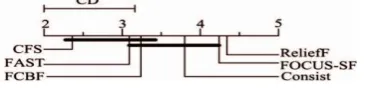
Fig. 3: Proportion of selected features comparison of all feature selection algorithms against each other with the Nemenyi test.

In order to further explore feature selection algorithms whose reduction rates have statistically significant dif-ferences, we performed a Nemenyi test. Fig. 3 shows the results with = 0.1 on the 35 data sets. The results indicate that the proportion of selected features of FAST is statistically smaller than those of RelieF, CFS and FCBF, and there is no consistent evidence to indicate sta-tistical differences between FAST , Consist, and FOCUS-SF, respectively.

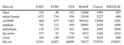
4.4.2 Runtime

TABLE 3: Runtime (in ms) of the six feature selection algorithms

Data set FAST FCBF CFS ReliefF Consist FOCUS-SF

chess 105 60 352 12660 1999 653

mfeat-fourier 1472 716 938 13918 3227 660

coil2000 866 875 1483 304162 53850 1281

elephant 783 312 905 20991 2439 1098

arrhythmia 110 115 821 3684 3492 2940

fqs-nowe 977 97 736 1072 1360 1032

colon 166 148 12249 744 1624 960

fbis.wc 14761 16207 66058 79527 579376 479651

AR10P 706 458 57319 3874 3568 2083

PIE10P 678 1223 77579 7636 4149 2910

oh0.wc 5283 5990 59624 4898 488261 420116 oh10.wc 5549 6033 28438 5652 428459 402853

B-cell1 160 248 103871 1162 2476 1310

B-cell2 626 1618 930465 4334 5102 2556

B-cell3 635 2168 1097122 7001 4666 2348

base-hock 8059 21793 146454 728900 999232 1017412 TOX-171 1750 1558 1341345 9757 17185 8446 tr12.wc 3089 3585 51360 2558 53304 34270 tr23.wc 4266 2506 32647 1585 29165 16649 tr11.wc 5086 5575 136063 4418 111073 79000 embryonal-tumours 754 314 10154 1681 5045 1273

leukemia1 449 278 10900 790 5708 1263

leukemia2 1141 456 216888 894 10407 3471 tr21.wc 4662 5543 218436 4572 89761 55644 wap.wc 25146 28724 768642 33873 1362376 1093222 PIX10P 2957 9056 25372209 11231 9875 4292 ORL10P 2330 12991 30383928 11547 13905 5780 CLL-SUB-111 1687 1870 6327479 12720 17554 12307 ohscal.wc 353283 391761 981868 655400 NA NA la2s.wc 70776 99019 2299244 118624 7400287 NA la1s.wc 79623 107110 2668871 128452 7830978 NA

GCM 9351 4939 3780146 32950 39383 26644

SMK-CAN-187 4307 5114 NA 34881 67364 38606

new3s.wc 790690 960738 NA 2228746 NA NA

GLA-BRA-180 29854 17348 NA 97641 220734 152536 Average(Image) 1520 4090 9315452 8213 6014 2793 Average(Microarry) 1468 1169 1152695 8059 9590 5385 Average(Text) 6989 8808 137232 107528 381532 327341 Average 3573 4671 2456366 45820 149932 126970 Win/Draw/Loss - 22/0/13 33/0/2 29/0/6 35/0/0 34/0/1

(11)

1) Generally the individual evaluation based feature selection algorithms of FAST, FCBF and ReliefF are much faster than the subset evaluation based algorithms of CFS, Consist and FOCUS-SF. FAST is consistently faster than all other algorithms. The runtime of FAST is only 0.1% of that of CFS, 2.4% of that of Consist, 2.8% of that of FOCUS-SF, 7.8% of that of ReliefF, and

76.5% of that of FCBF, respectively. The

Win/Draw/Loss records show that FAST outperforms other algorithms as well.

2) For image data, FAST obtains the rank of 1. Its runtime is

only 0.02% of that of CFS, 18.50% of that of ReliefF, 25.27% of that of Consist, 37.16% of that of FCBF, and 54.42% of that of FOCUS-SF, respectively. This reveals that FAST is more efficient than others when choosing features for image data.

3) For microarray data, FAST ranks 2. Its runtime is only

0.12% of that of CFS, 15.30% of that of Consist, 18.21% of that of ReliefF, 27.25% of that of FOCUS-SF, and 125.59% of that of FCBF, respectively.

4) For text data, FAST ranks 1. Its runtime is 1.83% of

that of Consist, 2.13% of that of FOCUS-SF, 5.09% of that of CFS, 6.50% of that of ReliefF, and 79.34% of that of FCBF, respectively. This indicates that FAST is more efficient than others when choosing features for text data as well.

Fig. 4: Runtime comparison of all feature selection algo-rithms against each other with the Nemenyi test.

In order to further explore whether the runtime of the six feature selection algorithms are significantly different we performed a Friedman test. The null hypothesis of the Friedman test is that all the feature selection algo-rithms are

equivalent in terms of runtime. The test result is p = 0. This

means that at = 0.1, there is evidence to reject the null hypothesis and all the six feature selection algorithms are different in terms of runtime. Thus a post-hoc Nemenyi test was conducted. Fig. 4 shows the results with = 0.1 on the 35 data sets. The results indicate that the runtime of FAST is statistically better than those of ReliefF, FOCUS-SF, CFS, and Consist, and there is no consistent evidence to indicate statistical runtime differences between FAST and FCBF.

4.4.3 Classification accuracy

Tables 4, 5, 6 and 7 show the 10-fold cross-validation

accuracies of the four different types of classifiers on the 35 data sets before and after each feature selection algorithm is performed, respectively.

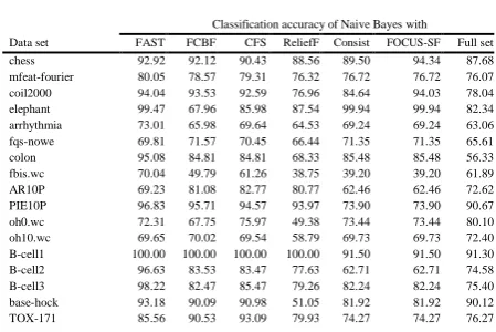
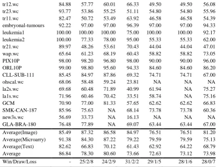
Table 4 shows the classification accuracy of Naive Bayes. From it we observe that

1) Compared with original data, the classification accuracy of Naive Bayes has been improved by FAST, CFS, and FCBF by 12.86%, 6.62%, and 4.32%,

respectively. Unfortunately, ReliefF, Consist, and FOCUS-SF have decreased the classification accu-racy by 0.32%, 1.35%, and 0.86%, respectively. FAST ranks 1 with a margin of 6.24% to the second best accuracy 80.60% of CFS. At the same time, the Win/Draw/Loss records show that FAST outper-forms all other five algorithms.

2) For image data, the classification accuracy of Naive

Bayes has been improved by FCBF, CFS, FAST, and ReliefF by 6.13%, 5.39%, 4.29%, and 3.78%, re-spectively. However, Consist and FOCUS-SF have decreased the classification accuracy by 4.69% and 4.69%, respectively. This time FAST ranks 3 with a margin of 1.83% to the best accuracy 87.32% of FCBF.

3) For microarray data, the classification accuracy of

Naive Bayes has been improved by all the six algorithms FAST, CFS, FCBF, ReliefF, Consist, and FOCUS-SF by 16.24%, 12.09%, 9.16%, 4.08%, 4.45%, and 4.45%, respectively. FAST ranks 1 with a mar-gin of 4.16% to the second best accuracy 87.22% of CFS. This indicates that FAST is more effective than others when using Naive Bayes to classify microarray data.

4) For text data, FAST and CFS have improved the classification accuracy of Naive Bayes by 13.83% and 1.33%, respectively. Other four algorithms Re-liefF, Consist, FOCUS-SF, and FCBF have decreased the accuracy by 7.36%, 5.87%, 4.57%, and 1.96%, respectively. FAST ranks 1 with a margin of 12.50% to the second best accuracy 70.12% of CFS.

TABLE 4: Accuracy of Naive Bayes with the six feature selection algorithms

(12)

tr12.wc 84.88 57.77 60.01 66.33 49.50 49.50 56.08 tr23.wc 93.77 53.86 55.25 51.11 54.80 54.80 55.96 tr11.wc 82.47 50.72 53.49 63.92 46.58 46.58 54.39 embryonal-tumours 92.22 97.00 97.00 96.39 97.00 97.00 94.33 leukemia1 100.00 100.00 100.00 75.00 100.00 100.00 92.17 leukemia2 100.00 77.33 78.00 95.00 55.33 55.33 62.00 tr21.wc 89.97 48.26 53.61 70.43 44.04 44.04 47.01 wap.wc 65.64 61.23 68.19 60.43 58.82 58.82 73.05 PIX10P 98.00 98.20 96.80 98.00 90.00 90.00 96.00 ORL10P 99.00 98.80 95.60 94.33 84.60 84.60 86.20 CLL-SUB-111 85.45 84.97 87.86 69.32 74.71 74.71 67.00

ohscal.wc 68.06 58.48 59.24 23.81 NA NA NA

la2s.wc 69.68 60.48 71.89 40.99 61.94 NA 75.27 la1s.wc 71.96 60.46 70.42 33.51 58.74 NA 75.16 GCM 70.90 77.00 81.33 57.65 62.62 62.62 66.83 SMK-CAN-187 85.96 75.63 NA 68.14 73.78 73.78 60.36

new3s.wc 56.69 33.73 NA 16.13 NA NA NA

GLA-BRA-180 76.48 77.89 NA 69.07 63.44 63.44 67.00 Average(Image) 85.49 87.32 86.58 84.97 76.51 76.51 81.20 Average(Microarry) 91.38 84.30 87.22 79.22 79.59 79.59 75.13 Average(Text) 82.62 66.83 70.12 61.43 62.92 64.22 68.79 Average 86.84 78.30 80.60 73.66 72.63 73.12 73.98 Win/Draw/Loss - 25/2/8 24/2/9 31/2/2 29/1/5 28/1/6 28/0/7

.

TABLE 5: Accuracy of C4.5 with the six feature selection algorithms

Classification accuracy of C4.5 with

Data set FAST FCBF CFS ReliefF Consist FOCUS-SF Full set chess 94.02 94.02 90.43 97.83 99.44 94.34 99.44 mfeat-fourier 71.25 75.74 77.80 76.40 71.06 71.06 75.93 coil2000 94.03 94.03 94.03 94.03 93.97 94.03 93.93 elephant 99.90 99.94 99.94 99.90 99.94 99.94 95.27 arrhythmia 71.53 70.05 69.21 66.15 66.59 66.59 65.23 fqs-nowe 69.81 73.35 69.13 66.46 68.42 68.42 66.96 colon 90.40 90.76 89.14 82.38 86.90 86.90 82.33 fbis.wc 69.41 69.35 77.52 57.03 68.70 68.70 NA AR10P 77.69 75.54 79.54 71.54 64.92 64.92 70.92 PIE10P 84.13 82.95 86.10 80.32 81.33 81.33 79.14 oh0.wc 71.88 75.45 84.20 57.43 83.47 83.47 81.37 oh10.wc 69.33 73.75 74.65 67.65 75.60 75.60 72.38 B-cell1 87.33 81.80 82.90 78.17 88.60 88.60 74.90 B-cell2 71.00 63.24 64.07 65.85 60.80 60.80 64.31 B-cell3 78.07 81.07 77.02 83.04 72.84 72.84 77.96 base-hock 92.02 89.81 89.57 49.92 90.57 90.57 91.54 TOX-171 76.85 64.92 68.69 60.24 68.66 68.66 58.44 tr12.wc 81.68 85.43 31.96 74.02 43.76 84.47 81.19 tr23.wc 89.87 94.80 46.38 86.78 67.07 96.57 92.93 tr11.wc 80.22 82.04 36.95 69.25 46.81 84.11 79.09 embryonal-tumours 87.78 97.00 97.00 88.89 97.00 97.00 87.50 leukemia1 100.00 97.00 97.00 61.11 97.00 97.00 89.17 leukemia2 100.00 75.00 78.00 88.89 81.33 81.33 60.33 tr21.wc 90.47 88.32 69.23 80.26 68.76 88.21 80.72 wap.wc 62.26 67.60 32.87 64.32 21.86 63.27 NA PIX10P 97.00 95.40 98.80 93.33 92.20 92.20 93.00 ORL10P 90.33 82.60 90.20 74.67 84.00 84.00 72.40 CLL-SUB-111 83.64 73.85 74.36 64.80 78.76 78.76 60.89

ohscal.wc 67.73 66.69 68.42 27.30 NA NA NA

la2s.wc 72.40 72.53 79.08 51.52 75.53 NA NA

la1s.wc 72.45 72.57 77.63 47.05 75.33 NA NA

GCM 58.73 59.16 60.92 52.73 45.79 45.79 51.81 SMK-CAN-187 85.19 71.42 NA 66.14 77.83 77.83 62.17

new3s.wc 55.64 60.51 NA 17.83 NA NA NA

Table 5 shows the classification accuracy of C4.5. From it we observe that

1) Compared with original data, the classification accuracy of

C4.5 has been improved by FAST, FCBF, and FOCUS-SF by 4.69%, 3.43%, and 2.58%, respectively. Unfortunately,

ReliefF, Consist, and CFS have decreased the

classification accuracy by 3.49%, 3.05%, and 2.31%, respectively. FAST obtains the rank of 1 with a margin of 1.26% to the second best accuracy 81.17% of FCBF.

2) For image data, the classification accuracy of C4.5 has

been improved by all the six feature selection algorithms FAST, FCBF, CFS, ReliefF, Consist, and FOCUS-SF by 5.31%, 4.54%, 7.20%, 0.73%, 0.60%, and 0.60%, respectively. This time FAST ranks 2 with a margin of 1.89% to the best accuracy 83.6% of CFS and a margin of 4.71% to the worst accuracy 76.99% of Consist and FOCUS-SF.

3) For microarray data, the classification accuracy of C4.5

(13)

For text data, the classification accuracy of C4.5 has been decreased by algorithms FAST, FCBF, CFS, ReliefF, Consist and FOCUS-SF by 4.46%, 2.70%, 19.68%, 13.25%, 16.75%, and

1.90% respectively. FAST ranks 3 with a margin of 2.56% to the best accuracy 83.94% of FOCUS-SF and a margin of 15.22% to

the worst accuracy 66.16% of CFS.

TABLE 6: Accuracy of IB1 with the six feature selection algorithms

Classification accuracy of IB1 with

Data set FAST FCBF CFS ReliefF Consist FOCUS-SF Full set chess 90.18 91.47 84.78 96.86 95.09 90.79 90.60 mfeat-fourier 77.87 81.69 83.72 80.00 77.71 77.71 80.13 coil2000 88.42 89.27 89.42 89.16 89.96 67.62 89.87 elephant 98.97 99.99 99.99 100.00 99.97 99.97 99.31 arrhythmia 64.48 60.10 63.67 54.35 55.22 55.22 53.27 fqs-nowe 56.59 66.20 70.48 70.74 63.02 63.02 65.32 colon 91.90 78.76 84.38 82.54 85.95 85.95 76.14 fbis.wc 60.09 61.91 72.94 43.69 60.83 60.83 NA AR10P 73.33 79.08 86.77 71.79 80.46 80.46 49.54 PIE10P 99.21 99.90 99.05 99.37 92.19 92.19 99.62 oh0.wc 67.33 63.19 75.53 48.12 68.34 68.34 20.64 oh10.wc 64.06 63.56 66.46 56.67 63.41 63.41 8.40 B-cell1 100.00 94.90 95.40 92.17 93.30 93.30 73.00 B-cell2 97.00 87.02 86.42 71.78 58.00 58.00 70.20 B-cell3 98.96 95.02 95.02 83.48 80.20 80.20 83.98 base-hock 89.06 92.24 92.60 50.86 92.95 92.95 78.81 TOX-171 75.60 95.92 97.90 96.32 65.14 65.14 86.44 tr12.wc 82.11 83.43 84.92 61.02 84.91 84.91 40.13 tr23.wc 90.18 86.55 88.90 67.62 86.80 86.80 56.11 tr11.wc 78.43 79.65 81.89 59.81 81.26 81.26 49.58 embryonal-tumours 90.56 97.00 97.00 90.56 97.00 97.00 89.50 leukemia1 100.00 97.00 97.00 67.22 97.00 97.00 76.50 leukemia2 100.00 84.33 75.00 79.72 71.00 71.00 59.67 tr21.wc 87.98 85.34 91.23 76.41 87.23 87.23 67.85 wap.wc 56.47 57.31 68.49 61.03 58.74 58.74 NA PIX10P 99.00 99.00 99.00 99.00 95.00 95.00 99.00 ORL10P 100.00 97.60 95.20 94.67 95.00 95.00 94.40 CLL-SUB-111 79.09 74.94 81.62 68.66 65.83 65.83 NA

ohscal.wc 52.94 49.52 57.98 19.67 NA NA NA

la2s.wc 68.33 68.16 79.88 39.95 73.43 NA NA

la1s.wc 67.44 67.01 76.41 33.98 71.42 NA NA

GCM 68.49 66.71 69.50 58.59 52.54 52.54 58.87 SMK-CAN-187 76.28 66.08 NA 70.40 70.58 70.58 63.57

new3s.wc 49.46 52.38 NA 8.82 NA NA NA

Table 6 shows the classification accuracy of IB1. From it we observe that

1) Compared with original data, the classification ac-curacy

of IB1 has been improved by all the six fea-ture selection algorithms FAST, FCBF, CFS, ReliefF, Consist, and FOCUS-SF by 13.75%, 13.19%, 15.44%, 5.02%, 9.23%, and 8.31%, respectively. FAST ranks 2 with a margin of 1.69% to the best accuracy 85.32% of CFS. The Win/Draw/Loss records show that FAST outperforms all other algorithms except for CFS, winning and losing on 14 and 20 out of the 35 data sets, respectively.

Although FAST does not perform better than CFS, we observe that CFS is not available on the three biggest data sets of the 35 data sets. Moreover, CFS is very slow compared with other algorithms as reported in Section 4.4.2.

2) For image data, the classification accuracy of IB1 has been

improved by all the six feature selection algorithms FAST, FCBF, CFS, ReliefF, Consist, and FOCUS-SF by 3.00%, 5.91%, 7.70%, 4.59%, 2.56%, and 2.56%, respectively.

FAST ranks 4 with a mar-gin of 4.70% to the best accuracy 89.04% of CFS.

3)

For microarray data, the classification accuracy of IB1

has been improved by all the six algorithms FAST, FCBF, CFS, ReliefF, Consist, and FOCUS-SF by 13.58%, 10.80%, 11.74%, 3.61%, 1.59%, and 1.59%, respectively. FAST ranks 1 with a margin of 1.85% to the second best accuracy 86.91% of CFS and a margin of 11.99% to the worst accuracy 76.76% of Consist and FOCUS-SF.

4) For text data, the classification accuracy of IB1 has

been improved by the five feature selec-tion algorithms FAST, FCBF, CFS, ReliefF, Consist, and FOCUS-SF by 21.89%, 21.85%, 25.78%, 8.88%, 23.27%, and 20.85%, respectively. FAST ranks 3 with a margin of 3.90% to the best accuracy 81.56% of CFS.

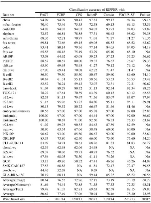
TABLE 7: Accuracy of RIPPER with the six feature selection algorithms

Data set

Classification accuracy of RIPPER with

FAST FCBF CFS ReliefF Consist FOCUS-SF Full set chess 94.09 94.09 90.43 97.81 99.17 94.34 99.16 mfeat-fourier 70.40 73.46 75.35 72.58 69.13 69.13 73.36 coil2000 94.02 94.03 94.03 94.03 93.93 94.03 93.89 elephant 72.57 66.84 78.85 77.31 98.62 98.62 79.38 arrhythmia 68.36 72.21 70.97 71.01 71.27 71.27 71.36 fqs-nowe 69.81 73.66 69.15 69.05 68.52 68.52 63.62 colon 93.41 80.14 79.76 77.14 84.05 84.05 74.19 fbis.wc 65.58 68.18 75.49 53.29 65.10 65.10 NA AR10P 73.08 64.62 65.08 59.23 57.23 57.23 56.62 PIE10P 88.57 80.57 80.00 79.37 76.67 76.67 79.33

oh0.wc 65.90 69.93 78.98 41.27 79.12 79.12 NA

oh10.wc 67.90 69.41 70.08 62.22 71.47 71.47 NA B-cell1 86.50 79.50 85.50 80.67 89.60 89.60 74.10 B-cell2 80.67 61.31 55.13 58.56 53.53 53.53 53.42 B-cell3 82.52 76.24 59.42 72.07 72.31 72.31 60.67 base-hock 91.04 89.29 90.72 51.13 92.34 92.34 88.26 TOX-171 78.22 67.61 70.59 63.39 60.12 60.12 62.58 tr12.wc 82.53 81.13 79.67 71.56 83.07 83.07 77.94 tr23.wc 91.15 95.96 93.22 84.80 95.11 95.11 89.91 tr11.wc 80.13 79.52 80.72 66.67 81.46 81.46 NA embryonal-tumours 80.56 97.00 97.00 85.28 97.00 97.00 82.83 leukemia1 100.00 97.00 97.00 64.44 97.00 97.00 86.67 leukemia2 100.00 70.67 71.00 92.50 76.33 76.33 63.67 tr21.wc 91.07 89.75 90.53 84.63 87.59 87.59 NA

wap.wc 50.90 63.54 67.06 58.48 60.00 60.00 NA

PIX10P 96.67 93.00 85.80 86.67 92.00 92.00 82.60 ORL10P 85.33 73.80 62.40 66.00 75.60 75.60 54.20 CLL-SUB-111 83.99 74.91 70.61 68.76 81.83 81.83 66.77

ohscal.wc 62.34 62.98 62.06 24.98 NA NA NA

la2s.wc 69.37 70.06 79.73 40.93 76.52 NA NA

la1s.wc 67.56 68.03 78.50 41.11 74.26 NA NA

GCM 53.13 49.86 50.32 47.41 46.26 46.26 44.09

SMK-CAN-187 77.53 68.88 NA 61.81 72.47 72.47 59.55

new3s.wc 44.46 52.69 NA 9.69 NA NA NA

Table 7 shows the classification accuracy of RIPPER. From it we observe that

1) Compared with original data, the classification ac-curacy

(14)

78.46% of Consist. The Win/Draw/Loss records show that FAST outperforms all other algorithms.

2) For image data, the classification accuracy of RIP-PER has

been improved by all the six feature selec-tion algorithms FAST, FCBF, CFS, ReliefF, Consist, and FOCUS-SF by 12.35%, 8.23 %, 4.67%, 3.86%, 4.90%, and 4.90%, respectively. FAST ranks 1 with a

margin of 4.13% to the second best accuracy 76.52% of FCBF.

3) For microarray data, the classification accuracy of RIPPER

has been improved by all the six al-gorithms FAST, FCBF, CFS, ReliefF, Consist, and FOCUS-SF by 13.35%, 6.13%, 5.54%, 3.23%, 9.02%, and 9.02%, respectively. FAST ranks 1 with a

mar-gin of 4.33% to the second best accuracy 77.33% of Consist and FOCUS-SF.

4) For text data, the classification accuracy of RIPPER has

been decreased by FAST, FCBF, CFS, ReliefF, Consist, and FOCUS-SF by 10.35%, 8.48%, 7.02%, 20.21%, 7.25%, and 7.68%, respectively. FAST ranks 5 with a margin of 3.33% to the best accuracy 82.81% of CFS.

In order to further explore whether the classification accuracies of each classifier with the six feature selection algorithms are significantly different, we performed four Friedman tests individually. The null hypotheses are that the accuracies are equivalent for each of the four classifiers with

the six feature selection algorithms. The test results are p = 0.

This means that at = 0.1, there are evidences to reject the null hypotheses and the accuracies are different further differences exist in the six feature selection algorithms. Thus four post-hoc Nemenyi tests were conducted. Figs. 5, 6, 7, and 8 show the results with = 0.1 on the 35 data sets.

Fig. 5: Accuracy comparison of Naive Bayes with the six feature selection algorithms against each other with the Nemenyi test.

Fig. 6: Accuracy comparison of C4.5 with the six fea-ture selection algorithms against each other with the Nemenyi test.

Fig. 7: Accuracy comparison of IB1 with the six fea-ture selection algorithms against each other with the Nemenyi test.

Fig. 8: Accuracy comparison of RIPPER with the six feature selection algorithms against each other with the Nemenyi test.

From Fig. 5 we observe that the accuracy of Naive Bayes with FAST is statistically better than those with ReliefF, Consist, and FOCUS-SF. But there is no consis-tent evidence to indicate statistical accuracy differences between Naive Bayes with FAST and with CFS, which also holds for Naive Bayes with FAST and with FCBF.

From Fig. 6 we observe that the accuracy of C4.5 with FAST is statistically better than those with ReliefF, Con-sist, and FOCUS-SF. But there is no consistent evidence to indicate statistical accuracy differences between C4.5 with FAST and with FCBF, which also holds for C4.5 with FAST and with CFS.

From Fig. 7 we observe that the accuracy of IB1 with FAST is statistically better than those with ReliefF. But there is no consistent evidence to indicate statistical accuracy differences between IB1 with FAST and with FCBF, Consist, and FOCUS-SF, respectively, which also holds for IB1 with FAST and with CFS.

From Fig. 8 we observe that the accuracy of RIPPER with FAST is statistically better than those with ReliefF. But there is no consistent evidence to indicate statistical accuracy differences between RIPPER with FAST and with FCBF, CFS, Consist, and FOCUS-SF, respectively.

For the purpose of exploring the relationship between feature selection algorithms and data types, i.e. which algorithms are more suitable for which types of data, we rank the six feature selection algorithms according to the classification accuracy of a given classifier on a specific type of data after the feature selection algorithms are performed. Then we summarize the ranks of the feature selection algorithms under the four different clas-sifiers, and give the final ranks of the feature selection algorithms on different types of data. Table 8 shows the results.

(15)

for all data, FAST ranks 1 and should be the undisputed first choice, and FCBF, CFS are good alternatives.

From the analysis above we can know that FAST performs very well on the microarray data. The reason lies in both the characteristics of the data set itself and the property of the proposed algorithm.

Microarray data has the nature of the large number of features (genes) but small sample size, which can cause “curse of dimensionality” and over-fitting of the training data [19]. In the presence of hundreds or thousands of

features, researchers notice that it is common that a large number of features are not informative because they are either irrelevant or redundant with respect to the class concept [66]. Therefore, selecting a small number of discriminative genes from thousands of genes is essential for successful sample classification [27], [66].

Our proposed FAST effectively filters out a mass of irrelevant features in the first step. This reduces the possibility of improperly bringing the irrelevant features into the subsequent analysis. Then, in the second step, FAST removes a large number of redundant features by choosing a single representative feature from each cluster of redundant features. As a result, only a very small number of discriminative features are selected. This coincides with the desire happens of the microarray data analysis.

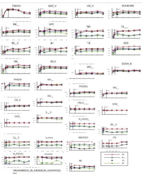
4.4.4 Sensitivity analysis

Like many other feature selection algorithms, our pro-posed FAST also requires a par