A Study of the Use of Process Simulation and Pilot-Scale Verification Trials for the Design of Bioprocesses
by
Andrew Irvin CLARKSON
Thesis submitted for the degree of Doctor of Philosophy
in
The Advanced Centre for Biochemical Engineering D epartm ent of Chemical and Biochemical Engineering
University College London T orrington Place
London W C IE 7JE
ProQ uest Number: 10017237
All rights reserved
INFORMATION TO ALL U SE R S
The quality of this reproduction is d ep en d en t upon the quality of the copy subm itted.
In the unlikely even t that the author did not sen d a com plete manuscript
and there are m issing p a g e s, th e se will be noted. Also, if material had to be rem oved, a note will indicate the deletion.
uest.
ProQ uest 10017237
Published by ProQ uest LLC(2016). Copyright of the Dissertation is held by the Author.
All rights reserved.
This work is protected against unauthorized copying under Title 17, United S ta tes C ode. Microform Edition © ProQ uest LLC.
ProQ uest LLC
789 East E isenhow er Parkway P.O. Box 1346
ACKNOWLEDGMENTS
I would like to thank the following individuals who have all helped and encouraged me in producing this thesis. First of all my project supervisor, Dr. Nigel Titchener- Hooker for his guidance, support and endless editing. My project advisor. Prof. Peter Dunnill for providing me with the benefit of his experience and Dr. David Bogle for his help and advice on the use of SpeedUp.
All experimental work and analysis was conducted with Dr. Mark Bulmer without whose help a large proportion of this work would not have been possible. I would like to thank Mr. Billy Doyle for his help and advice in all matters relating to the pilot- plant, and the workshop staff for their quick repairs when needed. I would also like to thank the other members of the Simulation and Design Group ; namely Somaiya Siddiqi and Gerardo Aquilera-Soriano for the numerous helpful discussions.
ABSTRACT
This thesis examines the use of process simulation tools and pilot-scale verification trials for the design of efficient bioprocesses. The use of process simulation tools requires the development of predictive, robust unit operation models were the models are used for the calculation of mass and energy balances, and ultimately economic analysis and optimisation. Verification trials are employed to assess how the model compares to reality. Models describing key unit operations such as protein precipitation and centrifugation are often very simplistic and do not take into account the added complications that biological materials present, such as hindered settling at high solids concentrations in centrifuges and susceptibility to shear forces. The generation of useful engineering models, testing by comparison with real process data and their use in design are covered in this work.
Two models have been developed in this thesis; batch protein precipitation and disc- stack centrifugation. The batch protein precipitation model calculates the enzyme and total protein solubilities upon precipitant addition, together with the precipitate phase particle size distribution and enables the effects of precipitant concentration and batch ageing conditions to be predicted. A mass and activity balance is then completed around the unit operation. The disc-stack centrifuge model is capable of predicting the separation of a range of biological materials including whole yeast cell, cell debris and shear-sensitive precipitate particle suspensions. A centrifuge feedzone breakage model has also been developed, which accounts for the shear breakage of
precipitate particle suspensions that occurs in the feedzone of the centrifuge. The capacity to predict the much finer particle size distribution which enters the active
disc stack where particle separation occurs enables accurate predictions of separation perform ance to be made. The centrifuge model also enables mass and activity balances to be completed around the unit operation.
The models developed for the yeast ADH test bed have also been tested for a process for the isolation of p-galactosidase from Escherichia coli. Results have shown that only limited experimental data is required to calculate the parameters used in the models to effect an accurate simulation.
Table of Contents
A C KN OW LED GM EN TS
ABSTRACT
IN TR O D U C TIO N .... 18
1.1 Design of Downstream Processes ....18
1.1.1 C urrent Practice .... 18
1.1.2 C om puter-A ided Design of Downstream Processes .... 19
1.1.3 Process Synthesis .... 19
1.1.4 Process Simulation ....22
1.1.5 Model Development ....25
1.1.6 Bioprocess Simulation ....25
1.1.6.1 Development of a Bioprocess Simulator ....27 1.1.6.2 Bioprocesses and Simulation ....28
1.1.7 Conclusions ....30
1.2 Modelling of Protein Precipitation .... 31
1.2.1 Solubility Considerations .... 31
1.2.2 Fractional Precipitation ....36
1.2.2.1 Empirical Fractionation Cuts .... 36 1.2.2.2 Specific Property Solubility Test ....36 1.2.2.3 Derivative Solubility Line M ethod ....37
1.2.2.4 Fractionation Diagrams ....38
1.2.3 Particle Size Distribution Considerations ....42 1.2.3.1 Protein Precipitate Aggregate Growth ....42 1.2.3.2 Protein Precipitate Aggregate Breakage ....45
1.2.3.3 The Population Balance .... 47
1.2.4 Ageing of Precipitates ....52
1.2.4.1 Batch Ageing ....52
1.2.4.2 Continuous Ageing ....53
1.2.5 Conclusions ....55
1.3 Modelling of Centrifugation ....56
1.3.1 Theory of Centrifugal Sedimentation .... 56
1.3.1.1 The Sigma Concept .... 57
1.3.1.2 The Grade Efficiency Concept ....59 1.3.2 Centrifuge Fluid and Particle Dynamics .... 61 1.3.3 Centrifugal Recovery of Biological Particles ....62
1.3.3.2 Shear Disruption of Biological Floes .... 64
1.3.4 Conclusions .... 65
1.4 Aims of Research ....66
M A TERIA LS AND M ETHODS ....67
2.1 Introduction ....67
2.2 Choice of Experim ental System ....67
2.3 Assay, Analysis, Reagents and Methods ....68
2.3.1 Total Protein Concentration ....68
2.3.1.1 Bradford Assay . ..69
2.3.1.2 Bicinchoninic Acid Assay .... 69
2.3.2 Alcohol Dehydrogenase Activity ....69
2.3.3 DNA Concentration ....70
2.3.4 Cell Debris Concentration .... 70
2.3.5 Dry and Wet Weights ....71
2.3.6 Packed Weights ....71
2.3.7 Particle Size Analysis ....71
2.3.7.1 Electrical Sensing Zone Method .... 71 2.3.7.2 Disc Photosedimentation Method .... 73
2.4 Yeast Homogenate Preparation ....75
2.4.1 Small Scale Preparation .... 75
2.4.2 Medium Scale Preparation ,...75
2.4.3 Large Scale Preparation ....76
2.5 Precipitation Studies ....76
2.6 Centrifugation Studies ....78
2.6.1 Whole Cell Suspensions ....78
2.6.2 Cell Debris Suspensions ....78
2.6.3 Protein Precipitate Suspensions ....78
2.6.4 Breakthrough Curves ....79
2.7 Verification Studies ....79
2.7.1 Small Scale Studies ....79
2.7.2 Large Scale Studies ....80
2.7.2.1 Yeast Ferm entation and Harvesting ....80
2.7.2.2 Downstream Processing ....81
2.8 Simulation Studies ....86
2.8.1 SpeedUp ....86
M O D ELLIN G OF PR OTEIN PRECIPITATION ....89
3.1 Introduction ....89
3.2 Model Development .... 89
3.2.1 Solubility Profiles ....90
3.2.2 Mass Balances ....91
3.2.3 Precipitate Particle size Distributions ....92
3.3 Parameter Estimation .... 97
3.4 Materials and Methods ....98
3.5 Results and Discussion ....99
3.6 Conclusions ....107
M O D ELLIN G OF C E N T R IF U G A T IO N ....132
4.1 Introduction ....132
4.2 Theory ..,.132
4.3 Model Development ....137
4.3.1 Particle Separation .,..138
4.3.2 H indered Settling ....138
4.3.3 Particle Breakage ....139
4.3.4 Mass Balances ....141
4.4 Parameter Estimation ....143
4.5 Materials and Methods ....146
4.5.1 Preparation of Yeast Whole Cell and
Cell Debris Suspensions ....146
4.5.2 Preparation of Precipitate Particle Suspensions ....146
4.6 Results and Discussion ....147
4.6.1 Centrifuge Breakthrough Curves ....147
4.6.2 Whole Yeast Cell and Cell Debris Suspensions ....148
4.6.3 Precipitate Particle Suspensions ....150
4.7 Conclusions ....154
PROCESS V E RIFIC A TIO N ....171
5.1 Introduction ....171
5.2 The Process Flowsheet ....171
5.3 Process Simulation ....172
5.3.1 Homogenisation Model ....172
5.3.2 Tubular Bowl Centrifuge Model ....174
5.4 Materials and Methods ....175
5.4.1 Small Scale Operation ....175
5.5 Results and Discussion ,,..176
5.5.1 Small Scale Trials ....176
5.5.2 Large Scale Trials ....179
5.5.3 Process Perturbations ....182
5.6 Conclusions ....183
6. CASE STUDY -ISO LATIO N OF p*GALACTOSIDASE FROM
E S C H E R IC H IA C O LI ....201
6.1 Introduction ....201
6.2 The Process Flowsheet ....201
6.3 Process Simulation ....201
6.3.1 Process Models ....202
6.3.1.1 Homogeniser Model ....202
6.3.1.2 Nucleic Acid Precipitation Model ....203 6.3.1.3 Protein Precipitation Model ....204
6.3.1.4 Centrifuge Model ....204
6.4 Results and Discussion ....205
6.5 Conclusions ....208
7 CONCLUSIONS ....221
8 F U T U R E WORK ....224
APPENDICES ....225
A PPEN D IX A1 D E N A T U R A T IO N STUDIES ....225
A l . l Introduction ....225
A1.2 Materials and Methods ....225
A1.3 Results and Discussion ....225
A1.4 Conclusions ....226
A P PEN D IX A2 METHODS OF PR O TEIN PRECIPITATION ....227
A2.1 Salting-out ....227
A2.2 Isoelectric Precipitation ....228
A2.3 Precipitation by Organic Solvents ....228
A2.4 Precipitation by High Molecular Weight Polymers ....228
APPEND IX A3 C E N T R IF U G E DESIGNS ....230
A3.1 The Tubular Bowl Centrifuge ....230
A3.2 The M ulticham ber Centrifuge ....230
A3.3 The Disc Stack Centrifuge ....231
A3.4 The Scroll Decanter Centrifuge ....232
A3.5 The Basket Centrifuge ....232
APPEN D IX A4 SPEEDUP MODELS ....234
A4.1 Introduction ....234
A4.2 Batch Precipitation Model ....234
A4.3 Disc Stack Centrifuge Model ....239
A4.4 Disc Stack Centrifuge Feedzone Model ....243
A PPEN D IX A5 PUBLICATIONS ....246
A5.1 Introduction ....246
A5.2 Papers ....246
N O M E N C L A T U R E ....247
List of Figures
Figure Title Page
1.1 Stages in Process Flowsheeting (Jackson and DeSilva, 1985) .... 23 1.2 The Cyclic Process of Mathematical Model Development ....26 1.3 Example of Specific Property Solubility Test for a Product Enzyme
in the Presence of M o r e - a n d Less-Soluble Protein Contaminants ....40 1.4 Example of Derivative Solubility M ethod, the Shaded Area is the
A m ount of Protein Precipitated Between Cuts C l and C2 ....40 1.5 Hypothetical Enzyme and Total Protein Solubility Profiles in the
Presence of Increasing Concentrations of Precipitant .... 41 1.6 Hypothetical E nzym e-T otal Protein Fractionation Diagram ....41 1.7 Transform ation of the Particle Size Distribution Due to Precipitate
Breakage in the Centrifuge Feedzone and Clarification ....65 2.1 Soluble and Precipitate Phase Material Assay Procedures ....68 2.2 Schematic Diagram of the Electrical Sensing Zone E quipm ent ....72 2.3 Schematic Diagram of the Disc Photosedimentometer Equipm ent ....74 2.4 Schematic Diagram of the Precipitation Reactors of 1.4 L, 4.4 L and
120 L Scales .... 77
2.5 Block Flow Diagram of the Resuspended Bakers Yeast Process ....82 2.6 Block Flow Diagram of the Ferm ented Yeast Process ....83
2.7 Schematic Diagram of SpeedUp Architecture ....87
3.1 Flowchart for the Protein Precipitate Param eter Estimation
Routines ....108
3.2 Fraction Remaining Soluble Plotted Against Precipitant Concentration, as a Function of the Constants a and m in
equation (3.1) ....109
3.3 Fraction Rem aining Soluble Plotted Against Precipitant Concentration, as a Function of the Constants a and m in
equation (3.1) . ..110
3.4 Normalised Log-N orm al distribution Constructed with a Geometric Mean Size, d ^ of 1.5 pm and a Geometric Standard
Deviation, o of 1.5 pm ... 111
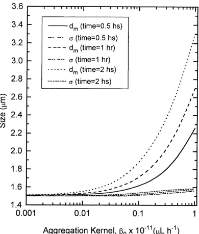
3.5 Geometric Mean size, d ^ and Geometric Standard Deviation, o Plotted Against the Aggregation Kernal, Pq a Function
of the Batch Ageing Time ...112
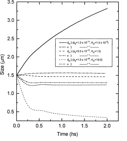
3.6 Geometric Mean size, d ^ and Geometric Standard Deviation,
Function of the Batch Ageing Time ....113 3.7 Geometric Mean size, and Geometric Standard Deviation,
a Plotted Against Batch Ageing Time as a Function of the
Aggregation Kernel, (Jg and Breakage Rate Constant, Kj^ ....114 3.8 Soluble and Precipitate Phase Total Protein Concentration
Plotted Against Ammonium Sulphate Concentration (% sat.)
for the 1.4 L Reactor ....115
3.9 Soluble and Precipitate Phase AD H Activity Plotted Against Ammonium Sulphate Concentration (% sat.) for
the 1.4 L Reactor ....116
3.10 Precipitate Phase Total Protein Concentration Plotted Against Batch Ageing Time as a Function of Ammonium
Sulphate Concentration (% sat.) ....117
3.11 Precipitate Phase AD H Activity Plotted Against Batch Ageing
Time as a Function of A m m onium Sulphate Concentration (% sat.) ....118 3.12 Total Protein and AD H Fraction Soluble Plotted
Against A m m onium Sulphate Concentration (% sat.) for
the 1.4 L Reactor ....119
3.13 Total Protein Fraction Soluble Derived From Equation (3.1) Plotted Against A m m onium Sulphate Concentration (% sat.) for the 1.4 L, 4.4 L and 120 L Precipitation
Reactors ....120
3.14 A D H Fraction Soluble Derived From Equation (3.1)
Plotted Against Am m onium Sulphate Concentration (% sat.)
for the 1.4 L, 4.4 L and 120 L Precipitation Reactors ....121 3.15 Average Total Protein and AD H Fraction Soluble Derived
From Equation (3.1) Plotted Against A m m onium Sulphate
Concentration (% sat.) ....122
3.16 Total Protein and AD H Constant a From Equation (3.1) for the Second Cut Precipitation Plotted Against the Position of the First Cut Precipitation in A m m onium Sulphate
Concentration (% sat.) ....123
3.17 Total Protein and AD H Constant m From Equation (3.1) for the Second Cut Precipitation Plotted Against the Position of the First Cut Precipitation in Am m onium Sulphate
Concentration (% sat.) ....124
3.18 Normalised N um ber-D ensity Particle Size Distributions for 40 % sat. Material Prepared in the 1.4 L Precipitation
3.19 Variation of the Aggregation Kernel, Pq with Average Shear
Rate Within the Precipitation Reactor ....126
3.20 Variation of the Breakage Rate Constant, with Average
Shear Rate Within the Precipitation Reactor ,...127
3.21 Experimental and Simulated Normalised N um ber-D ensity Particle Size Distributions for the 1.4 L Precipitation
Reactor and Gt k 10^ ....128
3.22 Experimental and Simulated Precipitate Growth Shown by Plots of the Geometric Mean, d ^ , and Geometric Standard
Deviation, o. Against Batch Ageing Time ....129
3.23 Protein Precipitate Aggregate Density Plotted Against Aggregate Size for 40 % sat. and 60 % sat. Prepared
Material ....130
3.24 Simulated Normalised M ass-Density Particle Size Distribution for 40 % sat. Prepared Material in the
1.4 L Precipitation Reactor ....131
4.1 Flow Through the Disc Spaces of a Disc Stack Centrifuge ....155 4.2 Structure of the Centrifuge Feedzone Breakage Model and Disc
Stack Centrifuge Model ....155
4.3 Flowchart of the F O R T R A N Program to Determine the Breakage
Rate Constant, A, in the Feedzone of a Disc Stack Centrifuge ....156 4.4 Grade Efficiency Plotted Against the Normalised Diameter as a
Function of the Constants K and n in Equation (4.24) ....157 4.5 Grade Efficiency Plotted Against the Normalised Diameter as a
Function of the Constants K and n in Equation (4.24) ....158 4.6 Grade Efficiency Plotted Against the Normalised Diameter Using
Equation (4.24) with K=0.865 and n=2.08 (Mannweiler, 1989) ....159 4.7 Protein Precipitate Suspension Breakthrough Curves for the
Disc Stack Centrifuge, SAOOH 205 ....160
4.8 Effects of Hindered Settling on the Disc Stack Centrifuge, SAOOH 205 Critical Particle Diameter, Using Equation (4.25) for Whole Yeast Cell and Fully Disrupted Cell Debris
Suspensions ...161
4.9 Disc Stack Centrifuge, SAOOH 205 Grade Efficiency Plotted
Against Normalised Diameter for Whole Yeast Cells. ,...162 4.10 Disc Stack Centrifuge, SAOOH 205 Grade Efficiency Plotted
Against Normalised Diameter for Cell Debris. ....163 4.11 Simulated and Experim ental Unsedimented Solids at D ifferent
Scaled-Down to 25 % of its Separation area ..,,164 4.12 Effects of Aggregate Size-Density Function for 40 % sat.
Prepared Material in the Disc Stack Centrifuge, SAOOH 205,
Critical Particle Diameter Calculated Using Equation (3.33) ....165 4.13 Disc Stack Centrifuge SAOOH 205 Grade Efficiency Plotted
Against Normalised Diameter for a 40 % sat. Prepared
Precipitate Suspension ....166
4.14 Disc Stack Centrifuge SAOOH 205 Grade Efficiency Plotted Against Normalised Diameter for a 60 % sat. Prepared
Precipitate Suspension ....167
4.15 Disc Stack Centrifuge SAOOH 205 Feedzone Breakage Constant, A, Plotted Against Feed Flowrate for 40 % sat. and 60 %
sat. Prepared Precipitate Suspensions ....168
4.16 Percentage Unsedim ented Solids Plotted Against Feed Flowrate for a 40 % sat. Prepared Precipitate Suspensions
in the Disc Stack Centrifuge, SAOOH 205 ....169
4.17 Percentage Unsedim ented Solids Plotted Against Feed Flowrate for a 60 % sat. Prepared Precipitate Suspension
in the Disc Stack Centrifuge, SAOOH 205 ....170
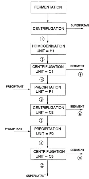
5.1 Process Flowsheet for the Recovery and Purification of
Alcohol Dehydrogenase (ADH) From Saccharomyces cerevisiae ....185 5.2 Soluble and Solid Phase Total Protein Release Plotted Against
the N um ber of Passes in the K3 Pilot-Scale Homogeniser ....186 5.3 Soluble and Solid Phase A D H Release Plotted Against the
N um ber of Passes in the K3 Pilot-Scale Homogeniser ....187 5.4 Soluble Phase Total Protein Release Plotted Against Soluble
Phase A D H Release ....188
5.5 Process Flowsheet and Experim ental Mass and Activity Balance
at a Small Scale of 3 L ....189
5.6 Experim ental and Simulated Soluble Phase Total Protein
Concentration Plotted Against Stream N um ber for the Complete
Process at a Small Scale of 3 L ....190
5.7 Experim ental and Simulated Soluble Phase Total Protein Plotted Against Stream N um ber for the Complete Process at a Small Scale
of 3 L ....191
5.8 Experim ental and Simulated Soluble Phase ADH Plotted Against Stream N um ber for the Complete Process at a Small Scale
5.9 Experim ental and Simulated Solid/Precipitate Phase Total Protein Plotted Against Stream Num ber for the Complete
Process at a Small Scale of 3 L ....193
5.10 Experim ental and Simulated Soluble Phase DNA Plotted Against Stream Num ber for the Complete Process at a Small
Scale of 3 L ....194
5.11 Experim ental and Simulated Cell Debris Plotted Against Stream N um ber for the Complete Process at a Small Scale
of 3 L ....195
5.12 Experim ental and simulated Soluble Phase Total Protein Concentration Plotted Against Stream Num ber for the
Complete Process at a Large Scale of 25 L ....196
5.13 Experim ental and Simulated Solid/Precipitate Phase ADH Plotted Against Stream Num ber for the Complete Process
at a Large Scale of 25 L ....197
5.14 Experim ental and Simulated Soluble Phase ADH Specific Activity Plotted Against Stream Num ber for the Complete
Process at a Large Scale of 25 L ....198
5.15 Experim ental and Simulated Solid/Precipitate Phase ADH Specific Activity Plotted Against Stream Num ber for the
Ferm ented Yeast Process at a Large Scale of 25 L ....199 5.16 Experim ental and Simulated Solid/Precipitate Phase AD H
Specific Activity Calculated Using the Centrifuge Feedzone Breakage Model (Chapter 4) Plotted Against Stream Num ber
for the F erm ented Yeast Process at a Large Scale of 25 L ....200 6.1 Process Flowsheet for the Isolation of P-galactosidase from
E.coli ....210
6.2 Total Protein Release Plotted Against Number of Passes During
the Homogenisation Step ....211
6.3 p-galactosidase Release Plotted Against Num ber of Passes
During the Homogenisation Step ....212
6.4 E ffe c t of H eating a Clarified Disrupted E.coli Homogenate
for Total Protein, p-galactosidase and R N A ....213 6.5 Total Protein and P~galactosidase Fraction Remaining Soluble
Plotted Against Am m onium Sulphate Concentration (% sat.) ....214 6.6 Experim ental and Simulated Total Protein Concentration Plotted
Against Stream N um ber for the Complete Process Outlined
6.7 Experim ental and Simulated |3-galactosidase Activity Plotted Against Stream Num ber for the Complete Process Outlined
in Figure 6.1 ....216
6.8 Experim ental and Simulated P-galactosidase Specific Activity Plotted Against Stream Num ber for the Complete Process Outlined
in Figure 6.1 ....217
6.9 Experim ental and Simulated p-galactosidase Plotted Against
Stream N um ber for the Complete Process Outlined in Figure 6.1 ....218 6.10 Simulated RN A Concentration plotted Against Stream Num ber
for the Complete Process Outlined in Figure 6.1 ....219 6.11 Simulated Biomass Concentration Plotted Against Stream Num ber
for the Complete Process Outlined in Figure 6.1 ....220
List of Tables
Table Title Page
1.1 Growth, Birth and Death Terms Used in Population Balances
for Protein Precipitation Systems .... 49
1.2 Centrifuge S - Values ....60
2.1 Batch Reactor Dimensions .... 77
2.2 Composition of the Fermentation Medium ....84
2.3 Composition of the Feed Medium ....85
3.1 Aggregation Mechanisms ....93
3.2 Aggregation Kernels ....94
4.1 Optimum Desludge Intervals for the Disc Stack Centrifuge,
SAOOH 205 ....148
4.2 Comparison of Experim ental and Simulated Mass Yields ....150
5.1 Constants Used in the Homogenisation Model ....173
5.2 Recovery in the 6P T ubular Bowl Centrifuge (Mosquiera et al.,
1981 and Higgins et al., 1978) ....174
5.3 Small Scale Experim ental and Simulated Data ....179 5.4 Large Scale Experim ental and Simulated Data ....182
5.5 Process Perturbations ....182
6.1 Constants Used in the Homogenisation Model ....202
1. INTRODUCTION.
The uses and advantages of bioprocess simulation have been well documented on a num ber of occasions (Cooney et al., 1986; Evans and Field, 1988; Petrides et al., 1989; Gritsis and Titchener-H ooker, 1989). Simulation packages are valuable tools for helping to solve both technical and economic problems in order to meet product specifications at affordable costs and in a reasonable tim e-fram e. This is especially true in the downstream processing of biological materials where it is recognised that the recovery and purification of many proteins and enzymes represent a m ajor proportion of the total production costs. For example, the recovery costs for (Î- galactosidase from an Escherichia coli fermentation are approximately double the ferm entation costs (Datar, 1986) and are even higher for pharmaceuticals and diagnostic proteins, such as monoclonal antibodies. The use of a process simulation tool in this instance would alleviate the large time lag between the beginning of process development and product success by acceleration of the design processes. This is the central theme of this thesis.
1.1 Design of Downstream Processes.
1.1.1 C urrent Practice.
and finally gel filtration. However, this analysis is of limited value due to the reliance on small scale studies. For the design of integrated bioprocesses in which there is neither excessive over or under capacity at each stage a systematic approach to the design of downstream equipm ent is needed. This can be accomplished using com puter-aided design packages as outlined in the following section.
1.1.2 C om puter-Aided Design of Downstream Processes.
C om puter-aided design has been used for many years in the chemical processing industry, where traditionally the e ffort has mainly concentrated on creating and using mathematical models of both unit operations and processes for process simulation, cost estimation, equipm ent sizing and process optimisation. Recently c om puter-aided design techniques have been applied to the modelling of the actual design procedure itself (process synthesis), which cannot be represented by quantitative methods and data. An outline of process synthesis and the use of computer-aids follows.
1.1.3 Process Synthesis.
The process synthesis task is to decide what process units are required in order to make a desired product, and how the units should be connected together, in a process flowsheet. The process synthesis stage generates large volumes of data and frequently raises new problems, the result of which may have a profound effect on the feasibility and optimality of the process (Niida et al., 1986). Expert or intelligent knowledge based systems are ideally suited to solving such process synthesis tasks. However, since the scope of this thesis does not include the use of expert systems, only a brie f account will be given here.
E x p e rt systems are usually used to transform ill-defined unstructured problems into more tractable ones, which can then be solved by traditional means, such as flowsheeting programs. E xpert systems work on the manipulation of symbolic models, the most common being "rule based" systems. [Other systems are based on "frames", "semantic networks", and "logic" (Lien et a l.,1 9 S l).] The expert system consists of two basic components:
• the knowledge base, and, • the inference engine.
handbooks. The inference engine expresses the human expertise in the form of IF- TH EN type rules, called production rules. The user inputs the ill-defined problem and through a series of reasoning steps the problem is manipulated into a more tractable form, eventually leading to a solution. Much of the published literature in computer- aided design of bioprocesses has focused on this approach to the process synthesis task. Stephanopoulos and Townsend (1986) indicated that the use of an expert system in bioprocess synthesis could lead to the selection of the appropriate microorganism, any necessary genetic modifications, substrates and solvents etc. for the production of a particular material. They developed a computer program to help the decision process in two diffe re nt areas:
• to identify the most promising sequences of enzyme catalysed reactions for the synthesis of a desired chemical, and,
• to establish the biological feasibility of the selected production route.
Two examples were presented which showed how the use of an expert system could assist in the design of molecules and the synthesis of feasible biochemical pathways. Stephanopoulos and Stephanopoulos (1986) used an expert system for three different problems:
• the exploration of new production routes for various bioproducts, • the design of mammalian cell biofermenters, and,
• the synthesis of downstream processing sequences for the separation and purification of proteins.
downstream processing sequences. This task was approached by making use of estimates, empirical correlations and experimental heuristics to identify and develop a sequence based around the most critical step. The system consisted of a data and knowledge base and reasoning strategies. The data and knowledge base contained information about the microorganisms, proteins and process equipment, together with sets of heuristic rules, which selected appropriate unit operations, identified design procedures, determined the operating conditions and provided initial estimates of unit efficiencies. The reasoning strategies identified the most critical step by searching for a unit operation within inherent operating condition constraints. Siletti (1988) investigated the use of an expert system for the synthesis of protein recovery processes. The work focused on the developm ent of a computer program called BioSep Designer, which consists of the following components:
• a set of databases for the necessary design information, eg. proteins and process equipm ent, a methodology for selecting and configuring the process equipment. • a procedure that generates, analyses and compares design alternatives, ie,
mimics the process synthesis procedure.
• facilities that enable the biotechnologist to participate in the design process. • knowledge acquisition facilities that help the user extend the capabilities of
the system.
The design proceeded in three distinct phases:
• Solving parts of the problem for which information is available. If the required protein and its source are known, then this is usually sufficient to specify a sequence of unit operations, though this may not be optimal.
• When design decisions are to be made, these are based on the predicted effect on the entire process. This requires models that enable the prediction of perform ance of the complete process plant and that physical property data be available. U n it operations are modelled by sets of equations that relate the performance and cost of a unit to its operating conditions and the physical properties of the materials being processed.
• When there is insufficient inform ation to distinguish among the available alternatives, then all must be considered. All design alternatives are stored until such time that sufficient inform ation exists to distinguish between them.
fermentation (Siletti, 1988). In the example 200 intermediate designs were evaluated, of which 32 were found to be near the optimal, based on final productivity. Even though BioSep Designer had not undergone a formal validation, by comparing BioSep Designer with an actual manual design, the test cases studied produced recovery processes similar to those used on a commercial scale, indicating the potential of such an approach.
1.1.4 Process Simulation.
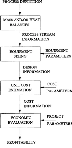
Process simulation refers to the calculation of material and energy balances for a particular process. For a large complex process manual calculation could take many months. However, process simulation can be accomplished via the flowsheeting program, (a misnomer since the flowsheet has already been developed, when such packages are used). The advantages of flowsheet simulation are many, including reducing the time taken to develop a process design, reducing the time taken to explore changes in the operating conditions, increasing productivity and process efficiency. The flowsheet simulation consists of a linked series of models where each describes in the form of mathematical equations and expressions the perform ance of each m ajor piece of equipm ent or unit operation in the process. Each unit model incorporates many physical and chemical phenomena (Evans, 1987) and in the case of bioprocess simulation, biological phenomena. The stages in process flowsheeting, as described by Jackson and Desilva (1985) are shown in Figure 1.1.
PROCESS DEFINITION
PROCESS STREAM
INFORMATION
EQUIPMENT
PARAMETERS
DESIGN
INFORMATION
COST
PARAMETERS
COST
INFORMATION
PROJECT
PARAMETERS
UNIT COST
ESTIMATION
MASS AND/OR HEAT
BALANCES
EQUIPMENT
SIZING
ECONOMIC
EVALUATION
PROFITABILITY
Three structurally different forms of flowsheeting programs exist; sequential modular, equation-oriented (simultaneous) and a combination of sequential modular and equation-oriented formats (Wells and Rose, 1986). The sequential modular system uses subroutines to calculate the output variables as functions of the input variables. That is, the sequential modular system starts at the physical beginning of the process and proceeds through the logical physical sequence of the process. For solution of the problem the process flowsheet must first be partitioned, tear streams are then selected, the convergence of the tear streams nested, and the computational sequence determined. Partitioning refers to those sets of blocks that must be solved together (defined as maximal cyclic subsystem). Tearing determines those streams and information flows that must be broken to render each subsystem acyclic. Nesting determines which tear streams are to be converged simultaneously and in which order collections of tear streams are to be converged. The basis of the equation-oriented system is to collect all of the equations describing the flowsheet and to solve them as a large system of non-linear differential and algebraic equations. Mathematically this can be stated as:
= 0 ( 1-1)
g(x,y,t)=0 (1-2)
where, x are the state or dynamic variables, y are the algebraic variables, x is the derivative of the state or dynamic variables and t is the time.
Most equations generated contain only a few variables, so that the resulting m atrix is sparse and therefore numerical solutions using methods developed for sparse matrices can significantly reduce the large computational times encountered in such problems. SPEEDUP is one such program which uses this approach (Sargent and Westerberg, 1964 and Pantelides, 1988). The main advantage of this system is the complete freedom to specify dependant and independent variables. The main disadvantages are that the equations are solved simultaneously, which can produce a meaning-less root, or no root at all. The sim ultaneous-m odular system uses two types of models; rigorous and simple. Rigorous models are used to determine parameters for the simple models, which are represented algebraically. The simple models can be solved simultaneously producing the required simulation.
accepted standards.
1.1.5 Model Development.
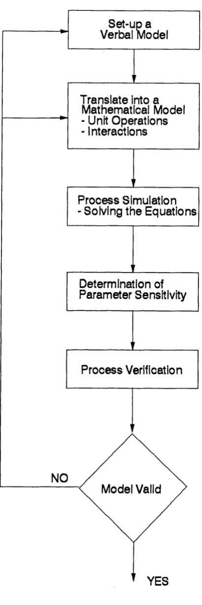
A model can be defined as a description of some real system which is intended to predict what happens when certain actions are taken. Most useful models are often simplified and idealised, and the boundaries of the system and model are rather arbitrarily defined. Model development usually starts with a written description of the problem, identifying the inputs and outputs of the model. Next a num ber of simplifying assumptions are made and rules/equations found to relate the input and output variables. Finally the model can be implemented into some computer software for ease of use. As shown in Figure 1.2. the process of model development is a cyclic one which indicates that a model is not created but developed over time with adjustments according to deviations from reality. The most significant step in the cycle is the translation of available verbal knowledge into a mathematical model. One should solve the model equations as soon as possible to get an early global impression about the perform ance of the model. If on solving the equations the results bear no resemblance to reality then the model is wrong (i.e. should be discarded) or it requires some modification to bring it closer to reality. The parameters used in the model equations influence the model result. However, the effect of parameter variation can range from very minor to very large. An early impression of the sensitivity to particular parameters provides clues to the necessary experimental s e t-u p and for the required accuracy of estimation of the parameter values. Finally model verification, in which the model predictions are compared with real data, is im portant to assess how the model compares to reality either individually or as part of an overall process.
1.1.6 BioProcess Simulation.
The use and advantages of process simulation packages in general has been documented in the previous section (1.1.4). Evans and Field (1988) have provided a review of the uses of bioprocess simulation in process development. The bioprocessing industry has yet to benefit from the widespread use of such simulation packages, but some advances have been made in their implementation. Cooney et al. (1986) outlined some of the problems encountered in bioprocess simulation, some more tractable than others:
• The unique unit operations found in a typical bioprocess are little modelled and poorly understood,
NO
M odel Valid
YES P ro c e s s Verification P ro c e s s Sim ulation - Solving th e E qu atio n s
S et-up a Verbal M odel
D eterm ination of P a ra m e ter Sensitivity T ran slate into a
M athem atical Model - Unit O perations - Interactions
• There is a high degree of process interactions between the fermentation stage and the following downstream units, and,
• The presence of batch, sem i-batch and continuous operations in a bioprocess.
A large amount of literature exists for the modelling of the initial stages of a bioprocess, such as fermentation. However, the later downstream units have been neglected, mainly due to the fact that they are less well understood (Gritsis and Titchener-H ooker, 1989). The particular procedure adopted for the modelling of downstream units depends on the level of knowledge of that particular unit. At the simplest level experimental data and curve-fitting routines can be used. At a higher level empirical models can be used with experimental data and published literature to provide values for model parameters and constants. A t the highest level models can be derived from first principles. Obviously the simplest models will lack much of the predictive capacity necessary for the generation of rigorous designs, whereas models derived from first principles should contain sufficient complexity for them to be applied in any situation but will require substantial development in the first instance.
The importance of some process interactions in bioprocesses have been documented (Fish and Lilly, 1984; Siddiqi et al., 1991; T itc he ne r-H ooke r et al., 1991). Their presence requires that an integrated approach to process design be adopted in order to evaluate the interactions between the unit operations and to ensure that a rigorous design is achieved.
1.1.6.1 Development of a Bloprocess Simulator.
Cooney et al. (1986) by adapting the simulation program ASPEN-PLUS. However, there are a num ber of problems associated with this package as outlined below:
The package is based on a sequential-m odular architecture and has limited capability of dealing with batch processes,
• The bioprocesses simulated using BPS have consisted primarily of traditional chemical engineering unit operations and hence are not well suited to describing many bioprocesses of interest.
• Physical property prediction in chemical engineering simulators will not be applicable to bioprocesses.
• The predictive capability of the software is severely limited.
A similar software package called BioDesigner is available from Intellicorp Inc. (Petrides, 1994), Although again the predictive nature of the models is somewhat limited. Gritsis and T itc he ne r-H ooke r (1989) adopted the latter approach and developed mathematical models for some common downstream unit operations using research data. The models were solved using user written F O R T R A N subroutines and the equation-based flowsheeting package, SPEEDUP. Recently, Narodoslawsky et al.,
(1993) developed a bioprocess simulator known as SIMBIOS. The program has been created to be structurally more appropriate to bioprocesses and includes mathematical models of most of the common downstream processing unit operations. What is not clear is the predictive nature of the models within the software.
1.1.6.2 Bioprocesses and Simulation.
Much of the existing work in the area of bioprocess modelling and simulation has been in the areas of ferm entation and waste treatment. In particular A htc hi-A li (1989) has used SPEEDUP for the simulation of various fermentations, and, Farag et al. (1990), has used BPS to simulate the operation of a wastewater treatm ent process. Most of the work published in the mainstream bioprocessing area has focused on the use of BPS as shown below, with only a small am ount of literature describing other methods of bioprocess simulation.
validity of the simulation results were evaluated by comparing the predicted pH of extraction with that actually used in practice. The economic feasibility of exchanging different unit operations was examined by plotting an operations curve, defining percentage efficiency plotted against a common process variable for the two operations. Cooney et al. (1986) also used BPS for the simulation of a process producing proteolytic enzymes (used in detergents). The simulation was used to size the equipm ent and to perform an economic analysis. However, no formal model validation was provided in the paper. Petrides et al. (1989) simulated the production of porcine growth hormone (pGH) from a fermentation of genetically engineered
Escherichia coli, using BPS. The input data consisted of performance characteristics for each unit operation, derived from laboratory and pilot plant experimental data. The output from the simulation gave the final product quality and quantity, as well as an economic analysis to test the feasibility of the process. Healey et al. (1990) used BPS to simulate and design a m ultiproduct processing facility, which was to produce a range of bioproducts at the lowest possible m anufacturing costs. Field (1990) provided a detailed description of the unit operation models available within ASPEN T E C H ’s BioProcess Simulator (BPS). In all of these cases little by way of experimental verification of the predictions is evident.
Using the alternative approach outlined in the previous section Gritsis and Titchener- Hooker (1989) modelled the units of ultrafiltration, precipitation and centrifugation, in a hypothetical process for the purification and recovery of an extracellular product. In the process the downstream processing equipm ent was fed from a batch ferm entation producing an extracellular product. The simulation was perform ed using s ta t e - o f - t h e - a r t numerical techniques and showed an optimal operating point for the ultrafiltration unit. The problem was then recast into an optimisation problem which was solved using Successive Quadratic Programming (SQP). However, no model validation was described or any indication how this process or simulation could be used in real situations. Siddiqi et al. (1991) identified and modelled the process interactions between a high-pressure homogeniser and the subsequent centrifugation step for the removal of cell debris, in a typical downstream process train for the recovery of an intracellular product. It was shown how properties such as viscosity and particle size affect the efficiency of the centrifugation step. Middleberg et al.
account. In a second paper based on the recovery and purification of protein inclusion bodies from £.co/t, Middleberg et al., (1992a) modelled process interactions between the combined homogenisation and centrifugation steps using SpeedUp. In the process the inclusion bodies were fractionated from the cell debris using a disc-stack centrifuge. It was identified that disruption for 2 passes released 99 % of the inclusion bodies but led to poor fractionation of the inclusion bodies from the cell debris, due to the large size of the cell debris. Homogenisation for 4 passes produced much smaller cell debris and thus improved fractionation of the inclusion bodies from the cell debris, which illustrates the importance of incorporating process interactions in the simulations. Bogle et al. (1991) used SpeedUp and Mathematica for the design and optimisation of a process producing porcine Somatotropin (pST) from a ferm entation of genetically modified Escherichia coli. The results of the modelling were also to be used to indicate areas for further research. Bogle et al. (1991) identified a num ber of process interactions between the unit operations and it was therefore necessary to consider several of the unit operations simultaneously. By matching model predictions with experimental data it was possible to postulate mechanisms for product formation. However, a num ber of assumptions were made in the modelling and the relationship between homogeniser pressure and num ber of passes with the cell debris size distribution was unquantifiable. Middleberg et al., (1992b) developed a model for the disruption of E.coli for 1 homogeniser pass and provided experimental data for model verification. The fraction of cells disrupted was provided as the product of the distribution of effective cell strengths and the distribution of stresses in the homogeniser. The effective cell strength distribution was given as a bimodal normal distribution with terms for non-septated cells and septated cells. In the model disruption was completely described by two physically m eaningful parameters for a given homogeniser ; a mean effective cell strength and a septated volume fraction of the bacterial population. It was proposed that the model accounted for process interactions between the ferm enter and homogeniser. In a second paper Middleberg
et al., (1992c) provided a correlation for the mean effective cell strength which was dependant on the cell strength and the degree of crosslinkage. In a third paper Middleberg (1993) extended the homogeniser model to include multiple passes by incorporation of one parameter, the num ber of passes, N.
1.1.7 Conclusions
interactions. Both approaches require the development of mathematical models for the unique unit operations found in a typical bioprocess. During such model development, parameter estimation routines and model verification trials need to be developed.
The following section presents a literature review of the modelling of two common downstream unit operations which will be examined further in this thesis. The review will be divided in two sections ; one covering the modelling of protein precipitation, and the other covering the modelling of centrifugation.
1.2 M odelling o f P recipitation.
Protein precipitation is one of the most im portant and widely used unit operations for the laboratory and industrial recovery, and purification of proteins. There are generally two methods for precipitating proteins. The first is where high concentrations of the precipitant are added which change the nature of the solvent environment. The second method is where a low concentration of reagent is added which interacts directly with the protein particles. The most common methods used for protein precipitation are salting-out, isoelectric precipitation and polyelectrolyte precipitation. These methods and others are reviewed in Appendix A2,
The main issues involved in the modelling of a precipitation stage are two-fold. Firstly, the model needs to be able to describe accurately the changes in solubility upon addition of the precipitant, and secondly, to describe the subsequent particle size distribution (PSD) produced. The following sections outline some of the methods used to describe the solubility and the particle size distribution of precipitating systems.
1.2.1 S olubility C onsiderations.
In the modelling of any protein precipitation process it is im portant to be able to predict the changes in protein solubility on addition of the precipitant. A small num ber of theories have been proposed ranging from fundam ental approaches to totally empirical ones. The theories tend to fall into two categories; those dealing with the salting-out of proteins and those dealing with precipitation by non-ionic polymers such as PEG.
salting-out effects. Kirkwoods model gives an approximate expression for the work expended in changing a dipolar ion in the presence of a surrounding ion atmosphere, and is valid in the limiting case of an infinitely dilute solution. This expression was then applied to the model system of a sphere with a point dipole at its centre. The dipolar ion is treated as a cavity of low dielectric constant in which the surrounding ions are distributed. Kirkwoods model can be written as:
log (1.3)
f(bi/ac)=1.96 when bj/ac=0.9 f(bi/ac)=1.00 when bi/a(-=0.0
where S is the protein solubility, Sg is the protein solubility at zero ionic strength, I is the ionic strength and is given by l/22CgZ^, Cg is the salt concentration, z is the ionic charge, p is the ionic dipole moment, Dj^ is the dielectric constant of the medium, T is the absolute tem perature, bj is the ionic radius, a(- is the collision diameter and is given by bj+(mean ionic radius), and A and B are constants for a given dipolar ion.
The expression can be separated into two parts, one proportional to p/(Dj^T)^, which is the contribution from the electrostatic interaction of the dipole and surrounding ions and corresponds to the salting-in effect, and the second, proportional to (Dj^T)'^, which is independent of the dipole moment and corresponds to the salting-out effect. The main problem with Kirkwoods expression as outlined by Puett et al. (1965) is that the salting-out term is only a minor one and this does not correlate with that found in practice. Also Kirkwoods limiting law would predict an overall salting-in over the limited range of salt concentration where it might be applicable. Puett et al. (1965) related the salting-in and salting-out processes to the therm odynam ic parameters of state enthalpy and entropy, both measured indirectly by variations in swelling and intrinsic viscosity of the protein with changes in salt concentration. They concluded that a detailed account of the salt on the solvent was required for a rigorous description of solubility. Melander and Horvath (1977) used a theoretical treatm ent to describe the salting-out of proteins as a balance between a salting-in process due to electrostatic effects of the salt and a salting-out process due to hydrophobic effects. Protein solubility was given by a dimensionless form of the Cohn equation (Cohn, 1946).
where P is a constant, I is the ionic strength and is the slope of the overall salting-out curve and is given by the following equation.
Jf, = (1 .5 )
where the relative surface hydrophobicity (Û) determines the contact area between the protein molecules.
A t higher salt concentrations the attractive force between the hydrophobic areas is increased due to greater induced dipoles (o^). Concomitant with this increased salting-out effect is the further development of layers of like charges on the molecules, thereby increasing the repulsion between the molecules (Xp). The type of salt determines CQ and is governed by the molal surface tension increm ent of the salt. The protein type determines Q and generally is much greater than Xp. Therefore m aximum solubility is reached at relatively low salt concentrations, the solubility decreasing very rapidly at higher salt concentrations.
A less detailed approach was taken by Cohn (1946) who used semi-em pirical expressions to describe protein solubility. Cohn suggested that the observed fall in protein solubility with increasing salt concentration could be represented by a simple linear equation of the form:
log 5 = p - C, (1.6)
where S is the protein solubility, Cg is the salt concentration, p and Kg are constants for a particular protein-salt system.
The constant P is dependant on protein type, pH and temperature of the system, whilst the constant Kg varies with precipitant type, but is independent of pH and tem perature. Equation (1.6) has been widely used especially in the area of blood plasma fractionation, however, the main problem with equation (1.6) is that it only describes the linear portion of the solubility curves and not the areas of fast solubility transients which are of more relevance to the operation of a precipitation process.
A totally empirical equation was adopted by Niktari et al. (1990) and was used successfully in on-line control applications [equation (1.7).]
E = i (1.7)
1 + (C ,/o)«
The equation was used to model the solubility of Yeast alcohol dehydrogenase (ADH) and total protein. Two diffe re nt curves of the form of equation (1.7), one below and one above 50 % ammonium sulphate saturation, were used to model the total protein solubility curve. The main advantage that this equation has over the Cohn equation is that equation (1.7) can successfully predict the complete solubility curve.
A fundamental approach to non-ionic polymer protein precipitation has been taken by Mahadevan and Hall (1990). Their model was developed to predict the solubility of pure roughly spherical globular proteins. In their approach statistical-mechanical perturbation theory and the volume-exclusion principle were used to calculate free energies from which the solubility curves for varying protein-polym er diameter ratios were obtained. The theory was developed by treating the precipitation as an equilibrium phase separation using standard techniques of statistical mechanics. The first step is the calculation of an effective protein-protein interaction potential (or potential of mean force) using models for protein-protein, protein-polym er and polym er-polym er interactions. Perturbation theory was then used to calculate chemical potentials and pressure for each phase. Next, a therm odynam ic stability analysis was employed to predict phase transformation, and thus a complete phase diagram was generated. Protein solubility was given by the following equation.
log S = log 6000 (J>2 Af,
n A V
(1 .8 )
where <t> 2 is the volume fraction of the protein in the liquid phase at equilibrium with the solid or precipitate phase, M2 is the protein molecular weight, d2 is the diameter of a protein molecule and N ^ y is the Avogadro num ber of molecules (used for conversion from molar to mass units). If the size of the globular protein is unknow n then solubility can be calculated using partial specific volume and hydration of the globular protein, given by the following equation.
log S = log 1000 4)2 (1 .9 )
where is the inverse specific density of water (solvent), V2 is the partial specific volume of the solute and ôj is the hydration of the protein measured in gH 20/gProtein.
aldolase using PEG as the precipitant. The results showed reasonable qualitative agreement. The lack of quantitative agreement was thought to be due to the n o n sphericity of the globular proteins. As outlined by the authors the model is only qualitative and is not yet a tool to be used to obtain realistic values for protein solubility. Mahadevan and Hall (1992) expanded their work to include protein binary mixtures by inclusion of a co-existence term, although the model did not allow for solid-phase mixtures (co-precipitation). The model predicted that the size of the protein was the most im portant criterion in determining which protein precipitates under a given set of conditions. The charge on the protein was also shown to play a significant role in determ ining the solubility behaviour of proteins in a binary mixture. In this study the model was not verified against experimental data.
Foster et al. (1973) using the semi-em pirical approach of Cohn represented the precipitation of alcohol dehydrogenase, fumarase and invertase from Saccharomyces cerevisiae using PEG, as a simple linear equation of the form:
log S = X - a C (1 10)
X = f
^
(1.11)Rgt
where S is the protein solubility, C is the polymer concentration, p is the chemical potential of the protein, pg is the standard chemical potential of the protein, Rq is the universal gas constant, T is the absolute tem perature and X and a are constants. Foster found at high protein concentration and at pH values distant from the isoelectric point an alternative expression was better suited:
l o g s ^ f j , S ^ X - a C (1.12) where fp is a protein self-interaction coefficient.
Clark and Glatz (1992) presented a model for the precipitation of egg white protein by carboxymethylcellulose (CMC). Protein solubility was modelled using a similar approach to Kirkwood (1934) and Melander and Horvath (1977). Fractionation of the proteins was modelled using a Langmuir isotherm approach. The model was verified experimentally using ovalbumin and lysozyme, and good agreement between the experimental and modelled data was observed.
models of Niktari et al. This is because the only parameters needed to describe successfully protein solubility are the precipitant concentration and parameters relating to the protein, pH and temperature. However, values for these parameters are rarely found in the literature and experiments are therefore required to calculate them.
1.2.2 Fractional Precipitation.
The principal aim of fractional precipitation is to isolate selectively the target protein from as many as up to a thousand contaminants. This is commonly perform ed on a tw o -cu t basis, where, in the first cut unwanted low solubility proteins are recovered in the precipitate phase with only a small amount of the desired protein product being precipitated. In the second cut the m ajority of the desired protein with some contaminating protein is recovered as the precipitate phase. Once the solubility profiles have been fixed either experimentally or by modelling there is a need to optimise the point at which the cuts are made so that acceptable purification factors and yields are obtained. There are four methods aimed at dealing with this optimisation, namely, an empirical method (Scopes, 1982), the specific property solubility test (Falconer and Taylor, 1946), the derivative line method (Dixon and Webb, 1961) and the fractionation diagram (Richardson, 1987). The first two methods were developed for fairly clean systems, with well defined solubility behaviour, whereas the methods developed by Scopes and Richardson et al. can deal with crude cell extracts and are of more relevance to real process feedstocks.
1.2.2.1 Empirical Fractionation Cuts.
In 1982 Scopes provided an iterative technique for establishing the position of fractionation cuts, in an am m onium sulphate precipitation system. The procedure for finding an optimum fractionation was prone to significant error unless a large num ber of trials were carried out with gradually decreasing cut widths, thus making the method rather laborious and unsuitable for process use.
1.2.2.2 Specific Property Solubility Test.
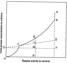
AB represents the precipitation of the less soluble contaminant. At point B, the solution becomes saturated with respect to the active component, which separates from solution along BC. At point C, the solution is saturated with the more soluble contaminant, which precipitates along CO. The slope of the tangent DE (E F /D F ) gives the specific activity of the pure enzyme. The composition of the solution at any point K on BC, in terms of the ratios of the more soluble contaminant to enzyme to less soluble contaminant is given by the lengths KL, LM, and MN respectively. The most favourable conditions for the purification of the active component will occur when the curve BCD approaches its tangent ECD as closely as possible. The precipitation conditions should therefore be manipulated to reduce the area BCE. A mathematical analysis was also provided for a three protein system, based on the fact that they all could be described by the Cohn equation. The method was then successfully applied to the final stages of purification of liver esterase. However, the method could not be applied to crude cell homogenates, due to the requirem ent of a discontinuity in the protein solubility curve as each individual protein precipitates. In a system containing a large num ber of proteins the discontinuities become indistinguishable, thus preventing the drawing of suitable tangents.
1.2.2.3 Derivative Solubility Line Method.
1.2.2.4 Fractionation Diagram s.
If the traditional method of plotting enzyme and protein solubility is considered, both the enzyme and protein concentrations are plotted per volume of initial protein solution to allow for concentration changes due to the addition of precipitant. Generally, the enzyme is assumed to follow Cohns’ equation, which gives an exponential decline in solubility. However, there is no model available for total protein that adequately describes the solubility, except for a summation of all the individual Cohn lines comprising the protein. Obviously this is an inadequate situation, although it has been suggested that the curve approaches a sigmoidal shape (Chan et al., 1986). From the diagram shown in Figure 1.5 it is possible to determine fractionation cuts to purify the required enzyme, however, it is not possible to find the degree of purification obtained or how near optimum this is.
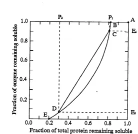
Richardson et al. (1990) provided an alternative fractionation diagram by eliminating the precipitant concentration between the enzyme and protein solubilities, and plotting the former against the latter. A typical plot is shown in Figure 1.6. The curve produced in these plots represents the process equilibrium curve. With reference to Figure 1.6, as the precipitant concentration is increased the profile remains stationary at point A, as long as both the enzyme and other proteins are totally soluble. A fterw ards, components of the total protein reach their solubility limit and the concentration decreases horizontally along AB, until at point B the solution becomes saturated with respect to the enzyme, and the solubilities of both enzyme and total protein decrease along the curve BCDE. Since the curve represents the process equilibrium, an operating tie-line can be drawn onto the diagram. In this case the operating tie-line can be obtained by considering the process parameters that give the degree of enrichm ent and the quantity of product required, namely purification factor (PF) and the yield (Y) respectively. Assuming that the quantity of enzyme and total protein in the feed stream are known, then for a tw o -cu t fractionation:
PF = (1.13)
- ^2
Y = E ^ ~ (1-14)
be viewed better if purification versus yield plots are used. These can be obtained by maximising the operating tie-line gradient for a range of yields, at different dilutions, prior to precipitation as shown in Figure 1.6. In general, the curves show a fairly rapid rise in purification as the yield is initially decreased from 100 %, indicating that there may be an advantage gained by aiming for less than 100 % recovery. If the yield is reduced much below 75 %, the slope of the curve becomes less steep and little benefit is to be gained by tra d in g -o ff yield for purification. The purification factor and yield from a fractionation diagram are found assuming an ideal equilibrium stage. In practice the true operating points will be offset due to two opposing effects:
• Soluble material lost due to occlusion in precipitated material removed in the solids underflow,
• Precipitated material remaining in the soluble stream due to the inability of industrial centrifuges to remove small, or less dense precipitate particles.
These effects can be significant for highly concentrated protein streams a n d /o r poorly dewatered precipitates. The purification and yield given by equations (1.13) and (1.14) can be adjusted to take into account the above effects as follows:
PF = ^ + f f )
(F; - + f H - (F; - + F ^ ^
Y = (F,* - + F ^ ) - (F; - + E ^ )
where * refers to the equilibrium condition, OC refers to the fraction occluded, and NR refers to the non-recovered fraction (Richardson et al., 1990).