Numerical experiments for turbulent flows
Jiˇr´ı Trefil´ık1,2,a, Karel Kozel1,2,b, and Jarom´ır Pˇr´ıhoda2,c 1 Institute of Thermomechanics AS CR, v. v. i.
2 Faculty of Mechanical Engineering, CVUT Prague
Abstract. The aim of the work is to explore the possibilities of modelling transonic flows in the internal and external aerodynamics. Several configurations were analyzed and calculations were performed using both invis-cid and viscous models of flow. Viscous turbulent flows have been simulated using either zero equation algebraic Baldwin-Lomax model and two equationk−ωmodel in its basic version and improved TNT variant. The numer-ical solution was obtained using Lax-Wendroffscheme in the MacCormack form on structured non-ortogonal grids. Artificial dissipation was added to improve the numerical stability. Achieved results are compared with experimental data.
1 Mathematical models
1.1 Navier-Stokes equations
The two-dimensional laminar flow of a viscous compress-ible liquid is described by the system of Navier-Stokes equations
Wt+Fx+Gy=Rx+Sy, (1)
where W = ρ ρu ρv e
, F=
ρu
ρu2+p
ρuv
(e+p)u
, G=
ρv ρuv
ρv2+p (e+p)v
(2) and R= 0 τxx
τxy
uτxx+vτxy+λTx
, S =
0
τxy τyy
uτxy+vτyy+λTy (3)
with shear stresses given for the laminar flow by equations
τxx= 2
3η(2ux−vy), τxy=η(uy+vx), τyy= 2
3η(−ux+2vy). (4) This system is enclosed by the equation of state
p=(κ−1) "
e−1
2ρ(u 2+v2
) #
. (5)
In the above given equations, ρdenotes density, u, v
are components of velocity in the direction of axisx, y, p
is pressure,eis total energy per a unit volume,T is tem-perature,ηis dynamical viscosity andλis thermal conduc-tivity coefficient. The parameter κ = 1.4 is the adiabatic exponent.
a e-mail:[email protected]
b e-mail:[email protected]
c e-mail:[email protected]
1.2 Reynolds averaged Navier-Stokes equations
For the modelling of a turbulent flow, the system of RANS (Reynolds Averaged Navier-Stokes) equations enclosed by a turbulence model is used. Two different turbulence mod-els with the turbulent viscosity were tested, one algebraic, Baldwin-Lomax and the two-equation k−ω model ac-cording to Wilcox. The system of averaged Navier-Stokes equations is formally the same as (1), but this time the flow parameters represent only mean values in the Favre sense, see [3]. The shear stresses are given for the turbulent flows by equations
τxx= 2
3(η+ηt)(2ux−vy), (6)
τxy=(η+ηt)(uy+vx),
τyy= 2
3(η+ηt)(−ux+2vy),
whereηt denotes the turbulent dynamic viscosity accord-ing to the Boussinesq hypothesis. The Reynolds number is
defined byRe = u∞L
η∞ and the Mach number by M = q
q a
whereq= p(u2+v2) andais the local speed of sound. All the computations were carried out using dimen-sionless variables with reference variables given by inflow values. The reference lengthLis given by the width of the computational domain.
2 Turbulence models
2.1 Baldwin-Lomax model
Algebraic models are based on the model proposed for the boundary-layer flows by Cebeci and Smith. Baldwin-Lomax model is its modification applicable for general tur-bulent shear flows. The boundary layer is divided into two regions. In the inner (nearest to the wall) part, the turbulent viscosity is given by
ηt=ρFD2κ
2y2|Ω|, (7)
DOI: 10.1051/
C
Owned by the authors, published by EDP Sciences, 2013
whereΩis the vorticity, which is in the 2D flow determined by
Ω=∂∂yu −∂v
∂x (8)
and
FD=1−exp −
y+
A+
!
. (9)
y+= u∗y
ν denotes dimensionless distance from the wall,ν= µ
ρ is kinematic viscosity,u∗ = qτ
w ρ
is so called friction
velocity andτw=µ∂∂yuy
=0.
The turbulent viscosity in the outer region is given by
ηto=αρCcpFwFk, (10)
whereCcpis a constant. FunctionFwis determined by the relation
Fw=ymaxFmax (11)
forFwbeing the maximum of the function
F=yFD|Ω| (12)
andymax the distance from the wall in which F(ymax) =
Fmaxholds and
Fk=
1+5.5 CKL
y ymax
!6 −1 . (13)
The Baldwin-Lomax model (1978) contains following val-ues of the constants: κ = 0.4, A+ = 26, α = 0.0168,
Ccp=1.6,CKL=0.3.
2.2k−ωmodel
Two-equation models are based on transport equations for two characteristic scales of turbulent motion, mostly for the turbulent energykand dissipation rate, often used in the form of specific dissipation rateω=/k. These charac-teristics are computed from transport equations. Turbulent viscosity is defined as
ηt=ρ
k
ω. (14)
The standard Wilcoxk−ωmodel is formed by the equa-tions
∂ ∂t(ρk)+
∂ ∂xj
(ρujk)=Pk+
∂ ∂xj
"
(η+σ∗ηt)∂k
∂xj #
−β∗ρkω,
(15)
∂ ∂t(ρω)+
∂ ∂xj
(ρujω)=γ
ω
kPk+
∂ ∂xj
"
(η+σηt)
∂ω ∂xj #
−βρω2, (16) where Pk = τi j∂ui/∂xj represents the production of turbulent energy. Model coefficients are given by values:
α=5/9,β=3/40,β∗ =9/100,σ =1/2 andσ∗ =1/2,
i,j∈ {1,2}.
So called TNT modification of k-ωmodel:
∂(ρk)
∂t +
∂(ρujk)
∂xj
=Pk+
∂ ∂xj
"
(µ+σkµt)
∂k
∂xj #
−β∗ρkω,
(17)
∂(ρω)
∂t +
∂(ρujω)
∂xj
=αω
kPk+
∂ ∂xj
"
(µ+σωµt)∂∂ω
xj #
−βρkω2+CD, (18) where
CD=σd
ρ
ωmax
∂k
∂xi
∂ω ∂xi
,0 !
(19)
andαω = β∗β − σ√ωκ2
β∗, κ = 0.41,β = 3 40,β
∗ = 9 100,
σω=0.5,σk=0.666.
3 Numerical methods
For the modelling of the flow cases Lax-Wendroff finite volume method scheme was used on non-orthogonal struc-tured grids of quadrilateral and hexahedral cellsDi j(k).
– Predictor step:
Win,+j1/2=W n i,j−
∆t µi,j
4
X
k=1
"
˜
Fnk−
1
ReR
n k !
∆yk− G˜nk−
1 ReS n k ! ∆xk # . (20)
– Corrector step:
Win,+j1 =
1 2(W
n i,j+W
n+1/2
i,j )−
∆t
2µi,j
4
X
k=1
"
˜
Fnk+1/2− 1 ReR
n+1/2
k !
∆yk
− G˜nk+1/2− 1 ReS
n+1/2
k !
∆xk #
+AD(Wni,j). (21)
The Mac Cormack scheme in the cell centered form was applied to solving the system of RANS equations. Con-vective termsF,Gare considered in predictor step in for-ward form and in the corrector step in upwind form of the first order of accuracy, dissipative terms in central form of the second order of accuracy. To indicate this we denote their numerical approximation as ˜F, ˜G.
The valueµi j(k) represents the surface (volume) of the cell. Figure 14 shows evaluation of derivatives on edges of cells: We imagine a virtual cell as shown in the picture. We know the values in the centers of the cells and we define the other two as a mean value of its surrounding cells. From that we extrapolate to its edges and then we apply Green’s formula.
The scheme was extended to include Jameson’s artifi-cial dissipation because of the stability of the method
AD(Win,j)=C1ψ1(Wi−n1,j−2W n i,j+W
n
i+1,j) (22) +C2ψ2(Win,j−1−2W
n i,j+W
n i,j+1), where
ψ1 = p
n i−1,j−2p
n i,j+p
n i+1,j
p n i−1,j
+ p n i,j
+ p n i+1,j
, (23)
ψ2 = p
n i,j−1−2p
n i,j+p
n i,j+1
p n i,j−1
+ p n i,j
+ p n i,j+1
Inlet boundary conditions IBCAwere used for invis-cid compressible flows; IBCBwere used for inviscid com-pressible flows. A nonzero angle of attack α1 was used only in the case of flows through DCA cascade.
On theoutletwe prescribed only pressurep2=p1and the other values were extrapolated from the flow field.
Further on there are three other types of boundary con-ditions: solid wall, symmetry axis and periodicity. These conditions are implemented by using virtual cells. Such cells adjoin from outside on the boundary cells and we prescribe values of unknowns inside of them to obtain the desired effect.
Solid wall (an inviscid flow): velocity components pre-scribed so that the sum of velocity vectors equals to zero in its tangential component.Solid wall (a viscous flow): velocity components were prescribed so that the sum of velocity vectors equals zero. In both cases the rest of un-knowns is the same in both the virtual and the boundary cell.
Symmetry axis: this condition was realized by the same way as the wall condition for an inviscid flow.
Periodicity condition: taking two corresponding seg-ments of boundary we prescribe into virtual cells of the first segment the values of unknowns contained in the bound-ary cells of the second and vice-versa.
Initial conditions were prescribed to comply with the inlet conditions.
5 Results
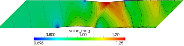
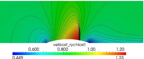
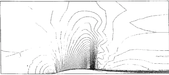
The following pictures ilustrate results obtained during the calculations. First three of them present simulation of the flow through the DCA cascade with the inlet Mach num-ber M∞ = 0.832 and angle of attackα = 0◦. Result ob-tained by employing TNT scheme shows very good agree-ment with experiagree-ment. Then similar configuration with in-let Mach numberM∞ =0.863 and angle of attackα=0◦ follows. In this case for the modelling of turbulence the Baldwin-Lomax model was used. The last configuration of this type is for inlet Mach numberM∞ =0.982 with TNT model and again there is a good agreement. Second type domain DEIW calculations follow. First there is an invis-cid flow in the same configuration as the reference result complemented by the viscous flow computation on a sym-metrical domain. But the value of Reynolds number is 10 times bigger, which might be the of cause why the separa-tion is more distinct.
Acknowledgment
The work was partly supported by by the institutional sup-port RVO 61388998 and by the grant projects GA AS CR IAA 2007 60 81, GA CR P101/10/1329, P 101/12/1271 and SGS 10/243/OHK2/3T/12.
References
1. R. Dvoˇr´ak, Transonic Flows, Academia, Prague (1986, in Czech).
2. R. Dvoˇr´ak, K. Kozel, Mathematical modelling in aero-dynamics, CTU in Prague, Prague (1996, in Czech)
3. A. Favre, Equations des gaz turbulents compressibles, Jour. de Mecanique,4, 361-390 (1965)
4. M. Feistauer, J. Felcman, I. Straˇskraba, Mathematical and Computational Methods for Compressible Flow, Oxford University Press (2003)
5. C. Hirsch, Numerical Computation of Internal and Ex-ternal Flows, Volume II, - Computational Methods for Inviscid and Viscous Flows, John Willey&Sons (1990) 6. J. Holman, J. Furst, Proceedings: Colloquium Fluid Dynamics 2008, 11-12, Institute of Thermomechan-ics, AS CR, v. v. i., Prague (2008)
7. J. Huml, J. Furst, K. Kozel, J. Pˇr´ıhoda, Proceedings: Topical Problems of Fluid Dynamics 2009, 45-48, In-stitute of Thermodynamics, AS CR, v. v. i., Prague (2009, in Czech).
8. J. Huml, J. Holman, J. Furst, K. Kozel, Proceedings: Topical Problems of Fluid Dynamics 2010, 73-76, In-stitute of Thermomechanics, AS CR, v. v. i., Prague (2010)
9. P. Poˇr´ızkov´a, Numerical Solution of Compressible Flows Using Finite Volume Method, PhD Dissertation CTU in Prague, Faculty of Mechanical Engineering, CTU in Prague, Prague (2009, in Czech).
10. J. Pˇr´ıhoda, P. Louda, Mathematical modelling of tur-bulent flow, CTU in Prague, Prague 2007 (in Czech) 11. J. ˇSimonek, K. Kozel, J. Trefil´ık, Proceedings: Topical
Fig. 3.DCA cascade, inviscid flow,M∞=0.88,α=0.6◦, Mach number isolines
Fig. 4.DCA cascade, viscous flow,M∞=0.88,α=0.6◦,Re=107,k−ωmodel, Mach number isolines
Fig. 5.DCA cascade, viscous flow,M∞=0.89,α=0.5◦,Re=107,k−ωmodel (TNT variant), Mach number isolines
Fig. 6.Experimental data,M∞=0.832,α=0◦
Fig. 7.DCA cascade, inviscid flow,M∞=0.98,α=3.0◦, Mach number isolines
Fig. 9.Experimental data,M∞=0.863,α=0◦
Fig. 10.DCA cascade, viscous flow,M∞=1.07,α=2.3◦,Re=107,k−ωmodel (TNT variant), Mach number isolines
Fig. 11.Experimental data,M∞=0.982,α=0◦
Fig. 13.symmetric DEIW configuration, viscous flow,M∞=0.775,α=0◦,Re=106,k−ωmodel (TNT variant), Mach number isolines