ISSN (e): 2250-3021, ISSN (p): 2278-8719
Vol. 04, Issue 01 (January. 2014), ||V5|| PP 38-48
Optimum Design of a Hybrid PV/Wind Energy System Using
Genetic Algorithm (GA)
Satish Kumar Ramoji
1, Bibhuti Bhusan Rath
2, D.Vijay Kumar
3 1(PG Student, Dept. of E.E.E., AITAM, Tekkali, Andhra Pradesh, India, 2(Assoc. Prof., Dept. of E.E.E., AITAM, Tekkali, Andhra Pradesh, India, 3(Prof. & H.O.D., Dept. of E.E.E., AITAM, Tekkali, Andhra Pradesh, India,
Abstract: - In this paper, a new approach of optimum design for a Hybrid PV/Wind energy system is presented in order to assist the designers to take into consideration both the economic and ecological aspects. When the stand alone energy system having photovoltaic panels only or wind turbine only are compared with the hybrid PV/wind energy systems, the hybrid systems are more economical and reliable according to climate changes. This paper presents an optimization technique to design the hybrid PV/wind system. The hybrid system consists of photovoltaic panels, wind turbines and storage batteries. Genetic Algorithm (GA) optimization technique is utilized to minimize the formulated objective function, i.e. total cost which includes initial costs, yearly replacement cost, yearly operating costs and maintenance costs and salvage value of the proposed hybrid system. A computer program is designed, using MATLAB code to formulate the optimization problem by computing the coefficients of the objective function. The method mentioned in this article is proved to be effective using an example of hybrid energy system. Finally, the optimal solution is received using Genetic Algorithm (GA) optimization method.
Keywords: - Battery, Genetic Algorithm, Hybrid PV/Wind energy system, Optimization, and wind energy
I.
INTRODUCTION
Global environmental concerns and the ever-increasing need for energy, coupled with a steady progress in renewable/green energy technologies, are opening up new opportunities for utilization of renewable energy resources. In particular, advances in wind and photovoltaic (PV) generation technologies have increased their use in wind-alone, PV-alone, and hybrid PV-wind configurations. Moreover, the economic aspects of these renewable energy technologies are sufficiently promising at present to include the development of their market
II.
HYBRID
SYSTEM
STRUCTURE
Fig. -1 shows the proposed optimization procedure of the PV-Wind hybrid system based on high resolution solar irradiance including the cost analysis.
Figure -1: Flowchart of the proposed optimization methodology
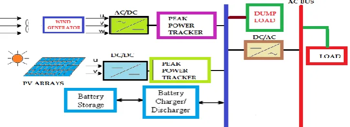
The suggested approach employs a technical assessment in conjunction with cost-per-watt to select and size the PV panel, wind turbine, and battery storage in order to determine the system that would guarantee a reliable energy supply with the lowest investment. Figure -2 shows the general schematic of the hybrid system. The system can be divided into three main stages; the first stage is the generation which includes the PV and wind systems. The second stage is the conversion and storage energy system. The conversion system includes the DC/DC converter for the PV system, the AC/DC converter for the wind generators, and DC/AC inverter which is connected to the DC bus and supplies the 440 V AC power to the load. The third stage is the grid connected load, where the 60% of the demand is supplied by the hybrid system.
III.
METEOROLOGICAL
AND
LOAD
DATA
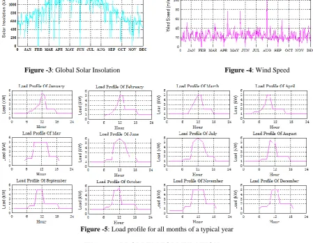
The proposed method is to optimally size a PV-wind hybrid energy system to electrify a residential remote area household near to latitude is 39.74˚ N, Longitude 105.18˚ W, Time Zone: GMT7, Elevation: -1829 m. MIDC/NREL Solar Radiation Research Laboratory (BMS) is a good source for the long-term monthly average daily solar radiation data (incident on both horizontal and south-facing PV array tilted by the latitude angle ϕ of the site) and wind speed data (measured at 42 feet/12.8 m height in the site). The proposed method requires a recorded long-term wind speed data and global insolation data (incident on a south-facing PV array tilted by the site latitude angle ϕ) for every day of each month in a period of 1 year. Figures 3 and 4 show these data (i.e., the global solar insolation and wind Speed, respectively) for every month in a typical year. Figure 5 illustrates the considered residential remote area load profile, during the 12 months of the year.
Figure -3: Global Solar Insolation Figure -4: Wind Speed
Figure -5: Load profile for all months of a typical year
IV.
PROBLEM
FORMULATION
The major concern in the design of the proposed PV-wind hybrid energy system is to determine the size of each component participating in the system so that the load can be economically and reliably satisfied. Hence, the system components are found subject to: 1. minimizing the total cost (CT) of the system, 2.ensuring
that the load is served according to certain reliability criteria. The objective function (CT) is to be minimized,
and this cost function is generated by the summation of the present worth (PWs) of all the salvage values of the equipment, the yearly operation and maintenance costs, the initial or capital investments, and the replacement costs of the system components. Thus, the objective function can be formulated as:
(1) Where the index k is to account for PV, wind, and batteries; Ik is the capital or initial investment of
each component k; RPWk is the PW of the replacement cost of each component k; OMPWk is the PW of the
k. The constraints that ought to be met, while minimizing the objective function CT, should ensure that the load
is served according to some reliability criteria.
IV.1. Basic Economic Considerations
As Equation (1) suggests, the PWs of some annual payments as well as of salvage values are needed. Thus, assuming a life horizon of N years for the project, an interest rate r, and an inflation rate j (caused by increases in prices), the different PWs can be calculated as follows [16]: -
IV.1.1: Salvage Value
If a component has a salvage value of S (Rs.) at present (because it is reaching the end of its life cycle), then the salvage value of the component is expected to be S(1+j)N (i.e., N years from now provided that the component is put in service at the present time). The PW of S(1+j)Ntaking the interest rate into consideration, is
(2) Let fac1= , then SPWk=Sk facl, for all components k in the hybrid system.
IV.1.2: Operation and Maintenance
If the operating and maintenance cost of a component is OM (Rs./year), then this tends to escalate each year at a rate not necessarily equal to the general inflation rate. Thus, for an escalation rate es the operation and maintenance costs incurred at year y will be OM (1+es)y, and having a PW of : OM (1+es)y/(1+r)y (3)
The summation of the PWs of all the annual payments is, thus, given by:
OMPW = OM. = OM. fac2 (4)
Where fac2 represents a geometric progression, and is given by:
fac2 = ( ). [1-( ], r
N, r = es (5)
Hence, OMPWk=OMk. fac2, for all components k in the system. Note that other PW calculations will be treated
in a similar manner throughout the analysis of each component.
IV.2. Total Cost Coefficients IV.2.1: The PV Array
Assuming the design variable, in case of the PV array, to be the total array area APV in square meters. This area is constrained by both the maximum available area for the PV
Array (e.g., the roof surface of buildings) and the budget preset for the PV modules. With an initial cost of αPV
(Rs./m2), the total initial investment would be:
I1 = αPV . APV (6)
Note, here, that if the project life span is assumed to be the same as the PV array lifetime, then the replacement cost of the PV modules will be negligible (i.e.,RPW1=0). With a yearly operation and maintenance cost of αOMPV
(Rs./m2/year), the total yearly operation and maintenance cost would be OM1=αOMPV.APV. Thus, the global PW
of the yearly operation and maintenance cost would be
OMPW1= αOMPV . APV . fac2 (7)
The salvage value can be found by multiplying the selling price per square meter SPV by the area APV, and the
PW of the selling price would be
SPW1= SPV . APV . fac1 (8)
In summary, the PWs of the PV array costs are:
I1+RPW1 = αPV . APV = c1 . APV
OMPW1 = αOMPV . APV . fac2 = c2 . APV
SPW1= SPV . APV . fac1 = c3 . APV
IV.2.2: The Wind Turbine
end. The number of times, within N years, a wind turbine is needed is Xw=N/Lw (rounded to the greater integer). If αw is the price in Rs./m2 at present, the price at year y would be αw.(1 +es)y having the PW of αw.(1
+es)y/(1+r)y. Thus, the PW of all the initial and replacement investments in wind turbines is
I2+RPW2 = αw . Aw (9)
Where es is the escalation rate, r is the interest rate, Lw is the lifetime of wind turbines, and Xw is the number of times wind turbines are purchased. Note that if Xw equals 1 (i.e., the life span of the wind turbines is greater than or equal to that of the whole project), then RPW2=0 and I2=αw . Aw (since the wind turbines are
bought once at the beginning of the project). With a yearly operation and maintenance cost of αOMw
(Rs./m2/year), the total yearly operation and maintenance cost would be OM2=αOMw.Aw, and the PW of all the
yearly costs would be:
OMPW2= αOMw . Aw . fac2 (10)
The salvage value of the wind turbine is assumed to decrease linearly from αw (Rs./m2) to Sw (Rs./m2),
when the wind turbine operates along its lifetime Lw (i.e., from its installation to the end of its lifetime,
respectively). If the project life comes to an end before the wind turbines have reached the end of their life span, then the wind turbines could be sold at Spw (Rs/m2), which is a value greater than Sw.
Spw = . Years + αw (11)
Where “years” indicates the number of years of operation between the installation of the last wind turbine and the end of the project life span. Therefore, the PW of all the salvage values is found by:
SPW2 = Sw . Aw + Spw . Aw (12)
If N (i.e., the life span of the project) is a multiple of that of the wind turbines Lw, then Equation (12) can be reduced to
SPW2 = Sw . Aw (13)
In summary, the PWs of the wind turbine are:
I2+RPW2 = αw . Aw = c4 . Aw
OMPW2= αOMw . Aw . fac2 = c5 . Aw
SPW2=Sw . Aw + Spw . Aw = c6 . Aw
IV.2.3: The Storage Batteries
The design variable in the case of storage batteries is their capacity Cb in kilo watt hours. As in the case of wind turbine, the lifetime of a battery Lb is expected to be less than that of the whole project. Hence, batteries of capacity Cb are to be purchased at regular intervals of Lb. The total PW of the capital and replacement investments in batteries is given by:
I3+RPW3 = αb . Cb (14)
Where Lb is the battery lifetime, Xb is the number of times batteries should be purchased during the project lifetime: Xb=N/Lb (rounded to the greater integer), and αb is the capital cost in (Rs./kWh). The salvage value of the batteries is assumed to be negligible. With a yearly operation and maintenance cost of αOMb (Rs./kWh/year),
the total yearly operation and maintenance cost would be OM3=αOMb.Cb, and the PW of all the yearly costs
would be:
OMPW3 = αOMb . Cb . fac2 (15)
In summary, the PWs of the battery costs are:
I3+RPW3 = αb . Cb = c7 . Cb
OMPW3 = αOMb . Cb . fac2 = c8 . Cb
SPW3 = 0
IV.3. System Modeling
IV.3.1: Modeling of the PV Array
For a PV array having an efficiency ηPV and area APV (m2), the output power PPV (kW), when subjected to the available solar insolation R (kW/m2) on the tilted surface, is given by [11]
PPV = R . APV . ηPV (16)
Here, the insolation R incident on the PV array is defined in Figure 3.
IV.3.2: Modeling of the WTG
A WTG produces power Pw when the wind speed V is higher than the cut-in speed Vci and is shut-down when V is higher than the cut-out speed Vco. When Vr <V<Vco (Vr is the rated wind speed), the WTG produces rated power Pr. If Vci<V<Vr, the WTG output power varies according to the cube law. The following equations are to be used in order to model the WTG [7, 13]
(17) Where
Pr = CP ρair Aw (18)
In the above equation, Cp, ρair, and Aw are the power coefficient, air density, and rotor swept area, respectively. As the available wind speed data Vi (see Figure 4) were estimated at a height Hi=42 feet/12.8 m, then to upgrade these data to a particular hub height H, the following equation is commonly used [1, 7]
(19)
Where V is the upgraded wind speed at the hub height H and a is the power-law exponent (≈1/7 for open land).
IV.3.3: Modeling of the Storage Battery
At any hour t, the state of charge of the battery [SOC (t)] is related to the previous state of charge [SOC (t – 1)] and to the energy production and consumption situation of the system during the time from t –1 to t. During the charging process, when the battery power PB flows toward the battery (i.e., PB>0), the available battery state of charge at hour t can be described by:
SOC (t) = SOC (t-1) + (20)
Where Δt is the simulation step time (which is set equal to 1 hour), and Cbis the total nominal capacity of the battery in kilowatt-hours. On the other hand, when the battery power flows outside the battery (i.e., PB<0), the
battery is in discharging state. Therefore, the available battery state of charge at hour t can be expressed as: SOC (t) = SOC (t-1) - (21)
To prolong the battery life, the battery should not be over discharged or overcharged. This means that the battery SOC at any hour t must be subject to the following constraint:
(1 - ) ≤ SOC (t) ≤ (22)
Where DODmax and SOCmax are the battery maximum permissible depth of discharge and SOC, respectively.
V.
SYSTEM RELIABILITY AND SIMULATION
First of all, it is assumed, in this work, that the peak power trackers, the battery charger/discharger, and the distribution lines are ideal (i.e., they are lossless). Also, it is assumed that the inverter efficiency ηinv is constant; the battery charge efficiency ηb is set to equal to the manufacturers’ round-trip efficiency, and the battery discharging efficiency is set to be 1. The total generated power by the PV array and WTG for hour t,
Pg(t), can be expressed as
Pg (t) = PPV (t) + Pw (t) (23)
It is to be noted that the desired load demand at any hour t, PL∗(t), may or may not be satisfied according to the
corresponding values of the total generated power Pg(t) and the available battery SOC(t) at that hour. The proposed energy management of the PV-wind hybrid system can be summarized as follows:
If [Pg(t)>PL∗(t)/ηinv] and [SOC(t –1)<SOCmax] then satisfy the load and charge the battery [using Equation (20)] with the surplus power [PB(t)=(Pg(t)− PL∗(t)/ηinv)ηb]. Afterwards, check if [SOC(t)≥SOCmax] then stop
battery charging, set SOC(t)=SOCmax, and dump the surplus power (PDump(t)=Pg(t)−[PL∗(t)/
If [Pg(t)>PL∗(t)/ηinv] and [SOC(t–1)≥SOCmax] then stop charging the battery, satisfy the load, and dump the surplus power [PDump(t)= Pg(t)− PL∗(t)/ηinv].
If [Pg(t) =PL∗(t)/ηinv] then satisfy the load only.
If [Pg(t)<PL∗(t)/ηinv] and [DOD(t–1)<DODmax] then satisfy the load by discharging the battery [using
Equation (21)] to cover the deficit in load power [PB(t)= PL∗(t)/ηinv - Pg(t)]. Afterwards, check if
[DOD(t)≥DODmax] then stop battery discharging, set DOD(t)=DODmax, and calculate the deficit in load
power (Pdeficit(t)=PL∗(t)-[Pg(t)+ 1000×Cb/Δt×( SOC(t−1) −(1−DODmax))] ηinv.
If [Pg(t)<PL∗(t)/ηinv] and [DOD(t–1) ≥DODmax] then stop battery discharging and [Pdeficit(t)= PL∗(t) − Pg(t).
ηinv.
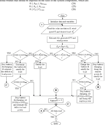
As it is assumed, in this work, the simulation step time Δt is equal to 1 h and the generated PV and wind powers are constants during Δt Then, the power is numerically equal to the energy within Δt. A flowchart diagram for this program is shown in Figure 6. The input data for this program consist of mean hourly global insolation on a tilted array R, mean hourly wind speed Vi, and desired load power during the year PL∗. Note, here, that for every
configuration of the proposed PV-wind hybrid system, this program simulates the system. There are three additional bounds that should be imposed on the sizes of the system components, which are:
0 ≤ APV ≤ APVmax (24)
0 ≤ Aw ≤ Aw max (25)
0 ≤ Cb ≤ Cb max (26)
VI.
FINAL FORM AND GA OPTIMIZATION
At this stage, the optimization problem can be written in its final form as follows:1. Minimize the cost function CT
(c1+c2-c3). APV + (c4+c5-c6). AW + (c7+c8).Cb (27) 2. Subject to:
0 ≤ APV≤ APVmax
0 ≤ Aw≤ Aw max
0 ≤ Cb≤ Cb max (28)
To solve the above optimization problem, GA is proposed, where, in this work, the Genetic Algorithm Code under MATLAB software is utilized for solving the previous optimization problem. GA contains the elitist approach. This means that a solution cannot degrade from one generation to the next, but that best individual of a generation is copied to the next generation without any changes being made to it. To use the GA, for solving the formulated optimization problem, a M-file (MATLAB Code) has written, to compute the values of the
objective function (or called fitness function).The M-file has to be written to accept a vector (i.e., individual) whose length is the number of independent variables for the objective function and return the corresponding scalar values of the objective function (i.e., cost). In this work, the individual of the considered optimization problem contains three variables (or genes), which are: APV, Aw, and Cb. The used GA is based upon using the
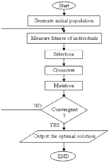
flowchart of Figure 7, to yield the optimal solution. Initially, the GA selects individuals at random from the current population to be parents and uses them to produce the children for the next generation by using the three main operations, which are the selection, crossover, and mutation operations. Then, it can repeatedly modify a population of individual solutions, where, over successive generations, the population evolves toward an optimal solution. Note, here, that the used different settings in the GA are 100 individuals for the population size, the stochastic uniform function for the selection operation, the scattered crossover function (with a crossover probability of 80%) for the crossover operation, the adaptive feasible mutation function (with a probability rate of 1%) for the mutation operation, and an elite individual. At the same time, it is to be noted that the additional three bounds of Equation (28) can be entered directly in the dedicated positions of the GA.
Figure -7: Flow-chart of the Genetic Algorithm (GA)
VII.
APPLICATION RESULTS AND DISCUSSION
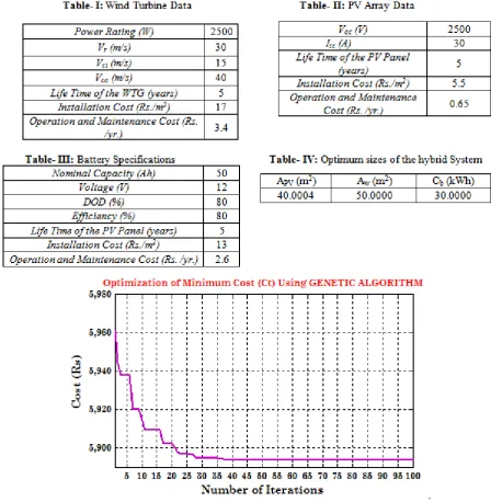
installation cost of each component have been set at 0-1% and 5-10% respectively of the corresponding cost. The life time of Wind Turbine, PV panel and Battery is considered to be 5 years. Since the tower heights of wind turbines affect the results significantly, 12.8m meter high tower at an elevation of 1829m is chosen. The minimization of the system total cost is achieved by selecting an appropriate system configuration. In table IV, it indicates the resulted optimum sizes of the different components included in the hybrid system. The corresponding fitness function optimization (i.e., minimization of the system cost in rupees) along the successive generations of the GA is shown in Figure 8, which indicates that the system is optimized after forty iterations only.
. Figure -8: Optimization of the Objective function using GA
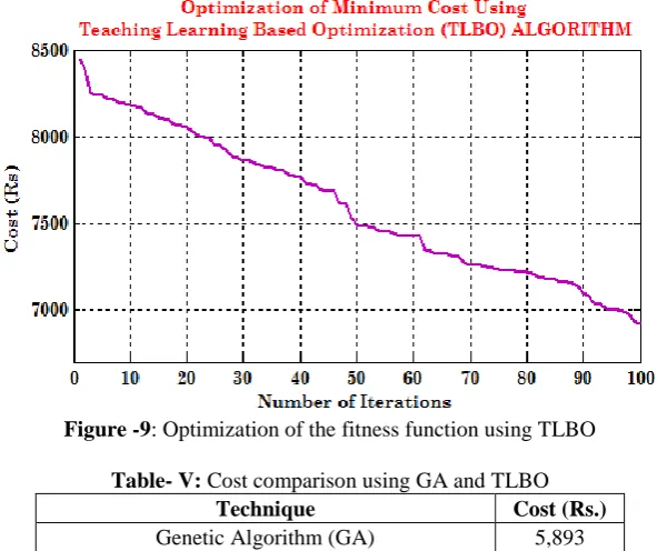
simulates the traditional teaching-learning phenomenon of the classroom. The algorithm simulates two fundamental modes of learning: (i) through teacher (known as teacher phase) and (ii) interacting with the other learners (known as the learner phase). TLBO is a population based algorithm where a group of students (i.e. learners) is considered as population and the different subjects offered to the learners is analogous with the different design variables of the optimization problem. The grades of a learner in each subject represent a possible solution to the optimization problem (value of design variables) and the mean result of a learner considering all subjects corresponds to the quality of the associated solution (fitness value).The best solution in the entire population is considered as the teacher. In another M-file a MATLAB code has written for proposed hybrid PV/Wind energy system using Teaching Learning Based Optimization (TLBO) algorithm. The corresponding fitness function optimization (i.e., minimization of the system cost in rupees) along the successive iterations of the TLBO is shown in Figure 9, which indicates that the system is not optimized even after hundred iterations.
Figure -9: Optimization of the fitness function using TLBO
Table- V: Cost comparison using GA and TLBO Technique Cost (Rs.) Genetic Algorithm (GA) 5,893 Teaching Learning Based Optimization (TLBO) 6,968
Figure 10, 11, and 12 illustrates the generated PV power, wind power, and the total generated power of the suggested PV-wind hybrid system, for every month during the year.
Figure-10: PV Power Figure-11: Wind Power
VIII.CONCLUSIONS
This paper presents a GA-based optimization technique to optimally size a proposed PV-wind hybrid energy system, incorporating a storage battery. The optimization problem is formulated, in this work, to achieve a minimum total cost for the system components and to ensure that the load is served reliably. The results yield that the GA converges very well and the proposed technique is feasible for sizing either of the PV-wind hybrid energy system, stand-alone PV system, or stand-alone wind system. In addition, the proposed technique is able to be adjusted if insolation, wind speed, load demand, and initial cost of each component participating in the system are changed. The results yield, also, that the PV-wind hybrid energy systems are the most economical and reliable solution for electrifying remote area loads.
REFERENCES
[1]. Kellogg, W.D., M.H. Nehrir, G. Venkataramanan, and V. Gerez. 1998. Generation unit sizing and cost analysis for stand-alone wind, photovoltaic, and hybrid wind/PV systems. IEEE Trans. on Energy Conversion 13(1): 70–75.
[2]. Gupta, A., R.P. Saini, and M.P. Sharma. 2007. Design of an optimal hybrid energy system model for remote rural area power generation. In Proceedings of the IEEE International Conference on Electrical Engineering (ICEE 2007), Lahore, Pakistan, 1–6.
[3]. Hongxing, Y., Z. Wei, and L. Chengzhi. 2009. Optimal design and techno-economic analysis of a hybrid solar–wind power generation system. Applied Energy 86: 163–169.
[4]. Roman, E., R. Alonso, P. Ibanez, S. Elorduizapatarietxe, and D. Goitia. 2006. Intelligent PV module for grid-connected PV systems. IEEE Transactions on Industrial Electronics 53(4):1066–1073.
[5]. Colle, S., S. Luna, and R. Ricardo. 2004. Economic evaluation and optimization of hybrid diesel/PV systems integrated to utility grids. Solar Energy 76: 295–299.
[6]. Wies, R.W., R.A. Johnson, A.N. Agrawal, and T.J. Chubb. 2005. Simulink model for economic analysis and environmental impacts of a PV with diesel-battery system for remote villages. IEEE Transactions on Power Systems 20(2): 692–700.
[7]. Borowy, B.S., and Z.M. Salameh. 1996. Methodology for optimally sizing the combination of a battery bank and PV array in a wind/PV hybrid system. IEEE Transactions on Energy Conversion 11(2): 367– 375.
[8]. Prasad, A.R., and E. Natarajan. 2006. Optimization of integrated photovoltaic-wind power systems with battery storage. Energy 31: 1943–1954.
[9]. Shaahid, S.M., and M.A. Elhadidy. 2008. Economic analysis of hybrid photovoltaic-diesel-battery power systems for residential loads in hot regions-a step to clean future. Renewable and Sustainable Energy Reviews 12: 488–503.
[10]. Ai, B., H. Yang, H. Shen, and X. Liao. 2003. Computer aided design of PV/wind hybrid system.
Renewable Energy 28: 1491–1512.
[11]. Diaf, S., D. Diaf, M. Haddadi, and A. Louche. 2007. A methodology for optimal sizing of autonomous hybrid PV/Wind system. Energy Policy 35: 5708–5718.
[12]. Senjyu, T., D. Hayashi, N. Urasaki, and T. Funabashi. 2006. Optimum configuration for renewable generating systems in residence using genetic algorithm. IEEE Transactions on Energy Conversion
21(2): 459–466.
[13]. Yang, H., L. Lu, and W. Zhou. 2007. A novel optimization sizing model for hybrid solar-wind power generation system. Solar Energy 81: 76–84.
[14]. Karaki, S.H., R.B. Chedid, and R. Ramadan. 1999. Probabilistic performance assessment of autonomous solar-wind energy conversion systems. IEEE Transactions on Energy Conversion 14(3): 766–772. [15]. Chedid, R., H. Akiki, and S. Rahman. 1998. A decision support tech. for the design of hybrid PV/wind
systems. IEEE Transactions on Energy Conversion 13: 76–82.
[16]. Sweelem, E.A., and A.A. Nafeh. 2006. A linear programming technique for optimally sizing a PV-diesel-Battery hybrid energy system. Al-Azhar University Engineering Journal 9(3): 705–716.
[17]. Xu Daming, Kang Longyun, Cao Binggang, “Stand-alone hybrid wind/PV power system using the NSGA2,” Acta energiae solaris sinica, vol. 27, no. 6, pp.593-598, 2006.