R E S E A R C H
Open Access
An extended triangulation to the
Marching Cubes 33 algorithm
Lis Custodio
1*, Sinesio Pesco
2and Claudio Silva
3Abstract
The Marching Cubes algorithm is arguably the most popular isosurface extraction algorithm. Since its inception, two problems have lingered, namely, triangle quality and topology correctness. Although there is an extensive literature to solve them, topology correctness is achieved in detriment of triangle quality and vice versa. In this paper, we present an extended version of the Marching Cubes 33 algorithm (a variation of the Marching Cubes algorithm which guarantees topological correctness), called Extended Marching Cubes 33. In the proposed algorithm, the grid vertex are labeled with “+,” “−,” and “=,” according to the relationship between its scalar field value and the isovalue. The inclusion of the “=” grid vertex label naturally avoids degenerate triangles. As an application of our method, we use the proposed triangulation to improve the quality of the triangles in the generated mesh while preserving its topology as much as possible.
Keywords: Isosurface extraction, Marching Cubes 33, Mesh quality, Extended lookup table
Introduction
The isosurface extraction algorithms are a powerful tool in the interpretation and visualization of volumetric data. Among the isosurface extraction algorithms, the March-ing Cubes, originally proposed by Lorensen and Cline [1] in 1987, stands out for its simplicity, robustness, and speed. An isosurface provides a mechanism for under-standing the structure of volumetric data, which is why an accurate representation is needed to interpret data correctly.
Given a scalar fieldf : D⊂ R3 →Rand a scalar value α, the isosurfaceSα, associated toα, consists of the set of the pointsx∈R3such thatf(x)=α:
Sα=x∈R3|f(x)=α. (1)
In the computational process of isosurfaces extraction, the scalar field f is sampled on the vertices of a three-dimensional rectilinear grid and linearly interpolated on the edges, faces, and interior of the cubes of this grid (see Fig.1).
*Correspondence:[email protected]
1Computational Modeling Department, Polytechnic Institute at the Rio de
Janeiro State University, Rio de Janeiro, Brazil
Full list of author information is available at the end of the article
Thus, let g : D ⊂ R3 → R be a function that interpolates the scalar fieldf in each cell of the grid:
g(x,y,z)=(1−x)(1−y)(1−z)f(v0)+(1−x)(1−y)zf(v4) +(1−x)y(1−z)f(v3)+(1−x)yzf(v7) +x(1−y)(1−z)f(v1)+x(1−y)zf(v5) +xy(1−z)f(v2)+xyzf(v6),
where we consider, without loss of generality, a unit cube, given a scalar valueα, we want to construct, within each cube, a three-dimensional model (usually constituted by a triangular mesh) that correctly represents the geometry and topology of the isosurface:
¯
Sα=x∈R3|g(x)=α. (2)
The Marching Cubes is the most popular isosurface extraction technique, and it has been an active research topic for decades. The premise of algorithm is to divide the input volume into a discrete set of cubes. By assuming linear reconstruction filtering, each cube, which contains a piece of a given isosurface, can easily be identified because the sample values at the cube vertices must span the target isosurface value. For each cube containing a section of the isosurface, a triangular mesh that approx-imates the behavior of the trilinear interpolant in the interior cube is generated.
Fig. 1Illustration of a cube in the grid
LetHbe a rectilinear grid in a volumetric data domain D, such thatf : D ⊂ R3 → Ris the scalar field repre-sented by these data andαis the desired isovalue. A vertex viof a cube inHis classified aspositiveiff(vi) ≥ αand
negativeiff(vi) < α. Since there are eight vertices in each
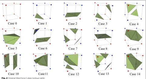
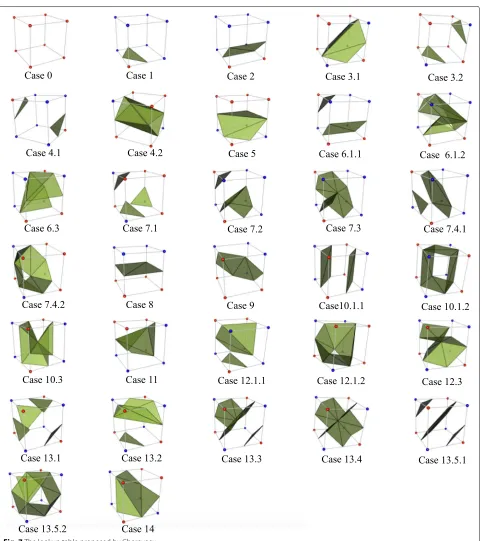
cube, there are 28 = 256 possible ways that the isosur-face can intersect the cube. Considering the symmetries in the cube, these 256 cases are reduced to 14 patterns, with 14 cases, which supposedly would cover the possi-ble behaviors of the trilinear interpolant inside the cube (see Fig.2).
However, due to the existence of ambiguities in the trilinear interpolant behavior in the cube faces and
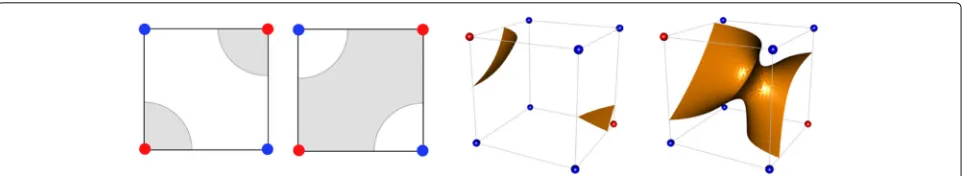
interior, the meshes extracted by the Marching Cubes presented discontinuities and topological issues. Given a cube of the grid, a face ambiguity occurs when its face vertices have alternating signs, that is, the vertices of one diagonal on this face are positive and the ver-tices on the other are negative. Observe that in this case, the signs of the face vertices are insufficient to determine the correct way to triangulate the isosurface. Similarly, an interior ambiguity occurs when the signs of the cube vertices are insufficient to determine the correct surface triangulation, i.e., when multiple trian-gulations are possible for the same cube configuration (see Fig.3).
Fig. 3Right: case 4 ambiguity. The interior ambiguity test proposed by Chernyaev is used choose the correct configuration. Left: face ambiguity. The Asymptotic Decider is used to resolve the ambiguity
The popularity of the Marching Cubes and its widespread adoption resulted in several improvements in the algorithm to deal with the ambiguities and to correctly track the behavior of the interpolant. Dürst [2] in 1988 was the first to note that the triangulation table proposed by Lorensen and Cline [1] was incomplete and that cer-tain Marching Cubes cases allow multiple triangulations. Later, Nielson and Hamann [3] in 1991 observed the exis-tence of ambiguities in the interpolant behavior on the face of the cube. They proposed a test called Asymptotic Decider to correctly track the interpolant on the faces of the cube. In fact, as observed by Natarajan [4] in 1994, this ambiguity problem also occurs inside the cube. In his work, the author proposed a disambiguation test based on the interpolant critical points and added four new cases to the Marching Cubes triangulation table (subcases of the cases 3, 4, 6, and 7). At this point, even with all the improvements proposed to the algorithm and its triangu-lation table, the meshes generated by the Marching Cubes still had topological incoherencies.
The Marching Cubes 33, proposed by Chernyaev [5] in 1995, is one of the first isosurface extraction algorithms intended to preserve the topology of the trilinear inter-polant. In his work, Chernyaev extends to 33 the number of cases in the triangulation lookup table (see Fig.7). He then proposes a different approach to solve the interior ambiguities, which is based on the Asymptotic Decider. Later, in 2003, Nielson [6] proved that Chernyaev’s lookup table is complete and can represent all the possible behav-iors of the trilinear interpolant, and Lewiner et al. [7] pro-posed an implementation to the algorithm. More recently Custodio et al. [8] in 2013 and Grosso [9] in 2016 worked to guarantee topological correctness of the meshes gener-ated by the Marching Cubes.
The Marching Cubes is considered robust, simple, and with a low computational cost. These characteristics have made it the most popular isosurface extraction algorithm. However, the weakness of the algorithm lies on the quality of the resulting mesh. The triangulation generated by the Marching Cubes is characterized by a large number of degenerate and skinny triangles. The degenerations are caused by the way the algorithm classifies the vertices of
the grid; a vertex is classified aspositiveif it has a scalar value equal or greater than the isovalue, andnegativeif it has a scalar value less than the isovalue. Note that if a ver-tex has scalar value equal to the isovalue, it is classified as a positive vertex. Consequently, its three incidents edges will be classified as intersected edges (edges intersected by the isosurface), and a triangle with its three vertices in the same point (the vertex of the grid which the scalar field value match with the isovalue) is created. A skinny trian-gle is generated when two of its vertices are close to a grid vertex while the third vertex is far from this vertex.
To avoid the creation of degenerate triangles by the Marching Cubes algorithm, Raman and Wenger [10] in 2008 propose a lookup table that includes grid vertices with labels “+,” “−,” and “=,” according to the relationship of the isovalue with its scalar value. This classification of the grid naturally avoids the generation of degener-ate triangle. The authors also present the application of the extended lookup table to improve the quality of the triangulation on the resulting mesh.
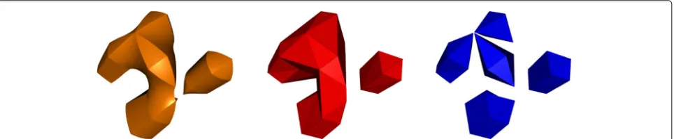
In their work, Raman and Wenger [10] opt to use the lookup table proposed by Montani et al. [11] in 1994 as reference to their triangulation process, and the extended lookup table proposed inherits some limitations of Montani et al. work, namely, it covers only 23 of the 33 possible behavior of the trilinear interpolant in the interior of the cube. Hence, the mesh produced by both Montani et al. and, consequently, by the Raman and Wenger lookup tables cannot represent the topology of the trilinear interpolant correctly. Figure 4 shows an example of topological inconsistencies in the meshes gen-erated by Raman and Wenger’s method. The orange mesh shows the expected isosurface extracted from a 5×5 ×5 randomly sampled grid H, which contains some voxels with ambiguous configurations. The blue mesh was extracted fromGby the algorithm proposed by Raman and Wenger. The method fails to represent the topology of the trilinear interpolant correctly. The red mesh was extracted by the method proposed in this work.
Fig. 4Left: isosurface generated by randomly sampling a 5×5×5 grid. Some of the voxels contain ambiguous configurations. Middle: mesh generated by our method tends to preserve the topology and produces good quality triangles. Right: mesh extracted by the Raman and Wenger method fails to correctly represent the isosurface topology
(top), the single behavior covered by the Montani et al. lookup table (bottom left), and the missing triangulations (bottom middle and right). The same issue applies to other ambiguous configurations.
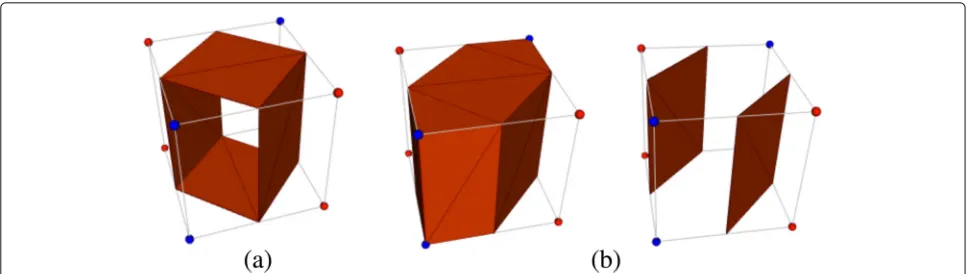
Figure 6 illustrates what happens when Raman and Wenger’s method tries to construct the triangulation of a configuration that the base lookup table proposed by Montani et al. does not cover it. In this lookup table, there is no possibility of a “tunnel” crossing the cube in case 10 (see Fig. 7); hence, the topology of Raman and Wenger’s method does not match the topology of the trilinear interpolant. Note that the problem here is more complicated than simply replacing the Raman and Wenger’s base lookup table with an extended one. In fact, the triangulation presented in Fig. 6a cannot be produced by the method proposed by Raman and Wenger.
To solve the problem of degenerate triangles and also to preserve the topological correctness of the resulting mesh as much as possible, we propose a method to construct an extended triangulation to the Marching Cubes 33. The challenge is to build an extended triangulation to the com-plex cases present in the topologically correct lookup table proposed by Chernyaev [5] (see Fig.7). In addition, we apply our method to improve the quality of the triangula-tion in the resulting mesh. As we describe in the following sections, the key of our method is to construct the tri-angulation respecting the regions defined by the trilinear interpolant inside the cube.
Our contributions are:
• A method to build an extended triangulation to the Marching Cubes 33 algorithm. The proposed method allows vertices of the grid to be part of the
Fig. 6 aThe correct triangulation for the case 10.2 (the interpolant inside the cube is homeomorphic to a cylinder).bThe triangulation method proposed by Raman and Wanger. (Left) A triangulation of the convex hull of positive and edge intersection points is built. (Right) Then, the triangles coplanar to the faces of the cube are removed
triangulation, which avoids degenerate triangles, so common in the Marching Cubes mesh.
• An algorithm to avoid the skinny triangle in the resulting mesh. It is an algorithm similar to the proposed by Raman and Wenger [10], but as shown in “Improving the triangulation quality of the final mesh” section, the mesh generated by our method better preserves the topology of the trilinear interpolant.
In addition, to better represent our results, we made our figures executable. In the pdf version of this work, you have access to an interactive visualization found in the
project pageby simply clicking on the figures.
Related work
In 2000, Lachaud and Montanvert [12] and Bhaniramka et al. [13] independently proposed an algorithm to gener-ate a Marching Cubes lookup table in higher dimension. In both methods, the ambiguities of the trilinear inter-polant in the interior of the cube are not considered in constructing the triangulation, which leads to topologi-cal inconsistencies in the generated mesh. Later, in 2004, Bhaniramka et al. [14] proposed the use of convex hulls in the isosurface construction.
In 2008, Raman and Wenger [10], based on the Bhaniramka et al.’s [14] work, proposed an algorithm to construct an extended lookup table which allows the vertices of the grid to be part of the triangulation. By using grid vertices in the triangulation, the algorithm avoids the creation of degenerate triangles. The pro-posed algorithm is also used to improve the quality of the generated mesh: modifications on the value of the scalar fields on the vertices of the grid are used to avoid the creation of skinny triangles. However, as dis-cussed in the previous section, the proposed method cannot correctly represent the topology of the trilinear interpolant.
Wang et al. [15] proposed in 2014 a method to address the problem of needing to access the cubes sequentially and the inability of the algorithm to directly separate the isosurfaces. The authors propose a lookup table which tracks connected surfaces instead of searching isosurfaces cell-by-cell. The focus of this work is the reduction of the algorithm running time; however, the proposed lookup table is based on the lookup table presented in the first version of the Marching Cubes algorithm of Lorensen and Cline [1]. Consequently, as in the original method, the resulting mesh will present topological inconsistence. In addition, in the direction of improving runtime, Cirne and Pedrini [16] present GPUS-based techniques using spatial auxiliary data structures.
Extended trilinear triangulation
Given a cube and scalar values defined on its vertices, in the “Connectivity of the cube elements” section, we first describe the approach used to define one new connectivity scheme of its vertices through the edges, faces, and inte-rior of the cube. This first step is the key of our method, where we track the behavior of the trilinear interpolant and determine the regions defined by it within the cube. The “Generating the triangulation” section describes the proposed triangulation process, and in the “More than the trilinear interpolation” section, we discuss an additional direction to the application of our algorithm.
Connectivity of the cube elements
LetHbe a rectilinear grid in a volumetric data domainD, f : D⊂ R3 → Ris the scalar field andαis the isovalue. A vertexviof a cube inHis classified aspositive(labeled
with “+”) iff(vi) > α,negative(labeled with “−”) iff(vi) < α, andzeroiff(vi)=α(labeled with “=”).
Definition 1 A positive cube is a cube where the number of vertices labeled with “=” or “+” is less than or equal to four. Otherwise, it is negative.
Note that we chose to define a cube to be positive, for example, because we are interested to study the
relationships between the positive vertices of this cube, analogously to a negative cube.
Definition 2 A positive path is any connected curve C entirely contained in a positive region R+, analogously to a negative path.
Fig. 8 aTriangulation for the case 10.1.1.bThere are two positive regions (red) and one negative region (blue)
Definition 3A group of vertices of a positive cube C, denoted by GV, is any set of positive vertices of C connected
by a positive path only on the edges or faces of C. The group of vertices of a negative cube is analogous.
It is important to observe that, in a group of vertices of a positive cube, we are interested in a positive path on the interior of cube.
Definition 4A group of edges, denoted by GE, is any
set of intersected edges (by the isosurface) of C which are incident to vertices in the same group of vertices.
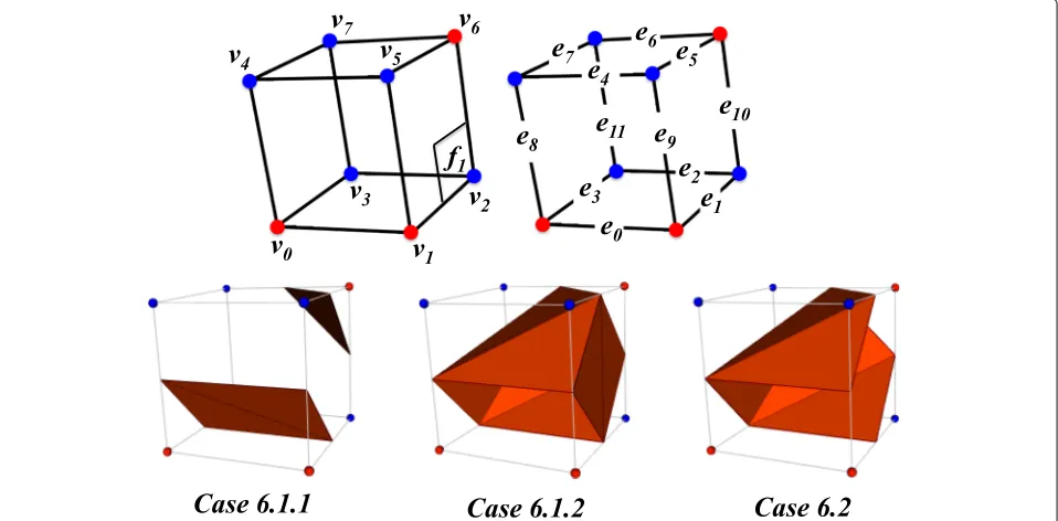
Figure9illustrates the concepts of groups of edges and vertices using the case 6 and its subcases. Red (resp. blue) dots represent positive (resp. negative) scalar values (with respect to the isovalue of interest). The illustrated case 6 is a positive cube with the positive vertices v0, v1, andv6. For each subcase, there are different vertices connectivities that must be respected in the triangulation process.
• Subcase 6.1.1 (bottom left). There is a positive path connecting the verticesv0andv1by the edgee0. The
verticesv0andv1are separated from the vertexv6by
the facef1and the interior of the cube. For this
configurations, there are two groups of vertices
GV0 = {v0,v1}andGV1 = {v6}. And, associated to
them, the groups of edgesGE0 = {e1,e3,e8,e9}and GE1= {e5,e6,e10}.
• Subcase 6.1.2 (bottom middle). The verticesv0andv1
are connected by a positive path by the edgee0. But
related to vertexv6, they are connected by a positive
path only through the interior of the cube and separated from it on the facef1. As the connection is
not given by the facef1, the case 6.1.2 has the same
groups of vertices and edges of the case 6.1.1.
• Subcase 6.2 (bottom right). The verticesv0andv1are
connected by a positive path by the edgee0and
connected to the vertexv6through the interior of the
cube and also by the facef1. In this configuration,
there is only one group of verticesGV0 = {v0,v1,v6}
and, associated to it, the group of edges
GE0= {e1,e3,e8,e9,e5,e6,e10}.
Generating the triangulation
We classify Chernyaev’s lookup table triangulation into three categories:
• Simple leaves , when the isosurface inside the cube is homeomorphic to discs;
• Tunnel, when the isosurface is homeomorphic to a cylinder;
• Interior point, when the isosurface is homeomorphic to a disc and it is necessary to add a point inside the cube for a correct representation.
For each category, we propose a specific triangula-tion process to construct an extended triangulatriangula-tion to the Marching Cubes 33. By using the concept of group of vertices and group of edges, we track the regions defined by the isosurface correctly. The triangulation of the convex hull of a set of point, presented in the Bhaniramka et al. [14] work, is also used to generate the triangulation.
Our method adds, to the topological correctness of Chernyaev’s lookup table, a final mesh free of degenerate triangles. Also, we present in the “Improving the trian-gulation quality of the final mesh” section an application of the proposed method that eliminates the generation of skinny triangles.
The concept ofgroupsproposed in the previous section characterizes the behavior of the trilinear interpolant on the edges and faces of the cube, but not inside it. Observe that, as illustrated in Fig.9, although the cases 6.1.1 and 6.1.2 have different topology of the interpolant, they have the same groups of vertices and edges. If a cube has two or more groups of vertices, they can be separated or joined inside the cube. In order to track the behavior of the trilinear interpolant inside the cube correctly, we use the interior test proposed by Chernyaev [5] and recently improved by Custodio et al. [8].
LetCbe a positive cube and considerGi = GVi
GEi
as the union of the vertices in the group GVi and the
edges in the groupGEi,i = 0, 1,· · ·n−1, wherenis the
number of groups. Let Wi be the set of the intersection
points (by the isosurface) on the edges inGi(for
simplic-ity, let us take the midpoints of the edges inGi; it can be
replaced by the correct position of the point in the genera-tion of the final mesh) and the vertices inGVilabeled with
“=” and “+.”
Once we have checked the vertices connectivity and have used the interior test to classify a given cube into the three categories aforementioned, we construct the triangulation according to the following methods.
Simple leaves triangulation
For each Wi, construct the convex hull conv(Wi). If
it is three-dimensional, then triangulate the boundary
∂(conv(Wi)). Remove from the triangulation the triangles
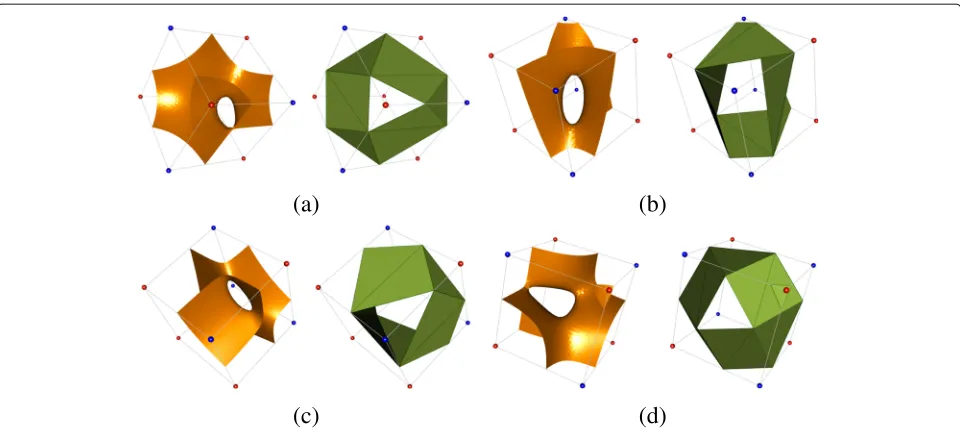
contained on the faces of the cube. The remaining tri-angulation approximates the trilinear interpolant inside the cube (see Fig. 10a). Ifconv(Wi) is contained on the
faces of the cube, return the triangulation of conv(Wi),
except in case where the cube has all its vertices equal to zero. In this case, to avoid duplicate faces, no triangula-tion is generated. In additriangula-tion, to prevent a cube face being triangulated twice into two adjacent cubes, the algorithm tracks the grid faces already triangulated.
Tunnel triangulation
Let W be the set of the middle points of the inter-sected edges. Construct the convex hull conv(W) of W. If it is three-dimensional, then triangulate the boundary
∂(conv(W))and remove from the triangulation the trian-gles which have their three vertices on the same group of edge GEi. The remaining triangulation approximates the
isosurface inside the cube (see Fig.10b).
Interior point leaves triangulation
In this category, the boundary of the isosurface patch is a simple closed polygonal curve, whose vertices are the intersection of the isosurface and cube edges. If all four edges of some face are intersected by the isosurface, the polygonal curve connects pairs of edges based on the behavior of the bilinear interpolant on that face. We cre-ate a triangulcre-ated isosurface patch from this triangulation by adding a vertex in the center of the cube and form-ing triangles from that vertex and the line segments of the polygonal curve.
The triangulation of the case 13
Case 13 is the most complex case in the Chernyaev’s lookup table. In this case, all faces are ambiguous and there are six possibilities for the behavior of the inter-polant. Due to its complexity, to correctly triangulate the subcases 13.3, 13.5.1, and 13.5.2 (see Fig.11), a combina-tion of the proposed triangulacombina-tion methods is necessary. The remaining subcases can be directly triangulated by one of the proposed triangulation methods. Following, we present the combination of the above triangulation methods adopted in our method.
• In case 13.3, there is one group of vertices with four vertices. To triangulate this configuration, we additionally use the negative vertex incident to the three faces on which the positive vertices are joined. We apply the interior point leaves triangulation combined with the simple leaves triangulation in the one negative group with a single vertex as defined above.
(a)
(b)
Fig. 10The triangulation ofasimple leavesandbtunnelcategories in the Marching Cubes 33 triangulation table.aThe top and bottom rows show a configuration with two groups and one group of vertices, respectively.bTunnel triangulation
To triangulate this configuration, we apply the simple leaves triangulation to the two groups of vertices.
• In case 13.5.2, there are two groups of vertices connected by the interior of the cube and a change of the interpolant signal in the region diagonally opposite to the one vertex group. To triangulate this configuration, we apply the tunnel triangulation combined with the simple leaves triangulation in the
region diagonally opposite to the one vertex positive group.
More than the trilinear interpolation
In his work, Chernyaev points out the existence of cases where the behavior of the isosurface could not be covered by the trilinear interpolant. This well-known limitation draws attention to the necessity of the study of other
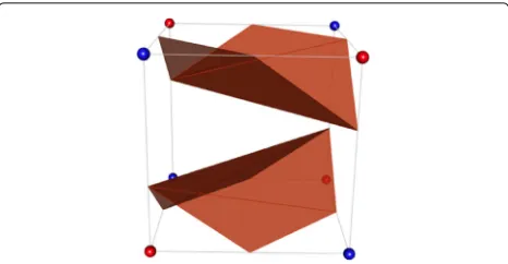
Fig. 12A possible behavior of the isosurface for the signal configuration in case 13 that cannot be covered by the trilinear interpolant
interpolants and, consequently, to the need for methods that are able to construct a discrete approximation to them.
Our triangulation method, based on the connectiv-ity of the cube elements and the region defined by the interpolant inside the cube, represents a first step towards building the triangulation of other interpolants. We emphasized that the triangulation is generated with-out the need of a look up table. Thus, it is enough for a new interpolant to define the regions, and we can gener-ate the triangulation associgener-ated with the isosurface of this interpolant.
In Fig.12, it is shown the possible behavior of the iso-surface, presented by Chernyaev, which cannot be covered
Table 1Comparison of the Betti numbers of the meshes presented in Fig.13, generated by the Raman and Wenger method and our method
B. Numbers Right figure Middle figure Left figure
Correct Our R. W. Correct Our R. W. Correct Our R. W.
b0 1 1 4 1 1 5 1 1 4
b1 0 0 0 2 2 0 2 2 0
b2 1 1 4 1 1 5 1 1 4
by the trilinear interpolant. Observe that, once it is pos-sible to track the connectivity of the cube elements, such triangulation can be constructed by our method.
The topology of the generated mesh
In our method, the concepts of groups of vertices and of edges are introduced to correctly track the behavior of the interpolant on the boundary of the cube.
The Betti numbers are known tools in algebraic topol-ogy to identify and compare topological spaces (Munkres [17]). For surfaces, the Betti number b0 indicates the number of connected components; the Betti number b1 is defined by b1 = 2g, where g is the genus of the surface; andb2 is the number of three-dimensional holes.
In Fig.13, we present meshes extracted from randomly generated trilinear scalar fields, generated by our method and the Raman and Wenger method. In Table1, we show a comparison of the Betti numbers of the generated meshes.
The right example hasb0 = 1 (one connected compo-nent),b1=0 (no genus), andb2=1, so it is equivalent to a sphere. We observe that our algorithm represents cor-rectly the topology, while Raman and Wenger algorithm splits in four components (b0=4).
The middle and the left example has b0 = 1 (one connected component) and b1 = 2 (one genus), so both are equivalent to a torus. Our algorithm repre-sents correctly the topology for both examples, while Raman and Wenger algorithm generates respectively five components (b0 = 5) and four components b0 = 4 without genus.
As noted by Custodio et al. [8] in their work, even when the topology of the trilinear interpolant is tracked correctly, the Marching Cubes 33 may generate non-manifold meshes. In their work, the author observes that the lookup table proposed by Chernyaev can generate non-manifold edges. This occurs when the topology induced by the interpolant inside two adjacent grid cells
(a)
(b)
(c)
(d)
Fig. 15Non-manifold issue caused by the Chernyaev lookup table.aThe zero-level set of a 5×5×5 randomly generated piecewise-trilinear scalar field.bThe mesh generated by our method, in our implementation, was included the solution proposed by Custodio et al. to fix the problem. cThe mesh generated by an implementation of the Marching Cubes 33 algorithm has two non-manifold edges caused by the triangulation proposed by Chernyaev
is homeomorphic to a cylinder, and these cells share an ambiguous face. In these cases, part of the tunnel triangulation on Chernyaev’s lookup table lies on the ambiguous faces (see Fig.14).
Observe that any combination of the configurations shown in Fig. 14, where two adjacent cubes share an ambiguous face, results in the generation of non-manifold edges and in the overlap of the triangulation.
As mentioned by Custodio et al. [8], splitting both grid cells at the critical point (on the face) elimi-nates the ambiguous face shared by two cells. For the sake of simplicity, the author proposed to split all faces in the grid slice that contained the problematic
Fig. 16An example of a grid configuration which will result in a non-manifold triangulation. The blue, red, and yellow grid vertices respectively represent the vertices with the scalar value smaller, greater, and equal scalar value to the isovalue
configuration. In our work, we followed the proposed approach and a grid preprocessing step was added to eliminate configurations as the ones illustrated in Fig. 15, which shows the issues with the Chernyaev’s lookup table and presents the mesh generated by our method.
It is important to note that, once the vertices of the grid can be part of the final triangulation, some con-figurations of the input data can result in non-manifold triangulations. The correct topology, in some cases, implies in the generation of a non-manifold. Figure 16
illustrates one of these possibilities that corresponds to the conic.
Improving the triangulation quality of the final mesh
We now turn to a well-known issue in the Marching Cubes based algorithm, the quality of the resulting mesh. As pre-sented in the “Extended trilinear triangulation” section, our triangulation process naturally avoids the degenerate triangles once; in our method, we consider the possibility of the isovalue match with the scalar field value at a ver-tex of the grid. In this section, we propose a method to eliminate skinny triangle and to improve the aspect ratio of the triangulation. Our main strategy is based on modi-fying the scalar field value on the grid vertices close to an isosurface intersection point.
Fig. 17The meshes generated by the Marching Cubes algorithm from the Bonsai and Aneurysm datasets
histograms presented in Fig.18, in both meshes illustrated in Fig.17, the number of triangles with quality inferior to 0.15, for example, is greater than 10% of the total number of triangles in the meshes.
A strategy commonly used to solve the mesh quality problem is the post processing of the mesh. As presented in the survey Recent advances in remeshing of surfaces proposed by Alliez et al. [18], most of these techniques
are concerned only with the quality of the triangulation, without commitment with the preservation of geometric and, in some cases, topological characteristics of the isosurface.
The main drawback in the cited methods is that the post-processing changes the triangulation without considering if the new mesh corresponds to a representation of the initial isosurface.
0.0 0.1 0.2 0.3 0.4 0.5 0.0 0.1 0.2 0.3 0.4
50000
100000
150000
0
0
5000
10000
15000
20000
25000
q(T) Bonsai dataset
0.5
Fig. 19The topological changes in the generated mesh that are blocked by our optional verification step
On the other hand, techniques that seek to improve the quality of the mesh through modifications made directly in the Marching Cubes algorithm (Dietrich et al. [19,20]) have shown to be effective in improving the quality of the generated mesh while preserving desired charac-teristics of the isosurface. However, these methods are based on the original Marching Cubes look up table, which is unable to represent the behavior of the trilinear interpolant inside the cube correctly.
Also in this direction, Raman and Wenger [10] com-bine their extended triangulation table with the algorithm proposed by Labelle and Shewchuk [21] which, by modi-fication on the scalar field, collapses to the nearest vertex of the grid the intersection points near to it, thus elim-inating the skinny triangles. Nevertheless, as presented in the “The topology of the generated mesh” section, the proposed extended triangulation also has topological issues that are propagated to this application.
The Labelle and Shewchuk [21] algorithm has an input parameter lambda [ 0, 0.5] that given an isovalue alpha, before the extraction of the isosurface, all the intersected edges are detected, and if the intersection point is dis-tant less than λL (L being the length of the edge) from a vertex of grid, then this intersection point is collapsed to the nearest vertex of the grid. To preserve the geom-etry of the mesh, the final step of the algorithm moves each isosurface vertex on a vertex of the grid to the location of the closest isosurface vertex in the original grid.
Seeking to join the Marching Cubes 33 topologi-cal consistency with a better quality of the result-ing mesh, we combine the Labelle and Shewchuk [21] algorithm with our extended triangulation. After pre-processing the grid, we run the Marching Cubes 33 with our extended triangulation and the modified grid. To avoid undesired topological changes in the isosurface
representation caused by the modification of the scalar field values sampled at the vertices of the grid, we add to the method proposed by Labelle and Shewchuk an optional verification step. Given the isovalue and the
λ parameters, we track the isosurface topology changes in the interior of each cube. Once a configuration that could modify the global isosurface topology is detected, this cube and its neighbors are “blocked.” Then, the mesh improvements are performed only in the cubes that are not in the neighborhood of the blocked cubes. In Fig.19, we use the configuration of the lookup table case 4 to illustrate the topological changes blocked in our verification step.
In Fig. 20, we present our result (red) and compare it with the Raman and Wenger [10] work (blue). Although both methods improve the quality of the triangulation (as shown in Fig. 21), our method correctly represents the topology of the trilinear interpolant while the Raman and Wenger [10] method cannot represent the trilin-ear interpolant correctly even when the λ parameter is equal to zero. For λ equal to 0.1, 6.73% of the cubes intersected by the isosurface were blocked in the verifi-cation step and 31.1% of the cubes were blocked for λ equal to 0.2. As illustrated in Fig.22, where we compare the meshes generated by our method forλ equal to 0.2 with and without the verification, the proposed additional step avoided the change of the topology of the generated mesh.
In Fig.23, we present the results obtained by applying the method to remove the skinny triangles of the mesh extracted from the data set Bonsai, with the parameter
Fig. 21Statistics of the quality of the meshes shown in Fig.20
Fig. 23The meshes extracted from the data set Bonsai for the isovalue 39.5, with the parameterλequal to 0.0 (left column) and equal to 0.2 (right column)
meshes shown on the right is superior to the one shown on the left.
In our experiments, we observed that the number of blocked cubes in real datasets is even smaller than the observed in the randomly generated dataset. For the Bonsai dataset, for instance, only 0.63% of the cubes inter-sect by the isosurface was blocked in the verification step, forλequal to 0.2 and the isovalue 39.5.
Conclusion
We have presented a new method to generate an extended triangulation to the Marching Cubes 33 algorithm, which guarantees a correct interpretation of the trilinear interpolant.
We have compared our result with a related method and pointed out the existence of topological issues in the mesh generated by it.
In addition, we applied our extended triangulation pro-cess to improve the quality of the triangulation in the resulting mesh, a well-known issue on meshes generated by algorithms based on Marching Cubes.
For future work, we plan to use the cube connectivity concepts to study the behavior of others interpolants in the Marching Cubes algorithm. We also plan to generalize the extended triangulation with the intent of obtain-ing a topologically correct Marchobtain-ing Cubes in higher dimensions.
0.0 0.1 0.2 0.3 0.4 0.5 0.0 0.1 0.2 0.3 0.4 0.5
50000
100000
150000
0
q(T): Bonsai dataset = 0.0 q(T): Bonsai dataset = 0.2
200000
250000
50000
100000
150000
0
200000
Acknowledgements
The authors wish to thank Tiago Etiene for his valuable help with the paper. The datasets used in this work can be download from the Volvis project web page (https://labs.cs.sunysb.edu/labs/vislab/volvis/).
Funding
This research received no specific grand from any agency in the public, commercial, or not-for-profit sectors.
Availability data and materials
The results of this paper are reproducible. Information on the executable figures in this paper and the randomly generated datasets can be accessed and downloaded from the project page (https://liscustodio.github.io/
ExtendedMC33/).
Authors’ contributions
LC developed the theoretical formalism, performed the analytic calculations, and took the lead in writing the manuscript. SP and CS discussed the results, provided critical feedback, and helped shape the research, analysis, and manuscript. All authors read and approved the final manuscript.
Competing interests
The authors declare that they have no competing interests.
Publisher’s Note
Springer Nature remains neutral with regard to jurisdictional claims in published maps and institutional affiliations.
Author details
1Computational Modeling Department, Polytechnic Institute at the Rio de
Janeiro State University, Rio de Janeiro, Brazil.2Department of Mathematics,
Pontificial Catholic University of Rio de Janeiro, Rio de Janeiro, Brazil.
3Computer Science and Engineering Department, New York University, New
York City, USA.
Received: 26 January 2018 Accepted: 28 January 2019
References
1. Lorensen WE, Cline HE (1987) Marching Cubes: a high resolution 3D surface construction algorithm. SIGGRAPH Comput Graph 21:163–169 2. Dürst M (1988) Letters: additional reference to marching cubes. Comput
Graph 22(2):72–73
3. Nielson GM, Hamann B (1991) The asymptotic decider: resolving the ambiguity in marching cubes. In: Proceedings of the 2nd Conference on Visualization. IEEE Computer Society Press, Los Alamitos. pp 83–91 4. Natarajan BK (1994) On generating topologically consistent isosurfaces
from uniform samples. Vis Comput 11(1):52–62.https://doi.org/10.1007/ BF01900699
5. Chernyaev EV (1995) Marching Cubes 33: construction of topologically correct isosurfaces. Technical Report CN/95-17, Institute for High Energy Physics
6. Nielson GM (2003) On marching cubes. IEEE Trans Vis Comput Graph 9:283–297.https://doi.org/10.1109/TVCG.2003.1207437
7. Lewiner T, Lopes H, Vieira AW, Tavares G (2003) Efficient implementation of Marching Cubes’ cases with topological guarantees. J Graph Tools 8(2):1–15
8. Custodio L, Etiene T, Pesco S, Silva C (2013) Practical considerations on marching cubes 33 topological correctness. Comput Graph 37(7):840–850.https://doi.org/10.1016/j.cag.2013.04.004 9. Grosso R (2016) Construction of topologically correct and manifold
isosurfaces. Comput Graph Forum 35(5):187–196.https://doi.org/10. 1111/cgf.12975
10. Raman S, Wenger R (2008) Quality isosurface mesh generation using an extended marching cubes lookup table. Comput Graph Forum 27:791–798
11. Montani C, Scateni R, Scopigno R (1994) A modified look-up table for implicit disambiguation of marching cubes. Vis Comput 10(6):353–355 12. Lachaud J-O, Montanvert A (2000) Continuous analogs of digital
boundaries: a topological approach to iso-surfaces. Graph Model 62(3):129–164.https://doi.org/10.1006/gmod.2000.0522
13. Bhaniramka P, Wenger R, Crawfis R (2000) Isosurfacing in higher dimensions. In: Proceedings of IEEE Visualization 2000, Ertl, Hamann, Varshney, Ed. IEEE Visualization Proceedings. pp 15–22
14. Bhaniramka P, Wenger R, Crawfis R (2004) Isosurface construction in any dimension using convex hulls. IEEE Trans Vis Comput Graph 10(2):130–141 15. Wang X, Niu Y, Tan L-W, Zhang S-X (2014) Improved marching cubes
using novel adjacent lookup table and random sampling for medical object-specific 3D visualization. J Softw 9(10):2528–2537
16. Cirne MVM, Pedrini H (2013) Marching cubes technique for volumetric visualization accelerated with graphics processing units. J Braz Comput Soc 19(3):223–233.https://doi.org/10.1007/s13173-012-0097-z 17. Munkres JR (1993) Elements of algebraic topology. Addison-Wesley,
Boston
18. Alliez P, Ucelli G, Gotsman C, Attene M (2008) Recent advances in remeshing of surfaces. In: Shape Analysis and Structuring, Mathematics and Visualization. Springer-Verlag, Berlin
19. Dietrich CA, Scheidegger CE, Comba J, Dihl L, Nedel LP, Silva CT (2009) Marching cubes without skinny triangles. Comput Sci Eng 11(2):82–87 20. Dietrich CA, Scheidegger CE, Schreiner JM, Comba J, Dihl L, Nedel LP, Silva CT
(2009) Edge transformations for improving mesh quality of marching cubes. IEEE Trans Vis Comput Graph 15(1):150–159