International Journal of Terrestrial Heat Flow and Applied Geothermics
VOL. 1, NO. 1 (2018); P. 6-13. ISSN: 2595-4180
DOI:https://doi.org/10.31214/ijthfa.v1i1.6 http://ijthfa.com/
6
Keywords
Global Heat Flow, Digital Maps, GIS Techniques,
Received: January 28, 2018 Accepted: April 18, 2018
Published: April 26, 2018
Global Heat Flow: New Estimates Using Digital
Maps and GIS Techniques
Fábio Vieira1, Valiya Hamza1
1Observatório Nacional, Rio de Janeiro, Brazil.
Email address
[email protected] (V. Hamza) Corresponding author
Abstract
The digital geophysical maps and GIS (Geographic Information System) techniques have been employed in obtaining a better understanding of global heat flow. The starting point has been a system of 1o x 1o equal longitude grid consisting of 64800 cells. Superposed on
this grid system are a set of 190 polygons that approximates boundaries of tectonic provinces and another set of 137 polygons that outlines age provinces. The area extents of these “tectonic polygons” were determined, and heat flow values calculated based on the empirical relation between heat flow and age of last thermos-tectonic event. Maps derived using such polygon representations reveal a pattern quite similar to that obtained in higher-degree spherical harmonic representations of global heat flow. In addition, an updated assessment of observational data has been carried out and estimated values assigned for cells where observational data are currently unavailable. This practice has been found to provide reasonable bounds in interpolations, leading to better representations of heat flow on a global scale. The mean global heat flow values obtained by this procedure is found to fall in the interval of 58 to 63mW/m². This estimate is lower than that reported in some of the previous studies in which use has been made of theoretical values derived from half-space cooling models as substitutes for experimental data. According to the results of the present work, based on reappraisal of global heat flow database and with due emphasis on observational data, the global conductive heat loss falls in the range of 28 to 35TW. This is nearly 22 to 35% less than those reported in earlier studies.
1. Introduction
Measurements of terrestrial heat flow in boreholes penetrating the near surface layers provide valuable information on the internal thermal field of the Earth and estimates of global heat loss. The problem however is that availability of experimental data is not available for all regions, there being large areas without suitable data. One of the ways of getting around this problem is to employ empirical relations between heat flow and geological characteristics of near surface layers. Preliminary indications of a correlation between heat flow and geologic age was pointed out by Hamza (1967). Following this, empirical relations between heat flow and tectonic age were proposed (Polyak and Smirnov, 1968; Hamza and Verma, 1969). In a later work (Chapman and Pollack, 1975) derived maps of global heat flow where the empirical relation with age was employed in estimating heat flow values for areas for which experimental data were not available. In the procedure adopted by Chapman and Pollack (1975) the heat flow estimates were made on the basis of dominant geological features identifiable in 5o x 5o equal
longitude cells. A similar procedure was adopted by Pollack et al (1993) in deriving improved global heat flow maps
where the referencing system for tectonic age was based on a grid of 1o x 1o equal longitude cells. However. selection of
dominant geology in each cell and estimation of number of cells were manual and prone to potential errors. More importantly, Pollack et al (1993) employed theoretical heat flow values, derived from half-space cooling model, as substitutes of observational data for regions of oceanic crust with ages less than 55 Ma. Validity of this approach was questioned by Hamza et al (2008a). In the later works of Davies and Davies (2010) and Vieira et al (2010) it was pointed out that the adverse effects of some of these problems may be minimized by adopting the use of modern techniques of handling geospatial data.
model for ocean regions with ages less than 55 Ma. In the present work, it is argued that values derived from half-space cooling models lead to overestimation heat flow for young ocean crust.
2. Digital Maps and GIS Techniques
Availability of digital thematic maps based on techniques of geographic information system (GIS) has opened up the possibility of assigning theoretical heat flow values, with improved accuracy. This technique also allows appropriate weighting for the tectonic context and is particularly suitable for elaboration of digital geological and geophysical maps and in handling irregularly spaced data sets. The digital maps of 1o x 1o cells for continental and oceanic regions, adapted from
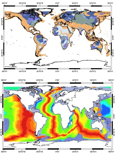
Mooney et al (1998) and Muller et al (1997), are illustrated in Figure 1.
Figure 1 - Digital maps of tectonic units employed in obtaining estimates of terrestrial heat flow. The top panel refers to digital map of tectonic provinces in continental regions. The bottom panel refers to digital isochrone map for oceanic regions (Adapted from Hamza
and Vieira, 2010).
Global geophysical maps of tectonic provinces presented by Mooney et al (1998) cover platforms, shields, large igneous provinces, basins, orogens and areas of extended crust. Also provided in this reference are global maps of last thermos-tectonic events for the geologic periods of Arquean, Proterozoic (early, middle and late periods), Paleozoic and Meso-Cenozoic. Digital isochrone maps by Muller et al (1997) allow identification of age provinces in oceanic regions. In the present work, we make use of digitized versions of these maps in investigating the nature of terrestrial heat flow variations on global scale.
In the work of Vieira et al (2010) the procedure adopted in handling digital maps consists of outlining tectonic units over 1o x1o equal longitude grids. Such a grid system consists of
64800 cells. Of these 22.380 cells cover the continental crust and 42.420 cells cover the oceanic crust. The changes relative to the data set reported by Vieira et al (2010) include incorporation of improved data sets for the South American continent. In particular, there has been significant improvement in the number of heat flow values in Colombia (reported in INGEOMINAS, 2009) and recent new data for central and northern regions (Vieira, 2010) of Brazil.
According to the updated data sets 44386 grid elements have one or more observational data. Estimated heat flow values were employed for the remaining 54769 grid elements. Six categories of tectonic age were used in outlining the polygons. A set of 137 polygons was found sufficient in delimiting the tectonic age pattern for continental areas. In the case oceanic areas 15 categories of tectonic age were used in outlining the polygons. A set of 13 polygons was found sufficient in delimiting the tectonic age pattern. Superposed on this grid system are a set of 190 polygons that delimit the boundaries of tectonic provinces and another set of 137 polygons that delimit the tectonic age pattern.
3. Estimates of Heat Flow for Polygons
Following the practice adopted by Mooney et al (1998) the tectonic age provinces considered in calculations of estimated heat flow values in continental areas are Arquean, Paleo Proterozoic, Meso-Proterozoic, Neo-Proterozoic, Paleozoic and Meso-Cenozoic. Updated data sets were employed in calculating mean values of heat flow for these provinces lying in the continents of North America, South America, Europe, Africa, Asia and Australia. Table 1 provides a summary of the results obtained. It reveals a general trend of decreasing heat flow with age. Thus, relatively high heat flow values were found for younger provinces of Cenozoic and Mesozoic ages, compared with those of older ones with Proterozoic and Arquean ages. For example, heat flow in excess of 80mW/m2
occur in all continental age provinces of Meso-Cenozoic times. On the other hand, all Arquean shields have heat flow less than 50mW/m2.
Table 1 - Summary of mean heat flow values assigned for tectonic polygons in continental regions. The abbreviations used are: NA – North America; SA – south America; EU – Europe; AF – Africa; AS
– Asia; AU – Australia.
Tectonic Age Heat Flow (mW/m
2)
NA SA EU AF AS AU
Cenozoic 120 81 78 82 88 100 Mesozoic 75 64 72 81 63 80 Paleozoic 52 46 47 64 54 79 Neo Proterozoic 48 74 43 65 63 83 Paleo Proterozoic 46 64 44 53 59 61 Arquean Shields 50 45 42 49 46 40
general a general trend of decreasing heat flow with age of ocean floor is observed. Thus, heat flow in excess of 80mW/m2 are found in young ocean crust with ages less than
20Ma.
Table 2 - Summary of mean heat flow values assigned for tectonic polygons in oceanic regions (adapted from Pollack et al, 1993).
Age Interval (Ma) Heat Flow (mW/m²)
Lower Upper
0 11 132
11 20 88
20 33 74
33 40 66
40 48 63
48 68 58
68 83 54
83 127 49
127 132 47
132 140 46
140 148 45
148 154 45
154 180 44
In determining heat flow variations on the basis of polygons of age provinces it is convenient to make use of an equation that accounts for the nature of the empirical relation. In the present context, a relation that allows for variation of heat flow with inverse square root of age seems appropriate. Such an equation may be written as:
𝑞(𝑡) = 𝑐 ∗ )*
√,+ 𝛽/ (1)
where q(t) is the heat flux at time t, c is a scaling constant and a and b are terms employed in numerical approximation. The parameter a is related to the “degree of influence” of thermo-tectonic event on the crustal layers. Thus, the product C*a has an inverse relation with heat flow. The parameter b
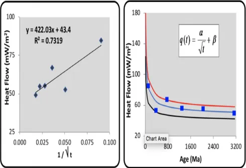
may be considered as representative of heat flow in old crust, where thermal contributions of older tectonic events are relatively insignificant at present times. The variation of heat flow with age for continental regions, derived from data reported in Polyak and Smirnov (1968), Hamza and Verma (1969) and Pollack et al (1993), is illustrated in Figure 2.
In this figure the left panel illustrates the variation heat flow with the inverse square root of age. The right panel indicates variation heat flow as a function of age for three different values of the product c*a. The fit indicated by the blue curve has the value of 422 for the product C*a. This value is in reasonable agreement with that proposed by Hamza (1979). The red and black curves may be considered as indicative of upper and lower bounds that bracket the observational trends. A summary of the parameters employed the fits is provided in Table 3.
Figure 2 - Relations between heat flow (q) and age (t) for continental regions (left and right panels). The red and black curves
indicate upper and lower bounds.
Table 3 - Parameters of equation 1 for continental regions.
FIT C a b
Mean 1 422 43
Upper Bound 1.4 350 35
Lower Bound 0.9 300 42
The variation of heat flow with age for oceanic regions is illustrated in Figure 3. As in the case of continental regions discussed above, the left panel illustrates the variation heat flow with the inverse square root of age while the right panel indicates variation heat flow as a function of age for three different values of the product c*a. The fit is indicated by the blue curve refer to a value of 120 for the product C*a. The red curve, for which the value of the product C*a is 192, may be considered as the upper bound. The black curve for which the value of the product C*a is 72 may be considered as the lower bound. A summary of the parameters employed in such fits is provided in Table 4.
Figure 3 - Relations between heat flow (q) and age (t) for oceanic regions (left and right panels). The red and black curves indicate
upper and lower bounds.
Table 4 - Parameters of equation -1 for oceanic regions.
FIT C a b
Selected 1 120 45
Upper Bound 1.2 160 35
3. Global Map of Cell-Averaged Values
The map of global heat flow derived on the basis of cell-averaged values, with weighting for the tectonic context, is illustrated in Figure 4. Note that assigning cell averaged values of heat flow for the tectonic polygons have led to considerable improvements in outlining boundaries of associated heat flow anomalies Vieira and Hamza (2011). For example, most of the regions with high heat flow anomalies (with values higher than 60mW/m2) are associated with lithospheric plate boundaries,
while most of the ocean basins and interior parts of continental regions are characterized by heat flow less than 60mW/m2.
Also, the widths of high heat flow anomalies associated with mid-ocean ridge areas are narrower.
Figure 4 - Global representation of estimated heat flow values (in units of mW/m2), based on digital maps and empirical relation with
age (Modified after Vieira and Hamza, 2011; Hamza, 2013).
5.
Global map of Observational Data
The global heat flow database in its present form is an outgrowth of earlier compilations (e.g. Birch, 1954; Lee, 1963; Lee and Uyeda, 1965; Jessop et al, 1976; Chapman and Pollack, 1975; Pollack et al, 1993; Hamza et al, 2008a). In the present case, we have used an updated data set of surface heat flow that includes information available in the original compilation of the International Heat Flow Commission - IHFC, additional values reported in the recent study of Davies and Davies (2010) as well as updated values for the South American continent (Vieira and Hamza, 2011). In the earlier works (Pollack et al, 1993; Davies and Davies, 2010) heat flow values assigned to cells located in areas of young ocean crust have been derived on the basis of the half-space cooling – HSC model of Stein and Stein (1992). In later works Vieira and Hamza (2011), Hamza (2013) and Cardoso and Hamza (2011) use was made of values derived from the Finite Half-Space – FHS model. A summary of data sets, employed in deriving global heat flow maps is provided in Table 5.
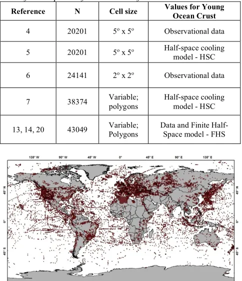
The total number of heat flow values in the updated data set is 44386. The locations of heat flow measurements of the updated data sets are illustrated in the map of Figure 5.
Note that there are significant variations in data density. Antarctica, Greenland and central parts of Africa and South America remain as regions of low data density. This data set has been employed in calculating mean values for a global grid system composed of 1o x 1o equal longitude cells. In spite of
recent advances in in experimental works the number of cells for which observational data are unavailable is nearly 20%. This poses a serious problem in deriving global maps based exclusively on observational data. In such cases, it is clear that
some type of interpolation scheme is necessary in assigning “representative” values to empty cells.
Table 5 - Summary of data sets employed in deriving global heat flow maps. N refer to number of Observational data.
Reference N Cell size Values for Young Ocean Crust
4 20201 5o x 5o Observational data
5 20201 5o x 5o Half-space cooling
model - HSC
6 24141 2o x 2o Observational data
7 38374 Variable; polygons Half-space cooling model - HSC
13, 14, 20 43049 Variable; Polygons Data and Finite Half-Space model - FHS
Figure 5 - Locations of heat flow measurements as per the updated global heat flow data set (Modified after (Vieira and Hamza, 2011;
Hamza, 2013).
It is convenient to note in this context that the availability of estimated heat flow with appropriate weighting for the tectonic setting has opened up the possibility of assigning representative values of heat flow for cells for which observational data are currently not available. This in practice amounts to use of a mixed data set consisting mostly of bin averaged values derived from observational data along with a small set of suitably selected estimated values. A geographic distribution of integrated data sets (observational data and estimated values) is illustrated in figure 6. Here a 50 x 50 mesh
system was used for a representation of the data sets. In this figure cells with the experimental data are indicated in red color and cells with estimated heat flow values in white.
Figure 6 - Illustration of cell averaged data distribution based on a 50x50 mesh system. The background color for continental areas is
It must however be noted that heat flow values assigned to cells located in areas of young ocean crust have been derived on the basis of FHS model. The cell-averaged heat flow values are in the range of 30 - 150mW/m2. The mean heat flow for
cells in the continental regions is 58 +/- 10mW/m2, which is
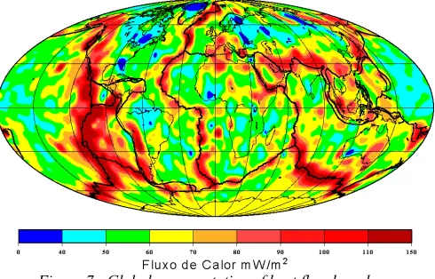
not significantly different from that for cells in the oceanic regions. The global heat flow map derived on the basis of such a mixed data set is presented in Figure 7.
Figure 7 - Global representation of heat flow based on observational data, supplemented with estimates derived from digital maps and empirical correlation with age (Modified after
Vieira and Hamza, 2011; Hamza, 2013).
It is readily apparent that the large-scale features present in this map are quite similar to those of the theoretical heat flow map of Figure 5. Thus. the divergent plate boundary regions (such as the Nazca plate in the Pacific. areas off the west coast of the United States. the Sea of Japan and the Red Sea) stands out as oceanic regions of relatively high heat flow (>80 mW/m2). Also, mid-ocean ridges in the Atlantic. Pacific and
Indian oceans also appear as areas of high heat flow (typically in the range 90-150 mW/m2). The ocean basins and areas of
low angle subduction appear to be characterized by normal heat flow (in the range 50-70 mW/m2). On the contrary. the
central parts of the continental areas of Africa. Asia. North America. South America. Antarctica and Australia seem to be characterized by relatively low heat flow (<60 mW/m2).
6. Discussion
The discussion here is focused on the differences between heat flow maps of the present work and those of previous ones. As mentioned earlier, most of the differences originate from the use of model values employed in deriving estimates of heat flow values for young ocean crust. The previous works (Pollack et al, 1993; Davies and Davies, 2010) rely heavily on the use of half-space cooling (HSC) and Plate models in deriving estimated values. However, these models are known to be largely incompatible with observational data reported in Parsons and Sclater (1977) and Sclater et al (1980). A comparative analysis of the lithosphere models and procedures used in calculating heat flow values are provided in the following sections. This is followed a brief discussion of implications for global heat loss.
6.1. Lithosphere Model considerations
In the Half-Space Cooling (HSC) model the lithosphere is considered as the boundary layer of mantle convection cells.
The lithosphere grows in thickness continuously as it moves away from the up-welling limb of the mantle convection system. The cooling process of the lithosphere is assumed to be conductive and one-dimensional. The fit of HSC model curve to observational heat flow data is known to be poor (e.g. Hofmeister and Criss, 2005; 2006; 2008). It overestimates heat flow in ocean crust with ages less than 60 Ma and underestimates heat flow for crust with ages greater than 100 Ma (Parsons and Sclater, 1977; Sclater et al, 1980). Such difficulties arise from the implicit assumption of the HSC model that the wavelength of the problem domain is unbounded (Cardoso and Hamza, 2011). It implies that the thickness of the material undergoing solidification beneath the boundary layer is large compared to the stable thickness of the lithosphere at large distances from the ridge axis (Cardoso and Hamza, 2011). As pointed out by Hamza et al (2008) and Vieira et al (2010) this condition cannot be considered as satisfactory for the physical domain of the problem under consideration, since the upwelling material beneath the ridge axis has a finite width. Since this is the same magmatic material that moves laterally away from the ridge zone, its thickness has to be finite (Hamza, 2013).
The Plate model proposed by McKenzie (1967) is known to provide a better fit to heat flow data from ocean crust with ages greater than 100 Ma. Nevertheless, it also overestimates heat flow for ocean crust with ages less than 55 Ma. In an attempt to overcome such difficulties Stein and Stein (1992) proposed a hybrid version, referred to also as the Global Depth Heat Flow (GDH) reference model. The GDH model is successful in providing a satisfactory explanation for regional variations in bathymetry but fail in accounting for the low values of heat flow in ocean crust with ages less than 55 Ma. The problem eventually came to be known as the oceanic heat flow paradox. It was in this context that Stein and Stein (1992) and Pollack et al (1993) invoked the hypothesis of regional scale hydrothermal circulation in ocean crust as a possible mechanism responsible for the appearance of this paradox. Nevertheless, the proposed scheme of water circulation is based on the highly unreasonable assumption that lateral flow of cold water occurs over large distances through impermeable oceanic crust, from areas of stable segments away from spreading zones to areas near the ridge axis. Available evidences on hydrothermal circulation in ocean floor (see for example: Williams et al, 1974; Haymon et al, 1991; German et al, 1994) indicate that such processes are limited to narrow belts in the vicinity of spreading centers. There are no evidences for large scale subsurface flows in stable ocean crust. In addition, it seems unlikely that fluid pressure heads needed for driving such flows can be generated by differences in lateral temperatures.
does not address explicitly the thermal effects of latent heat at the lithosphere – asthenosphere boundary.
It was in this context that Cardoso and Hamza (2011) and Hamza (2013) proposed a new approach that incorporates the effects of latent heat and buffered solidification and at the same time provide a satisfactory solution for large scale variations of bathymetry and heat flux in the ocean floor. Designated as the Finite Half Space model - FHS, it introduces the assumption that the wavelength of the solution of the relevant heat conduction equation is related to the thickness of the stable lithosphere at large distances from the ridge axis. A major consequence of this assumption is that it imposes an asymptotic limit for the vertical growth of the lithosphere at the expense of the asthenosphere. Under these conditions the solution for the temperature (T) at depth (z) in the oceanic lithosphere of age (t) and of basal temperature (Tm) is (Cardoso and Hamza, 2011; Hamza, 2013):
(2)
where a is the asymptotic value for the thickness of the lithosphere in stable ocean basins and kmod is the modified thermal diffusivity, that takes into account the role of latent heat. A brief description of the theoretical basis of the FHS model and its application to heat flow is presented in the Appendix.
The relations for surface heat flux and bathymetry within the framework of the FHS model were also derived by Cardoso and Hamza (2011) and Hamza (2013). For the case of constant thermal diffusivity, the equation for surface heat flux in FHS model may be written as:
(3)
A comparative illustration of the half-space and plate model fits is illustrated in figure 8. Note that FHS model provides a far better fit to experimental data than those found for other model fits.
A careful examination of Eq. (3) reveals that the solution provided by the FHS model represents the general case for thermal models of the lithosphere. In fact, it is possible to demonstrate that the solutions derived in the HSC and Plate models represent particular end member cases of the FHS model. Consider for example the solution (3) for small values of time and values of depth much less than the thickness of the stable lithosphere. In this case the right-hand side of Eq. (3) is nearly identical to that of the fundamental solution for temperature in the HSC model, the only difference being the modified form of thermal diffusivity. On the other hand, for depth values nearly equal to the stable thickness of the lithosphere the right-hand side of Eq. (1) approaches unity, which is the limiting condition employed in the Plate model of McKenzie (1967). In other words, the FHS model behavior is similar to that of the HSC model for small times but similar to that of the Plate model for large times.
Figure 8 - Comparison of fits to observational oceanic heat flow data. Note that the fit for finite half-space model (FHS) is far superior when compared with those of HSC and GDH models
(Adapted from Hamza, 2013).
6.2. Global Heat Loss
A topic of related interest is the problem of Global Heat Loss. Pollack et al (1993) reported a value of 44.2+/- 1.0 terawatt (TW) for global heat loss, which has found wide acceptance in the current literature. Similar estimates were also reported in the recent work of Davies and Davies (2010). In such estimates extensive use has been made of theoretical heat flow values, derived from the HSC model, in estimating heat losses for areas of young ocean crust. The justification for this practice (of using theoretical values as substitute for experimental data) is based on the argument that measured heat flow values in areas of young ocean crust are affected by the perturbing effects of hydrothermal circulation and hence not representative of total heat flux. However, the role of heat transport by hydrothermal circulation in young ocean crust and its influence on global heat loss has been examined in detail in a number of recent works (see for example: Hofmeister and Criss, 2005; 2006; 2008; Hamza et al, 2008b; Vieira et al, 2010). The main conclusion emerging from these studies is that hydrothermal circulation operates on local scales at or near the ridge axis. However, it is not an effective mechanism for heat transport on regional scales. In fact, as pointed out recently, the hypothesis of regional hydrothermal circulation (which assumes inflow of cold water in high heat flow areas and outflow of hot water in low heat flow areas) contradicts the very basic principles of thermal convection. According to the results of the present work, based on reappraisal of global heat flow database and with due emphasis on observational data, the global conductive heat loss falls in the range of 28 to 35TW. This is nearly 22 to 35% less than those reported in earlier studies.
7. Conclusions
In the present work digital geophysical maps and GIS techniques have been employed in delimiting spatial domains of tectonic provinces and age patterns and in obtaining better understanding of global heat flow. A system of 1o x 1o equal
longitude grid consisting of 64800 cells was employed for this purpose. Superposed on this grid system are a set of 190 polygons that approximates boundaries of tectonic provinces and another set of 137 polygons that outlines age provinces. The area extents of these polygons were determined, and heat flow values calculated for this set of “tectonic polygons” based
(
)
(
(
)
)
t
a
erf
t
z
erf
T
T
T
t
z
T
mmod mod 0
0
2
2
)
,
(
k
k
-+
=
(
t
)
erf
(
a
t
)
T
T
t
q
mz
mod mod
0 0
2
1
)
(
)
(
k
k
p
l
on the empirical relation between heat flow and age of last thermos-tectonic event. Maps derived using such polygon representations reveal a pattern quite similar to those obtained in higher-degree spherical harmonic representations of global heat flow. In addition, an updated assessment of observational data has been carried out and estimated values assigned for cells for which observational data are currently unavailable. The mean global heat flow values obtained by this procedure is found to fall in the interval of 58 to 63mW/m2.
The abovementioned range of values is lower than that reported in some of the previous studies in which use has been made of theoretical values derived from half-space cooling models as substitutes for experimental data. Finite half-space model is found to provide better estimates of heat flow for all age ranges of ocean crust, there being no need to invoke the hypothesis of regional hydrothermal circulation in ocean crust with ages greater than 20Ma.
According to the results of the present work, based on reappraisal of global heat flow database and with due emphasis on observational data, the global conductive heat loss falls in the range of 28 to 35TW. This is nearly 22 to 35% less than those reported in earlier studies.
8. Acknowledgment
This work was carried out as part of M.Sc. Thesis work of the first author. The second author is recipient of a research scholarship (Process No. 306755/2017-3) granted by Brazilian National Research Council - CNPq. We thank Dr. Papa for institutional support.
References
Birch, F. 1954. The Present State of Geothermal Investigation, Geophysics, 19, 645-659.
Cardoso, R.R., Hamza, V.M. (2011). Finite Half pace model of oceanic lithosphere. In: ‘Horizons in Earth Science Research’, Benjamin Veress and Jozsi Szigethy, (Editors), v.5, 151-162, ISBN 978161209X, Nova Science Publishers Incorporated.
Cardoso, R.R., Ponte Neto, C.F.; Hamza, V.M. 2005. A reappraisal of global heat flow data. Proceedings. 9th International Congress of the Brazilian Geophysical Society. Salvador. Brazil. 6 pages.
Chapman D.S., Pollack H.N. 1975. Global heat flow: a new look. Earth Planet Sci Lett., 28, 23–32.
Davies. J.H., Davies D.R. 2010. Earth´s surface heat flux. Solid Earth. Vol. 1. p. 5-24.
German, C.R., Briem, J., Chin, C., Danielsen, M., Holland, S., James, R., Jonsdottir, A, Ludford, E., Moser, C., Olafson, J., Palmer, M.R., Rudinicki, M.D. 1994. Hydrothermal activity on the Reykjanes Ridge: the Steinaho ll Vent-field at 63_060N. Earth Planet Sci Lett 121:647–654.
Giambalvo, E.R., Fisher, A.T., Martin, J.T., Darty, L., Lowell, R.P. 2000. Origin of elevated sediment permeability in a hydrothermal seepage zone. eastern flank of the Juan de Fuca Ridge. and implications for transport of fluid and heat. J. Geophys. Res 105:913–928.
Hamza. V.M. 1967. The relationship of heat flow with geologic age. Internal Report. National Geophysical Res. Institute. Hyderabad (India).
Hamza, V.M. 1979. Variation of continental mantle heat flow with age: Possibility of discriminating between thermal models of the lithosphere, Pure and Applied Geophysics, vol. 117, pp. 65 - 74.
Hamza, V.M. 2013. Global Heat Flow without invoking ‘Kelvin Paradox’, Frontiers in Geosciences, Volume 1, No.1, PP. 11-20.
Hamza, V.M., Cardoso, R.R., Alexandrino, C.H. 2010. A magma accretion model for the formation of oceanic lithosphere: Implications for global heat loss, International Journal of Geophysics, pp. 1-16.
Hamza V.M., Cardoso R.R., Ponte Neto C.F. 2008a. Spherical Harmonic Analysis of Earth's Conductive Heat Flow. International Journal of Earth Sciences, 97, 205-226. Hamza V.M., Cardoso R.R., Ponte Neto C.F. 2008b. Reply to
comments by Henry N. Pollack and David S. Chapman on ‘‘Spherical harmonic analysis of Earth’s conductive heat flow’’. International Journal of Earth Sciences, 97, 233-239.
Hamza, V.M., Verma, R.K. 1969. Relationship of heat flow with the age of basement rocks, Bull. Volcan., 33, 123-152.
Haymon, R.M., Fornari, D.J., Edwards, M.H., Carbotte, S., Wright, D., Macdonald, K.C. 1991. Hydrothermal vent distribution along the East Pacific Rise crest (9o09’– 54’ N) and its relationship to magmatic and tectonic processes on fast-spreading mid-ocean ridges. Earth Planet. Sci. Lett., 104:513-534.
Hofmeister, A.M., Criss, R.E. 2005. Earth’s heat flux revised and linked to chemistry, Tectonophysics, vol. 395, pp. 159-177.
Hofmeister, A.M.; Criss, R.E. 2006. Comment on “Estimates of heat flow from Cenozoic sea floor using global depth and age data”, by M. Wei and D. Sandwell”, Tectonophysics, vol. 428, pp. 95-100.
Hofmeister, A.M., Criss, R.E. 2008. Model or measurements? A discussion of the key issue in Chapman and Pollack’s critique of Hamza et al.’s re-evaluation of oceanic heat flux and the global power, International Journal of Earth Sciences, vol. 97, pp. 239-243.
INGEOMINAS. 2009. Mapa geotérmico de Colombia, Instituto De Investigación E Información Geocientífica, Minero Ambiental Y Nuclear, Exploración Y Evaluación De Recursos Geotérmicos. República De Colombia, Ministerio De Minas Y Energía, Bogotá, Colombia.
Jessop, A. M., Hobart, M. A., Sclater, J. G. 1976. The World Heat Flow Data Collection – 1975, Geothermal Series 5, Earth Phys. Branch, Ottawa, 125 p.
Lee W.H.K. 1963. Heat flow data analysis. Reviews of Geophysics. 1:449–479.
Lee W.H.K., Uyeda S. 1965. Review of heat flow data. In: Lee W.H.K (Eds) Terrestrial heat flow. Geophysical monograph series 8. AGU. Washington. pp 87–100. McKenzie, D.P. 1967. Some remarks on heat flow and gravity
anomalies. J. Geophys. Res., 72, 6261 – 6273.
Mooney. W.D., Laske, G., Masters T.G. 1998. CRUST 5.1: A global crustal model at 5° × 5°. J. Geophys. Res. V. 103. No. B1. 727–747. 1998.
Parsons, B., Sclater, J. G. 1977. An analysis of the variation of ocean floor bathymetry and heat flow with age, J. Geophysics. Res., 82, 803-827.
Pollack H.N., Hurter S.J., Johnson J.R. 1993. Heat flow from the earth’s interior: analysis of the global data set. Rev. Geophys., 31, 267–280.
Polyak B.G., Smirnov Y.A. 1968. Relationship between terrestrial heat flow and tectonics of continents. Geotectonics, 4, 205–213 (Eng. Transl.).
Sclater, J.G, Jaupart, C, Galson, D. 1980. The heat flow through oceanic and continental crust and heat loss of the Earth. Rev Geophys. 18:269–311.
Stein, C., Stein, S. 1992. A model for the global variation in oceanic depth and heat flow with lithospheric age. Nature 359:123–129.
Vieira, F.P., Cardoso, R.R., Hamza, V.M. 2010. Global Heat Loss: New Estimates Using Digital Geophysical Maps and GIS Techniques. Proceedings of the IV Brazilian Symposium on Geophysics, 14 - 17 November, Brasília.
Vieira, F.P., Hamza, V.M. 2011. Global Heat Flow: Comparative analysis based on experimental data and theoretical values. Proceedings of Twelfth International Congress of the Brazilian Geophysical Society, 1-6.
Vieira, F. P., Cardoso, R.R., Hamza, V.M. 2010. Global Distribution of Mantle Heat Flow. In: The Meeting of the Americas, AGU, Foz do Iguaçú – PR (Brazil). Williams, D.L., Von Herzen, R.P., Sclater, J.G., Anderson,
R.N. 1974. The Galapagos spreading center: lithospheric cooling and hydrothermal circulation. Geophys. J R Astron. Soc. 38:587–608.
Appendix – Finite Half-Space Model
Analytical expressions for variation of temperature (T) with time (t) and depth (z) in such a boundary layer may be obtained as solution to the one-dimensional heat conduction equation:
0 1
0 ,= 𝜅345 06 1
0 76 (A1)
where κmod is the modified thermal diffusivity that takes into
consideration the effect of latent heat. If the wavelength of the problem addressed in Eq. (A1) is assumed to be large (z →∞) its solution may be expressed in terms of the error function (erf) as (Carslaw and Jaeger, 1959):
𝑇(𝑧, 𝑡) − 𝑇< 𝑇3− 𝑇< = erf @
𝑧 2 √𝜅 𝑡B
(A2) Introducing the dimensionless variables:
𝜃 = 1DE1
1DE 1F and 𝜂 = 7
HI JDKL 1 (A3)
equation (A1) may be written as:
− η N O N P=
Q R
S6O
S P6 (A4)
The introduction of the similarity variable reduces the partial differential equation (A1) to an ordinary differential
equation (A4) in the variable η. This is appropriate as long as the similarity solution satisfies the required boundary conditions.
The boundary conditions (T = T0 at z = 0 and T = Tm at z
= a) when expressed in terms of the similarity variables become:
𝜃 = 1 𝑎𝑡 𝜂 = 0 𝑎𝑛𝑑 𝜃 = 0 𝑎𝑡 𝜂 = 𝑎/H4 𝜅345 𝑡 (A5)
where “a” is the thickness of the oceanic lithosphere at large distances from the ridge axis. Following standard procedures (see for example, Turcotte and Schubert, 1967; Ozisik, 1980) the solution of equation (A3) is:
𝜃 = 𝐶Q ∫ 𝑒<^ E ^_6 5 ^_+ 1 (A6)
where η’ is a dummy variable of integration and the boundary condition θ (0) = 1 is used to evaluate the second constant of integration. To satisfy the second boundary condition:
𝜃 (𝑎 /H4 𝜅345 𝑡) = 0
it is necessary to have
(A7)
The definite integral is:
(A8)
Thus, the constant C1 is:
(A9)
Substitution of C1 into (A5) and rearranging the terms gives:
(A10)
Substitution of (A2) into (A9) gives:
(A11)
Note that for small values of t and z the right-hand side of Eq. (A11) is nearly identical to that of the fundamental solution for temperatures in the HSC model. On the other hand, for values of z equal to a, the right-hand side of Eq. (A11) approaches unity, which is the limiting condition employed in the Plate model.
ò
+
=
C
a modte
- 2d
40
´
1