Parallel Dynamic Parameter Adaption of Adaptive Array Antennas Based on Nature Inspired Optimisation

Parallel Dynamic Parameter Adaption of

Adaptive Array Antennas Based on Nature

Inspired Optimisation

Gabriella Kókai, Martin Böhner

Department of Computer Science Friedrich-Alexander Univ. of Erlangen-Nuremberg

Martensstr. 3. D-91058 Erlangen, Germany

e-mail: [email protected],[email protected]

Tonia Christ, Hans Holm Frühauf

Department of RF and Microwave Design, Fraunhofer Institute for Integrated Circuits IIS

Am Wolfsmantel 33 D-91058 Erlangen, Germany

email:{cst,fhf}@iis.fraunhofer.de

Abstract— The following paper describes and discusses the

suitability of the particle swarm optimization (PSO), of the simulated annealing algorithm (SA) and of the genetic algorithm (GA) for the employment with blind adaptation of the directional characteristic of array antennas. By means of extensive simulations, it was confirmed that the suggested PSO and SA and the improved GA are able to follow dynamic changes in the environment. Based on these results a concept is discussed for a high-parallel optimizing procedure as distributed logic in Application-Specific Integrated Circuits (ASICs) or Field Programmable Gate Arrays (FPGAs). Thus an online procedure is available for time-critical applications of the adaptive beam forming.

Index Terms— article swarm optimization, simulated

an-nealing, heuristic methods, hardware based optimization, adaptive antennasarticle swarm optimization, simulated an-nealing, heuristic methods, hardware based optimization, adaptive antennasp

I. INTRODUCTION

Within the scope of the current research project adap-tive antennas were developed in the last years as an universal real-time demonstrator system. In addition to applications like as localization by direction estimation and capacity extension with MIMO procedures [1] a focus of the project is the adaptive adjustment of the directional characteristic of the used array antenna systems to achieve optimal efficiency while simultaneously eliminating the influences of interferers. This procedure is called beam forming.

The advantage of adaptive array antennas is the pos-sibility to change their directional radio pattern (also called antenna pattern) with the help of few adjustable parameters in a semi-deterministic way. Talking about adaptive antennas implies that not the antennas themselves but the antenna systems are adaptive: such a system can automatically change its radiation patterns in response to the signal environment to improve the performance characteristics (for example, increase the capacity) of a

wireless system. Processing directionally sensitive infor-mation, an array of antennas is required, whose inputs are combined to adaptively control the signal transmis-sion. The antenna amplitudes and phases are adjusted (weighted) electronically to generate the desired radiation patterns.

In a significant number of real world scenarios, both the desired transmitters and additional disturbing transmitters are mobile. Interferers are disturbing transmitters which arise at the same time at the same frequency and local area of the base station with significant radio transmission, like foreign WLAN-participants or GPS-jammers, for example.

The controll of the antenna pattern has strict real-time conditions. If these conditions are not met, the connection gets lost and the adaptation goal cannot be achieved. For the real-time adaptation of patterns the following three fundamental solutions are well known:

The classical method [2]. With the help of direction estimation algorithms, as for example ESPRIT or MUSIC, the positions of all participants and interferers are deter-mined. Subsequently the appropriate parameter settings are derived from the prepared tables. Because of the high expenses these tables must be pre-computed and can be validated only for a limited number of scenarios.

The second approach comes up to the current state of the art. By means of modern learning algorithms, prefer-ably neural networks, all possible transmitter positions are linked to favorable parameter settings by training the net-work. The efficiency of this procedure, however, depends on the quality and the number of trained scenarios as well as on the complexity of the assigned learning method [3]. Therefore, it has serious disadvantages. In case of changes in the environment, either the tables must be recomputed or scenarios have to be trained again.

direc-tional radio pattern of an electrically and/or electronically controllable array antenna without the need of measuring, simulating or elsewhere knowing the directional charac-teristic of the antenna system itself. Likewise, it is not necessary to know the position of the mobile station. Instead, a so called fitness value is determined, which is computed from characteristic transmission parameters of the array antenna or the mobile stations as field strength, Bit-Error-Rate, Signal-to-Noise-Ratio of the transferred signal or a combination of these values.

A promising way is the application of heuristic op-timization procedures for the determination of a suitable parameter configuration for the antenna [5], [6]. The basic idea is that an adaptive antenna receiver is combined with an adaptive control system and this system is applied in an unknown environment. This approach substantially increases the feasibility of adaptive antenna systems by keeping the beam forming functionality to increase the receiving quality of desired mobile transmitters. Addition-aly allows a maximum elimination of disturbing mobile stations.

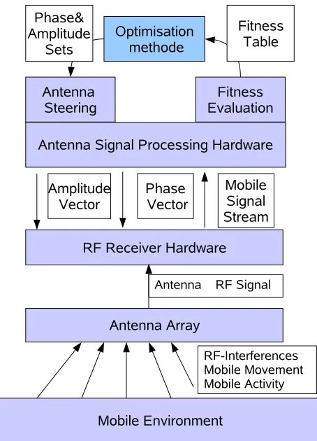
The system overview is presented in figure 1 where one can see the three main parts: the mobile environment, an antenna system and an optimisation unit. The mobile environment comprises mobile (moving) transmitters as well as environmental interferences. The antenna system consisting of an antenna array, receiver hardware and signal processing hardware is responsible to send and receive, but also to electrically and/or electronically adjust the antenna configuration. The optimisation unit on the one hand generates new settings for the antenna system and on the other hand evaluates these settings on the basis of feedback it gets back from the antenna system to influence its following search for better settings.

In this publication the applicability of Particle Swarm Optimization (PSO) and Simulated Annealing (SA) are discussed for this application. Therefore an introduction to the basic principles of adaptive antennas and beam forming methods is given in chapter II followed by the description of the structure of the demonstrator and the associated simulation environment. The chapter closes with a description of the state of the art in the topic of PSO regarding dynamic parallelism and hardware imple-mentation. In chapter III the design of the highly parallel PSO in hardware is discussed. Chapter IV introduces our solution with the help of the parallel SA. The suggested algorithms are examined in the simulation environment on the basis of different scenarios and the results are presented. Chapter VI finishes with the conclusions.

II. FUNDAMENTALS

This chapter provides basic background information on blind adaptive beam forming, our demonstrator for adap-tive antenna systems and describes its software simulation environment.

Figure 1. System Overview

A. Introduction to Beam Forming

The directional radio pattern of an antenna or an an-tenna system in the radiation zone is presented graphically in the form of a radiation pattern and/or an antenna pattern. Such an antenna pattern is shown on the left-hand side of Figure 2. The pattern of a whole antenna array is defined by its geometrical parameters and the individual pattern of its antenna elements. If the antenna is activated only in electromagnetic mode [7], there is no non-mechanical steering possibility to manipulate the pattern.

If superposition of the radio signals from the elements of an array antenna system is considered it is possible to get different patterns and therefore non-mechanical beam forming. This can be achieved through specific changes of the phase and the amplitude of the individual antenna signals as illustrated in Figure 2. By shifting the phase of an individual antenna signal the position of the wave front changes (represented as circles) and thus the directional effect of the entire antenna array is modified. Adaptive beam forming means that the directional antenna characteristic is modified continuously by adaptation of the amplitude and phase-shifting units to a dynamic environment.

Figure 2. Pattern of one antenna element and the basic principle of array antennas [8]

of an antenna in a real world scenario. [9] and others describe the influences of fading, reflection, absorption of radio signals, which have to be taken into account.

Beam forming procedures, which are based on model-based mathematical algorithms, are computation-ally complex and relatively inaccurate because of the leak of knowledge about the environment. Their applicability is therefore limited.

B. Demonstrator System

In order to establish a connection between simulations and real world systems a demonstrator was developed. In parallel a software simulation environment was im-plemented which extensively incorporates the measured characteristics of the demonstrator system with the aim to transfer gained perception in the simulation environment directly to the demonstrator.

The real-time demonstrator system for 2.45GHz ISM band is shown in Figure 3 including a multiplicity of identifiable mobile transmitters realized with 100mW 2.45GHz GMSK transmitters. The antenna array, consist-ing of four individual patch antennas, receives the signals of these mobile transmitters. The signals are filtered and amplified in the corresponding super heterodyne receivers as well as converted to a lower intermediate frequency. Subsequently, the four individual signal paths are merged and, with the help of a digital analogue decoder, passed to digital signal processing as a digital data stream with a data rate between 1.12Gbit/s and 1.47Gbit/s. The signal processing is implemented on a Field Programmable Gate Array (FPGA) [10].

The main component of this system is the Xilinx Virtex-II Pro FPGA, which is a reconfigurable logic device. Decisive for the application as technology for the optimization procedures was the ability of reconfigura-tion and its potentiality to achieve maximum computing speeds by high-parallel processing units.

Crucial for the adaptation in the demonstrator system are on the one hand two controllable attenuators per channel in the high frequency receiver. On the other hand four digital actuators for amplitude correction and four electronically controllable phase shifters in the FPGA are available. Altogether sixteen controllable parameters influence the directional characteristic of the antenna. The first two attenuators use 12bit configuration words each, the amplitude correction needs 18bit and a configuration

Figure 3. Adaptive antenna demonstrator hardware

word for a phase shifter is 8bit long. All in all the antenna system has a number of 2200possible parameter settings. Real-time constraints usually arise from the commu-nication protocol used (e.g. 2ms for 802.11 WLAN or 625µs for Bluetooth). Within these time slots a new best configuration has to be found and the antenna system must be configured with these new settings. If one considers about 1000 fitness evaluations to find a new best setting and on top of it all, that only 10 percent of the available time can be used to find such a setting (rest is used for data transfer) then in our scenario we come to an estimated time period of 18µs to generate a new candidate solu-tion. These strict real-time constraints make a hardware implementation mandatory. Especially because the fitness evaluation can be simply parallelized through pipelining in the FPGA-IP-Core.

C. Simulation Environment

The demonstrator was characterized and forms the basis for a software simulation environment written in C++. Additionally, this simulation environment covers the topics fitness evaluation, environment definition and movement simulation of the mobile transmitters.

Furthermore, a number of transmitters can be initial-ized. These are assigned as desired subscribers or as interferers which should be masked out. Additionally, the simulation can distinguish between active and inactive states of the transmitters. Each transmitter takes an active state with a configurable probability and stays in that state for a stochastically controlled time interval, then it becomes inactive again. The mobile transmitters move along pre-defined paths, which can be specified by the user. Different speeds of the mobiles are possible by defining a maximum and a minimum speed for each path. The available antenna power at the transmitters can be continuously determined to illustrate the beam forming capability. However, the fitness measurement is always afflicted with stochastic (e.g. noise) and biased errors (e.g. offset) in real world scenarios. The fitness calculation of the simulation environment incorporates these possibili-ties only in a limited way: an additional stochastic error is added to the power ratings.

To evaluate the efficiency of the algorithms in different complex environments in an objective manner, a number of static and dynamic scenarios were defined. The envi-ronment of all scenarios has always a size of 4000×4000 units with the adaptive antenna system located in its center.

In the static scenarios the mobile transmitters are set on a random position in each test run. By doing so methodical errors can be avoided. 500 independent tests per scenario were performed, each with 20000 fitness evaluations. The following three scenarios were exam-ined:

• Scenario 1 (static-basic): two transmitters, one dis-turbing and one desired.

• Scenario 2 (static-standard): four transmitters, two disturbing and two desired.

• Scenario 3 (static-complex): nine transmitters, three disturbing and two desired.

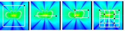
In the dynamic case the mobile transmitters move on predefined paths. The initial positions of the transmitters in each 200 independent test runs were identical. Every 1000 fitness calculations they are moved by 2 or 3 units. In order to be able to collect significant data during each run, 1000 best values must be simulated. The dynamic scenarios are specified as follows:

• Scenario 4 (dynamic–basic 1): two transmitters, one disturbing and one desired. The movement is done stochastically on a square with edge length of 3000 units.

• Scenario 5 (dynamic–basic 2): two transmitters, one disturbing and one desired. They move on a straight line, which passes the basis station very closely.

• Scenario 6 (dynamic–standard): four transmitters, two disturbing and two desired. The mobile trans-mitters move on a small rectangle, whose sides have the distances 200,400,800 and 1600 to the antenna.

• Scenario 7 (dynamic–complex): nine transmitters, four disturbing and five desired. The movement paths consist of five horizontal and five vertical roads,

which cut themselves in 25 crossings.

Figure 4. Dynamic scenarios

Figure 4 illustrates the movement paths of the transmit-ters in the dynamic scenarios. The grey (red) transmittransmit-ters are the disturbers, the black marked ones are the desired mobiles. The bright regions (green) mean a high, the dark (blue) ones a low power density.

Beside the array antenna and its elements, also the channel between the mobile transmitter and the output of the basis station has crucial influence. Related to this channel the input power Pi at the receiver is measured as

follows: [9], [11]:

Pi=Ptx+Gtx+Grx+Prx−Lf s−F (1)

Ptx Transmitting power of the transmitter

Grx Antenna gain of the transmitter

Gtx Antenna gain of the array antenna

Prx Sensitivity of the basis station

Lf s Transducer loss in the free area

F Fade Margin, further losses

For the evaluation of the cumulative fitness first a possibility for the measurement of the receipt quality of an individual mobile transmitter is demanded. This is calculated based on the formula 1 for each elementary antenna element. The addition of these four single power values Pi results in the overall power P of one mobile

station.

For the evaluation of the cumulative fitness for a certain parameter setting the appropriate individual power of all mobile stations must be considered. The disturbing trans-mitters and the desired ones are first evaluated separately from the others. The cumulative fitness arises then as a result of an accordingly weighted addition of these individual values. The computation of the desired mobile participants results from the average of the receiving powers of all active mobile stations of this class.

This average value can be reduced due to punishing contributions, which are assigned in the following three cases:

• The receive power P of the mobile station with the worst reception is too small.

• The receive power P of the mobile station with the best reception is too high.

• The difference between the highest and the lowest power P of all mobile stations of desired mobiles is too high.

The fitness value of the class of disturbing transmitters results from the inverted receiving power of that mobile station with the highest receipt.

additional relevant information than the applied transmis-sion power P, like Bit-Error-Rate, Signal-to-Noise-Ration or other Quality of Service parameters, which are not simulated for performance reasons.

III. BEAMFORMING WITHPARTICLESWARM ALGORITHMS

Particle swarm optimization (PSO) was originally de-veloped by James Kennedy and Russell Eberhart [12] as a robust and efficient method for the optimization of problems in complex, multidimensional search spaces. This stochastic optimization procedure is based on the movement and the intelligence of swarms, which are able to solve the optimization problems by social interactions. Under the utilization of own experiences and those the group aspires, the single individuals of the swarm together can find maximum and/or minimum of the problem. The individuals of the swarm are called particles. Each of these particles possesses a current position−→x and current velocity −→v . The position of the particle represents a possible solution of the problem and it is described by an n dimensional coordinate in the n dimensional search area. The velocity indicates the change in the position from one step to the next. The adjustment of the velocity (equation 2) is the core component of the algorithm. Beyond that the own best position pbest for each particle and the most

successful particle gbest is stored, which is encountered as

the best solution found so far in the entire neighborhood. −

→_{v = w∗v}

id+c1∗rand()∗(pbest,id−xid) (2) +c2∗rand()∗(gbest,id−xid)

The rand() function provides a pseudo random number between 0 and 1, which can be simple realized by a linear shift feedback counter.

A. Related Work

In the literature, the application of the PSO in dynamic and interference-prone environments is well known. First investigations are presented in [13], where the PSO was applied to a number of test problems with a constantly changing environment. To ensure the efficiency and ro-bustness of the particle swarm optimization as also tracing the found optima in dynamic systems, different modifica-tions of the original PSO are discussed in the literature.

Recalculation of the fitness, Observation of the value gbest, Restore the value pbest and Random

Reinitial-ization [14]: The monitoring of the environment takes place on the basis of the double computation of the fitness value of the same particle, before as well as after the execution of an iteration. If the difference of these values crosses a certain limit, then certain reaction measures are made. If the PSO is not able to follow dynamic changes, then the value gbest of the swarm cannot change.

If the best value of the swarm has not resulted in an improvement after a certain number of iterations an alarm is raised. The value pbest of the particles is replaced by

their present/intermediate position. Alternatively for this

the fitness of the best position for each particle can be computed again. pbest is replaced only, if this value is

worse than the current position. If the swarm has already converge in a small range already, then it is not possible to break out by putting pbest of the values back from this

area. It is meaningful to make a reinitialization of part of the particles regarding position, velocity and best values. Additionally there are several further interesting ex-tensions of PSOs as Loaded Particles Swarm and Multi Charged Particle Swarm [15], Multi-Cluster Particle Swarm [16] or Multi-Hierarchical Particle Swarms [17], which may increase the simulation performance but they are not well suited for parallelization in distributed logic devices, but the principle idea of parallel swarms will be re-used in chapter III-C.

Within the domain of electrodynamics only few in-vestigations exist applying PSOs since recent time. First publications for the production of antenna directional characteristics with array antennas on basis of PSO are introduced in [18]. A goal of these investigations was to optimize the phase shifts and amplitude controls of an antenna array of 20 elements.

B. Real Time Optimization Problem

The task of the optimization is to generate an optimal directional pattern within given conditions. The optimiza-tion problem can be represented formally as follows:

max F(E(t),S(t),t)|B (3)

Equation 3 indicates that the maximization of the fitness F must take place at time t, depending on the environment E(t) and the selected scenario S(t) at this time under different conditions B. The definition of the conditions under which the optimization of the fitness values and the fitness evaluation itself has to be executed was made arbitrary but close to the real world communi-cation systems as wireless LAN. This set of conditions, which the particle swarm algorithm must meet, describes a dynamic environment with the following constraints:

• Minimum adaptation rate of the communication system: So that a radio communication does not break away or can be established it is necessary that the PSO adapted the radio system within a given time interval on a minimum value of the fitness. For the simulation an interval of 1ms is defined, in order to reach a good fitness value.

• Discontinuity of the transmitter: It can happen that desired and disturbing transmitters are deactivated and/or activated. This means for the PSO that the participants abruptly disappear and possibly appear on another position again. The system must react to these changes sufficiently within the fixed time interval of 1ms.

Figure 5. Hardware architecture

The consequence of the described conditions is an en-couragement for real-time optimization of the directional characteristic with a fixed limit of 1ms respectively 1µs per fitness evaluation. The PSO should be designed as highly-parallel hardware, because a pure software solution due to the sequential processing would need two to three orders of magnitude more time for the adaptation [5]. The adaptation must be carried out after max. 1000 fitness evaluations.

C. Concept of the Highly-Parallel PSO

Certain factors - like the neighborhood structure and the synchronization- have influence on the hardware imple-mentation. Due to the small particle number it is possible to assign to each particle its own computation component so that the particles could determine their new positions parallel to each other.

If a simple two-dimensional arrangement of the particle components in the FPGA is applied, it results a regular matrix structure. As natural neighborhood of a particle offers here all spatially at particles bordering individuals, so that only short communication connections between spatially directly neighboring particles are needed. Figure 5 illustrates this basic hardware structure. Communication components K between the particles P serve for the change of the global best position of the particles of a neighborhood as well as for the synchronization with the fitness evaluation components.

To fulfill the hard real-time conditions, the degree of parallelism of the hardware implementation must be as high as possible. This means that as much as possible components must be placed for the computation of the speed on the FPGA, on the other side only a limited number of operators on the FPGA can be situated. For the size of a multiplication operation of two numbers in hardware their word length is crucial.

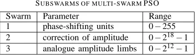
Therefore, it was examined that the introduction of or-thogonal multi-swarms is the most promising modification of the PSO. With the realization of this multi-swarm structure each single swarm optimizes only a single type of parameters as it is enumerated in table I.

During the initialization for each particle, random po-sitions are generated only in the dimensions of the ap-propriate type of parameter of these subswarms. Starting the optimization process the fitness of the particles of the individual subswarms is successively evaluated. For the first iteration of fitness evaluation of the first subswarm

TABLE I.

SUBSWARMS OF MULTI-SWARMPSO

Swarm Parameter Range 1 phase-shifting units 0−255 2 correction of amplitude 0−218−1 3 analogue amplitude limbs 0−212−1

the parameter types of the two remaining subswarms are set in each case into the center of the range of values. For the evaluation of the next subswarms the dimensions of the remaining parameter types are placed to the best found values of the previous subswarms. So that between the fitness evaluations no waiting periods arise, the last particle of the first swarm is ignored. With a subswarm A with 20 particles in the fitness evaluation of the following subswarms B the parameter types of the swarm A are set on the best found parameter setting of only the first 19 particle. This suggested strategy possesses the following advantages:

• Predominance of the phase-shifting units: They possess tendentiously a higher influence on the an-tenna pattern than the amplitude members. Thus, the adaptation ability of the PSO increases.

• Increase of the test speed: The setting of the phase-shifting units and the amplitude corrections in the FPGA can take place around a factor of 100 faster time interval than the setting of the amplitude mem-bers in the receiver boards of the antennas. As it was described in Section II-B, 1µs is needed for setting the amplitude members. The setting of the digital amplitude corrections can take place in 12ns. Setting the phase-shifting units even in approx. 10−15ns, because these variables are processed digital in the FPGA.

So a fitness evaluation in the sense of the classical particle swarm algorithm, with which all parameters are set, needs well one microsecond. In consequence of the allocation of the swarm in accordance with the existing parameter types each fitness evaluation sets only the parameters of the appropriate type of swarm. For example a subswarm, which optimizes the phase-shifting units, requires only 10−20ns for the computation of the fitness. Consequently in the time, in which a new directional characteristic is to be provided a higher number of fitness evaluation can take place than compared with the normal PSO.

swarm algorithm - on the basis of a swarm size of 40 particles - thus memory requirements of 40∗3∗

200bit=24000bit are necessary. In the case of the multi-swarm with three subswarms (20, 10 and 10 particles), memory requirements of 20∗3∗32bit+ 10∗3∗72bit+10∗3∗96bit=6960bit.

IV. BEAMFORMING WITHSIMULATEDANNEALING ALGORITHM

Simulated Annealing is generally considered as the oldest metaheuristic and is one of the first algorithms, that explicitly tries to avoid local minima. Contrary to PSO algorithms, it is a technology known for a relatively long time and thus a very well-investigated technology.

The basic ideas were published already in 1953 by Metropolis and colleagues [19]. Paradigm for SA is a phenomenon well-known from physics. If materials are heated up beyond their melting point crystals of differ-ent sizes can develop. Structural characteristics of the annealed material depend on the speed of the cooling process. With decreasing temperature T the total energy E of the material drops. The goal is to reach the global energy minimum without being traped in a local energy minimum. This is only possible with a sufficient slow cooling procedure. The difficulty is to supply exactly the right amount of heating energy to the annealing material thus it does not warm up again but also does not cool down too fast – which means it always has enough energy to leave local minima towards the global minimum.

The algorithm of Metropolis simulates exactly these changes of energy conditions of an annealing material. According to this, the probability for an energy increase byδE at a temperature T is given by the formula 4,

p(δE) =e−δkTE, (_k=₁,₃₈₀₆₆·₁₀−23_J/_K) ₍₄₎ whereas k is the Boltzmann constant.

Solutions in the neighborhood of the current state are generated during the simulation of Metropolis and the energy change resulting from it is computed. If the energy decreases, the system takes the new condition. If the energy level increases, then the new condition is accepted only with a probability p as defined in equation 4. The possibility to accept states with higher energy levels allows the system to leave local minima again. This procedure is repeated a previously defined number of times for each temperature.

In 1983 Kirkpatrick and colleagues [20] suggested to apply this kind of simulation to search for valid solutions of optimization problems. With the help of Simulated Annealing global optimal solutions should be found.

Algorithm 1 illustrates a typical operational sequence for SA. However, unlike the natural model it is not about minimizing an energy level. Our problem is about maximizing a possible fitness value. Thus p(∆Fitness) = e−δFitnesskT _{describes the probability to accept a fitness level} that is worse of about∆Fitness=f it(Sbest)−f it(Snew)≥

0.

Algorithm 1 Algorithm for Simulated Annealing in pseudo code

Initialization with a coincidental solution; Sbest=Scurrent=Scoincidental; T=Tstart;

repeat repeat

Search for new solution Snewin the neighbourhood

from Scurrent;

compute fitness f it(Snew);

if f it(Snew)>f it(Sbest)then Sbest=Snew; Scurrent=Snew;

else

if p(∆Fitness)>r then

Accept Snew despite worse fitness values; Scurrent=Snew

end if end if

until Stop criterion for neighbourhood search fulfills; lower temperature T over δT ;

until T==Tmin

The correct parameter choice how many states of higher energy are accepted and/or how strongly such an increase in energy may be and at which distance of the current state new solutions are examined strongly depends on the cost function of the problem to be solved and on the used search strategy. Finding suitable parameter settings for example for the temperature and its dropping speed, the number of iterations and the choice of suitable abort criteria, is substantial for the successful use of SA to the optimization of a problem.

SA algorithms cover a wide application area ( [20]– [23]). Since SA is a profoundly sequential algorithm, the next section gives a more detailed survey of attempts made in the past to parallelize this method.

A. Related Work

The basic principle of Simulated Annealing shows that SA is a quite a simple algorithm, which was al-ready successfully used to solve a whole set of NP-hard problems. Regarding to [24] the main focus of research concentrates on speed improvements and thus gaining more efficiency. One of the common methods to achieve this is the application of parallel processing. Since SA in its original form is however a strictly sequential algorithm, where iteration i+1 depends directly on the results of iteration i, the parallelism of SA is an extremely difficult task. Past attempts in literature can be divided into two categories:

• parallel SA algorithms: The process of the SA is split into individual tasks, which are divided on dif-ferent processors. Examples of it are Parallel Markov chain [25], [26], Parallel Markov Trials (PMT) [25], [26], Adaptive parallel Simulated Annealing (APSA) [26], Speculative Trees (ST) [27].

In summary Sanvicente-Sánchez and Frausto-Solísin in [24] come to the conclusion that under normal conditions all these parallel attempts to SA achieve relatively bad performance. It turns out that a large drawback for most approaches (DCP, PMT, APSA, ST) results in a huge communication complexity, which often destroys all ben-efits of parallelism. PIA does not have any run time advan-tage in relation to a sequential SA and PMC works well only at high temperatures and on few processors. Also the systolic algorithm works only with few processors and additionally reduces the accuracy of the SA.

Sanvicente-Sánchez and Frausto-Solísin suggest also another solution in MPSA [24]. They parallelize the outside loop, meaning the sinking of the temperature, by defining fixed temperature steps before an optimization run and distributing these on different processors. All processors generate solutions at the same time according to the Monte Carlo principle, meaning the inner loop of the SA algorithm.

Instances with a high temperature level search in a large neighborhood for new solutions, while instances with a very low temperature concentrate their search on solutions in direct neighborhood. If a temperature level produces a new best solution the result is passed on all instances with a lower temperature, which examine whether this solution is better than their own best solution. If that is the case, this new solution provides the basis for their further search.

By partitioning the outside loop (off-line) before start-ing the actual optimization run, MPSA gets along with substantially less communication overhead during the ac-tual optimization run than most other attempts. The exact partitioning and distribution of the individual temperature levels is a parameter setting of the SA.

Reducing the run time of optimization runs with SA for different problems leeds to a hardware implementation of the algorithm. The typical design of such hardware mandatorily gets back on questions about parallelizing the heuristic, due to the fact that the main speed advantages of hardware algorithms originate from consequently utilizing such parallelizing potentiality. The following hardware variants consequently provide basic support for parts of the algorithm.

Some concepts for the hardware implementation of SA can already be found in literature. They reach from very problem-specific drafts, as for example for Fast FPGA Placement [22] up to hardware support for SA and Tabu search (TS) in form of a CPU kernel extension [28], where one of the design goals for Schneider and Weiss was to maximize flexibility. To achieve this flexibility only several modules where designed in hardware. Combining these modules allows to adept to different problems and

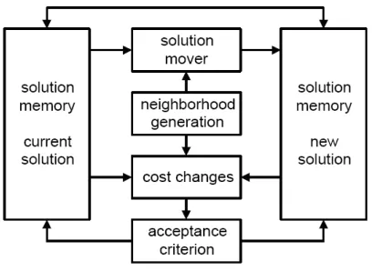
Figure 6. Module overview

problem solving strategies. Here is a rough overview of the given individual modules, since they reflect the individual parts of a typical SA very well. For more exact data to the modules see [28].

• Solution Memory: Memory for the representation of the solution area realized as concatenated list and matrix

• Neighborhood Generation: The generation of a suitable neighborhood depends on the used algorithm

• Solution Mover. Module for the correct control of both memories (see figure 6) and to supply the respectively best solution.

• Acceptance Criterion: Hardware component to de-cide whether a solution is accepted or rejected.

• Acceptance Prediction: Module to support parallel SA strategies, which need a forecast of the probabil-ity of acceptance of a solution.

• Status Information: Statistic information about the relative change of solution quality.

B. Problem Representation

Simulated Annealing is a variant of local neighborhood search. It is therefore an essential component of the con-ception of a successful SA algorithm to define a suitable neighborhood on the selected problem representation. In principle, a representation could be a vector of 200 bit values or a parameter vector with 16 entries and different value ranges for each case. A SA algorithm consists of two interleaved loops. The outside loop limits the neighborhood, where new solutions are searched, with progressing optimization. In the internal loop new best solutions are searched within such a neighborhood.

Thus, the question arises, how a neighborhood to a parameter setting in form of a vector looks like. From a fitness value it is definitely not possible to conclude individual parameter values nor to win information about how good or bad the fitness value of an individual pa-rameter is. In each case only complete papa-rameter settings of 16 parameters can be evaluated as a whole. Therefore it is also not possible to define a neighborhood based on good or bad parameter values since it cannot be foreseen, how changes in detail or in combination affect the fitness. Considering this, it is a consequent step to define neighbors to the current vector as slightly modified versions. Slightly modified means, its parameter values are mutated within certain borders. Such distances can be defined differently. The Euclidean distance between two vectors x and y in equation 5 is a well-known distance definition.

d(x,y) =|x−y|= s

n

∑

i=1

(xi−yi)2 (5)

Regarding the optimization, a distance version can be defined that is limited in the number of values which can be changed at a time. Thus it is possible to change several or relatively few parameters and evaluate these changes. In the case of a change in form of an Euclidean distance it is possible that the modification would cause a better setting on a parameter, however by the simultaneous change of other values this improvement might get elim-inated again. This assumption was confirmed clearly by experiments. Therefore the definition of a neighborhood was examined on one hand by restricting the number of simultaneously modified parameters on the other, by simultaneously restricting the range of values around the actual parameter, in which such a change can occur. Thereby in each case a number k is changed by the 16 entries of the problem vector which are selected randomly. The maximum distanceδx of a value change is affected by the temperature sequence of the SA process and decreases with progression of the optimization. Equation 6 defines the neighborhood regulation of a parameter i∈[1,16].

xi_current=xi_current+r,r∈[−∆xi,+∆xi] (6) Simulations showed that this variant of neighborhood definition yields clearly better results in relation to a neighborhood search with Euclidean distance. That is the reason why it is used for the further procedure.

C. Dynamics

In dynamic environments the problem exists that the optimal solution changes over the time. For tracing of such an dynamic optimum it is emergency to give up the before obtained convergence, at least up to a certain degree and to investigate with the search for the new optimum in a larger area of the search area. The size of the area which can be searched depends considerably from the process respectively from the current conditions of the temperature. With falling temperature, SA concentrates the search even more on the region around the up to then best result. In order to expand the search area after the change of the environment, it is necessary to raise the temperature. Besides that, a new computation of the fitness of Sbest is necessary. We interpret the adjustment

to a dynamic surrounding field thus as temperature rise in the SA.

If a typical SA algorithm is regarded, then, as can be easily recognised in the algorithm 1, no intermediate results can be stored. Only exception forms the presently best well-known solution. The increasing of temperature during simultaneous re-valuation of Sbest comes therefore

near to a complete restart of the search. Only the starting point, at which the new search begins, is given by Sbest.

Examining a standard algorithm for SA in a very simple static system it is noticeable that it could already profit from storage of intermediate results. One regards in addition the sketches in Figure 7.

Figure 7. Neighbourhood with a very simple example

The example was selected because the neighbourhood can be represented on the left, and the current value Scurrent on the right very descriptive. If the system takes

now a new value in the neighbourhood examined before (Scurrent =Snew) (to be seen in b)), then in the next

step, it follows again a neighbourhood regulation with appropriate fitness evaluation around Scurrent. Part of this

neighbourhood the algorithm already examined the previ-ous iteration. In a static environment these values do not changed.

tem-perature gradient plays an important role. Therefore it still concerns a procedure of the type Simulated Annealing.

D. Hardware Concept

Due to the simplicity of the algorithm, Simulated Annealing can be implemented in hardware in its standard design with slight modifications. The goal of this work is only to suggest a possible hardware concept for SA. The hardware implementation of the algorithms is to clearly speed up the search for new solutions in relation to a pure software implementation. It is not enough to convert the algorithm one to one in hardware. As previously mentioned the advantage of a FPGA is among other things in its immense parallelism. The question about a meaningful and fast hardware implementation for SA returns thus obligatorily to the parallel of SA.

1) Parallelisation of the Solution: As the literature presented in chapters IV-A clearly shows, the parallelism of SA is a very difficult topic. The main problem lies in the fact justified that each further search for a new solution depends fundamentally on the preceding solution. We suggest first a similar procedure, as with ACO [30].

Figure 8. Ring buffer

The solution is divided again into individual parts, which can be parallel worked on. With a vector with 16 components an offers allocation in 16 individually parts. On these parts can be searched parallel for neighbours of the present value. Because it is not possible to evaluate individual partial solutions, it additionally requires the single solutions of the other parts. Therefore each part makes its up-to-date best value available. To evaluate a new neighbour a partial solution must complete with (best) the values of the other parts and delivers it to the interface of the fitness evaluation. Meanwhile the other parts proceed similar.

Figure 9. Realization pattern of the ring structure

2) Ring Buffer: Our idea for the organization of such a subunit exists in the construction of a ring buffer, as it is outlined in figure 8.

If only one direction of rotation is regarded, then the arrangement resembles a pipeline which admits the functional modules (grey) operate at the same time. First new solutions are generated from the neighbourhood and registered into the buffer. The next active functional unit (reading from solutions and regulating their fitness) reads these solutions from the memory and transfers it to the antenna to the actual fitness evaluation. After a delay caused by this evaluation, the determined fitness value can be written at corresponding in the meantime forward rotated place. The next logical step consists with SA of deciding whether the solution is better than the best well-known solution. If it is true, then it replaces the best past solution on the one hand and serves on the other hand the new starting point for future neighbourhood regulations. If this should not be the case, then the selection unit decides whether the worse solution in the sense of SA serves as basis for new neighbourhood searches.

The direction of rotation of the memory is determined thereby, in which direction a solution is selected as new starting point for a renewed neighbourhood regulation. If this step takes place towards a new, yet did not visit region, then this part of the new neighbourhood is first examined. If there is still sufficient time remaining, then the points on that already admitted neighbourhood side are evaluated again. Before a change of the direction of rotation, the ring buffer needs some clocks in order to store the remaining fitness value with the appropriate solutions.

A pipeline-like representation, how it is transferable to the hardware from the principle, shows the figure 9. It is important to be able to change the direction of rotation of the memory, as represented in figure 8, to controle the memory access accordingly.

Figure 10. Individual memory area the ring structure

the memory at the write address can take place only after final read access and receipt of a further clock pulse. If thereafter the direction of rotation remains the same, then the cycle begins again. However if the direction of rotation changes (Direction=0), then the storage addresses in the following step is not increased but decremented. Also here an appropriate overflow mechanism must be present for the memory counters. However the addresses to be now lowered, a resetting takes place on the greatest possible storage address in the difference.

The interconnection of the different ring buffer to a system happens, similarly the solution for ACO [30]. Each ring buffer produces parallel a part of the solution. If a part is to be evaluated, then the own partial solution must be extended by the values of the other ring buffer. Only then a solution can be handed over to the fitness evaluation. In addition to that, each part can access the best parts of the other ring buffer. After which strategy the individual rings evaluate solutions depends on settings thing. A simple and plausible strategy would be to to take this in turn. The evaluation result flows thereupon again directly into the ring buffer. There it supplements as had, the solution around its fitness value.

V. TESTING ANDEVALUATION OF THESIMULATION RESULTS

In order to find a suitable parameter setting the evalua-tion of the PSO and of the SA were applied in a first and second step. The third evaluation step was processed for the measurement of the PSOs and of the SA efficiency and the impact of different static and dynamic environments. As comparison and reference a genetic algorithm from [5] was applied.

A. Parameter Settings of the PSO

In order to specify the parameters of the PSOs with an optimum convergence, these must be simulated in their ranges of values. The selection of parameters is based on two criteria:

1) Parameter with direct influence on the realizability of implementation in hardware

2) Results of selected sample simulations or from the literature study

In Table II the parameters, their appropriate values, the standard setting and the test result are indicated.

In the context of the investigations of the classical PSO there is a number of 6x8x8x7x6x8=129024 possible

parameter combinations. To reduce the large number of possible parameter setting in each step only one parameter is varied independently of the other parameters. The re-maining parameters are set on the default value indicated in the TableII . All test rows were examined both in a static and in a dynamic scenario. During the test process in all scenarios four mobile transmitters, two desired and two disturbing transmitters were used.

TABLE II.

EVALUATION OF PARAMETER SETTINGS

parameter evaluation values standard simulation

number of particle 20,30,36,40,50,60 40 30

neighborhood global, matrix, wheel ring with 6 matrix structure ring with 4,6,8,10 12 neighb

neighb.

control structures

Inertia Weight: 7.5−0.375,7.5−0.5, 7.5−0.375 0.375 movement weights 0.5,0.375

csoz.: cind. 2 : 2,3 : 1 2 : 2 2 : 2

maximum offset

in all dimension 0,8,16,32,64 32 −

only in one dimension 255 − 255

multi-swarms

structure ring, matrix matrix

particle ampl./ phases 10,12 / 20,30,40 − 10 / 20

For the multi-swarm algorithm a ring structure with 20 particles in the phase swarm and 10 particles in the two amplitude swarms were selected in each case. The size of the neighborhood in the phase swarm is six, in the two amplitude swarms is in each case four neighbors. The remaining parameters are chosen from the results of the classical PSO.

B. Parameter Settings of the SA

Through especially in the dynamic case strongly limited number of possible fitness evaluation to obtain the best solution our system trades off in other implementations often practiced heating up procedure which stays in analogy to the physical model. The SA always begins at a fixed temperature t0. From the beginning the maximum number of the fitness evaluations is know, which can be used to determine a new solution. In order to arrive at such a solution, a more strictly plan can be defined from the beginning, than otherwise often the case is. Therefore, the strategy mentioned in chapters IV-D was implemented. It is based on discretely linear temperature gradient and equal distributed number at neighbourhood searches per temperature. The temperature pattern based on the so-called Cauchy Annealing. The only parameter, which can be indicated for a SA algorithm, is the mutation ratemr. It corresponds to the variable k from the chapter IV-B, which indicates the number of parameters which can be modified at the same time in the simulation.

C. Conclusion from the Simulations

TABLE III.

COMPARISON OF THE SIMULATION RESULTS

Scenario 1 Scenario 2 Scenario 3 Scenario 4 Scenario 5 Scenario 6 Scenario 7

GA 102,1 56,0 30,5 45,6 56,8 29,6 25,4

SA 94,4 56,2 29,8 58,0 54,5 25,9 24,7

PSO 138,1 101,2 48,6 93,2 103,4 42,9 46,9

Multi PSO 136,9 106,8 58,3 76,1 88,8 44,1 48,4

500 independent tests are executed. From the results of these simulations the following realizations can be drawn: 1) In each of the seven scenarios the particle swarm procedures showed the best efficiency. The algo-rithm of the SA obtains a worse performance, which lies on the same level as the genetic algorithm. 2) In simple scenarios with only two transmitters the

classical PSO exhibits better results. The Multi PSO continuously obtains however in all scenarios with middle and high complexity a better performance. This lies on the phase-shifting units, so that the directivity pattern is adapted more purposefully towards the desired transmitter and disturbers are better blinded out at the same time.

3) The GA presented in [5] serving as guidelines is also improvement. We used new selection and mutation operators, the probability of the muta-tion is increased and the probability of crossover decreased. The parameter setting was the follow-ing population size: 128, rank selection, onepoint crossover, random mutation, crossover rate: 0.7 and mutation rate: 0.4

The primari goal of this work was to examine the general suitability of the three procedures (SA,PSO and Multi-PSO) for the solution of the task posed. In addition software implementations of the procedures were pro-vided, in order to draw comparisons between the proce-dures, on the basis simulations. It turned out that all three procedures for the optimization of parameters are suitable. Both swarm algorithms and SA follow the changes of the environment. This becomes clear by the constantly high fitness values of the curve. The simulation results prove that a particle swarm optimization represents a suitable attempt for the optimization of antenna characteristics, even if this is afflicted with the necessary restrictions for a hardware implementation.

VI. CONCLUSION ANDFUTUREWORK In the context of this publication the suitability of the particle swarm optimization, simulated annealing and genetic algorithm for the employment to blind adaptive beam forming was examined.

For the solution of the problem the algorithms were converted including hardware-technical aspects of the blind adaptive beam forming. Additionally to the stan-dard particle swarm optimization an other particle swarm variant algorithm was designed, which consists of several individual swarms (Multi PSO). This offers the following advantages in relation to the classical PSO procedure:

• Higher performance in complex environments due to the possibility of the stronger emphasis of the phase adjustment.

• Higher number of possible fitness evaluations due to the acceleration of the fitness function.

• Reduction of the resources needed at memory and logic blocks in the FPGA.

• Maximum adaptation rate by highly-parallel hard-ware synthesis structure.

For parametrizing the optimization algorithms as well as for the investigation of the efficiency particularly in dynamic environments systematic simulation tests were accomplished, evaluated and interpreted. The next step is to extend and integrate into the existing demonstrator system the hardware implementation of the algorithms. Thus, the results yielded by the simulation can be studied by measurements and be examined for their practical feasibility in a real world field test.

REFERENCES

[1] C.-N. Chuah, D. N. C. Tse, J. M. Kahn, and R. A. Valenzuela, “Capacity scaling in mimo wireless systems under correlated fading,” IEEE Transactions on Informa-tion Theory, vol. 48, no. 3, pp. 637–650, 2002.

[2] J. Litva and T. K.-Y. Lo, Digital Beam forming in Wireless Applicatons. Artech House Norwood, 1996.

[3] A. E. Zooghby, C. Christodoulou, and M. Georgiopoulos, “Neural network-based adaptive beam forming for one and two dimensional antenna arrays,” IEEE Transactions on Antennas and Propagation, Dec 1998.

[4] K. K. Shetty, “A novel algorithm for uplink interference suppressing using smart antennas in mobile communica-tions,” Ph.D. dissertation, etd-04092004-143712, 2004. [5] G. Kókai, H. H. Frühauf, and F. Xu, “Adaptive smart

an-tenna receiver controlled by a hardware-based genetic op-timizer,” International Journal of Embedded Systems Spe-cial Issue on Hardware-Software Codesign for Systems-on-Chip, vol. 1, no. 1/2, pp. 50–65, 2005.

[6] G. Kókai, T. Christ, and H. H. Frühauf, “Using hardware-based particle swarm method for dynamic optimization of adaptive array antennas,” in Proc. First NASA/ESA Conference on Adaptive Hardware and Systems, K. Didier, Ed., 2006, pp. 51–58.

[7] R. W. Heath and D. J. Love, “Dual-mode antenna selection for spatial multiplexing systems with linear receivers,” Dept. of Electrical and Computer Engineering The Uni-versity of Texas at Austin Austin, Tech. Rep., 2004. [8] D. Hyman, Rugged RF-MEMS Packaging Strategies.

XCom Wireless Inc. Signal Hill, 2002.

[9] F. Vilbig, Lehrbuch der Hochfrequenztechnik. Akademis-che Verlagsgeselschaft Geest und Portig K.-G., Leipzig, 5. Auflage, 1953.

[11] S. Inc, “White paper on rf propagation basics,” April 2004. [12] J. Kennendy and R. C. Eberhart, “Particle swarm optimiza-tion,” in Proceedings of IEEE International Conference on Neural Networks. Piscataway, NJ, 1995, pp. 1942–1948. [13] K. E. Parsopoulos and M. N. Vrahatis, “Particle swarm op-timizer in noisy and continously changing environments,” in Proceeding of the IASTED International Conference on Artificial Intelligence and Soft Computing (ASC 2001)Can-cun, Mexico. Cancun, Mexico, 2001, pp. 289–294. [14] X. Hu and R. C. Eberhart, “Adaptive particle swarm

optimization: Detection and response to dynamic systems,” in Proceedings of IEEE Congress on Evolutionary Com-putation (CEC 2002). Honolulu, Hawaii, USA, 2002, pp. 1666–1670.

[15] T. M. Blackwell and J. Branke., “Multi-swarm optimiza-tion in dynamic environments,” in Proceedings of Appli-cations of Evolutionary Computing: EvoWorkshops 2004: EvoBIO, EvoCOMNET, EvoHOT, EvoISAP, EvoMUSART and EvoSTOC. Coimbra, Portugal, 2004, pp. 489–500. [16] D. Parrott and X. Li, “A particle swarm model for

tracking multiple peaks in a dynamic environment using speciation,” in In Proceeding of the 2004 Congress on Evolutionary Computation (CEC 2004). IEEE Service Center, Piscataway, 2004, pp. 98–103.

[17] S. Janson and M. Middendorf, “A hierarchical particle swarm optimizer for dynamic optimization problems,” in Proceedings of Applications of Evolutionary Computing: EvoWorkshops 2004. Coimbra, Portugal, 2004, pp. 513– 524.

[18] D. Gies and Y. Rahmat-Samii, “Particle swarm optimiza-tion for reconfigurable phase-differentiated array design.” Microwave and Optical Technology Letters, vol. 38, no. 3, pp. 168–175, 2003.

[19] N. Metropolis, A. W. Rosenbluth, M. N. Rosenbluth, A. H. Teller, and E. Teller, “Equation of state calculation by fast computing machines,” Journal of Chemical Physics, vol. 21, pp. 1087–1092, 1953.

[20] S. Kirkpatrick, C. D. Gelatt, and M. P. Vecchi, “Optimization by simulated annealing,” Science, Number 4598, 13 May 1983, vol. 220, 4598, pp. 671–680, 1983. [Online]. Available: citeseer.ist.psu.edu/kirkpatrick83optimization.html [21] G. Kliewer and P. Unruth, “Parallele Simulated Annealing

Bibliothek: Entwicklung und Einsatz in der Flugplanop-timierung,” Master’s thesis, Universität-Gesamthochschule Paderborn, 1998.

[22] M. G. Wrighton and A. M. DeHon, “Hardware-assisted Simulated Annealing with application for fast FPGA place-ment,” in Proceedings of the 2003 ACM/SIGDA eleventh international symposium on Field programmable gate ar-rays. ACM Press, 2003, pp. 33–42.

[23] X. Wang and M. Damodaran, “Aerodynamic Shape Opti-mization Using Computational Fluid Dynamics and Par-allel Simulated Annealing Algorithms,” AIAA Journal, vol. 39, pp. 1500–1508, 2001.

[24] H. Sanvicente-Sánchez and J. Frausto-Solís, “MPSA: A Methodology to parallelize Simulated Annealing and its application to the Traveling Salesman Problem,” in Pro-ceedings of the Second Mexican International Conference on Artificial Intelligence. Springer-Verlag, 2002, pp. 89– 97.

[25] R. Azencott, Ed., Simulated Annealing: Parallelization Techniques. John Wiley, 1992.

[26] R. Diekmann, R. Lüling, and J. Simon, “Problem Independent Distributed Simulated Annealing and its Applications,” Paderborn Center for Parallel Computing, Tech. Rep. TR-003-93, 93. [Online]. Available: citeseer.ist.psu.edu/diekmann93problem.html

[27] D. R. Greening, “A taxonomy of parallel Simulated An-nealing techniques,” University of California, Los Angeles:

Computer Science Department, Tech. Rep. CSD-890050, August 1989.

[28] R. Schneider and R. Weiss, “Hardware Support for Simu-lated Annealing and Tabu Search,” in Proceedings of the 15 IPDPS 2000 Workshops on Parallel and Distributed Processing. Springer-Verlag, 2000, pp. 660–670. [29] F. Glover and M. Laguna, Tabu Search. Dordrecht,

Niederlande: Kluwer Academic Publishers, 1998. [30] M. Böhner, G. Kókai, and H. H. Frühauf, “Dynamic

hardware-based optimization for adaptive array antennas,” in Integrated Intelligent Systems for Engineering Design, X. F. Zha and H. Howlett, Eds. Amsterdam, The Netherlands: IOS Press, 2006, pp. 362–388.

Dr. Gabriella Kókai studied computer science in the University of Szeged, Hungary. She received Ph.D degree from the Friedrich-Alexander University Erlangen-Nürnberg (1998) and from the University Szeged Hungary (2000). She is currently a gast lecturer on the Friedrich-Alexander University Erlangen-Nürnberg and works by the company Elektrobit Automotive. Her areas of investigation are machine learning, data mining, and soft computing, with a focus on real world application.

Martin Böhner studied computer science at Friedrich Alexander University Erlangen-Nuernberg until 2004. Since then he is em-ployed at Elektrobit Automotive. At present he engages in the application of cryptographic methods to embedded devices with main focus on automotive environments.

Tonia Christ studied computer science at the Friedrich Alexander University Erlangen-Nuernberg until 2004. At present she works on the Fraunhofer Institut for integrated circuits IIS in Erlangen. The ranges of their interest are FPGA Design and hardware optimization for HF applications.