1388
On The Use Of Machine Learning For Temporal
Performance Prediction In Lte Advanced
Networks
Maureen N. Mureithi, Peter K. Kihato, Agnes Mindila
Abstract: Performance prediction is an indispensable topic to any mobile network operator. It allows the operators to be aware of future network scenarios and take actions before they occur. This paper explores various machine learning approaches to predict performance. Real world data is mined and analyzed to identify the geospatial distribution of samples and their temporal relationships. Time series techniques based on general additive model, auto-regressive model and deep learning are evaluated. Long-term short-term deep learning model was used, and it performed better compared to the others giving results that are adequate for most planning and optimization tasks.
Index Terms: deep learning, Machine Learning, Neural networks, Reference Signal Received Power (RSRP), Reference Signal Received Quality (RSRQ), signal-to-interference-plus-noise ratio (SINR), time series.
—————————— ——————————
1.
INTRODUCTION
There is a tremendous increase in inventions and innovations in radio access technology leading to overall operational efficiency. However, much more work needs to be done in radio access planning and optimization to leverage on emerging technologies like deep learning. Automation of manual and routine tasks has the potential to reduce significantly the operational costs of Mobile Network Operators (MNOs) and improve the quality of user experience. Currently, network management tasks require human interactions such as conducting and analyzing drive tests, key performance indicator (KPIs) analysis and resolution of customer complaints. Customer complaints already indicate that the users on the ground are experiencing degradation of services and are likely to churn. Customer satisfaction is key in customer retention and studies show that it costs 5-10 times more to acquire a new customer than to maintain an old one [1]. KPIs are an indication of the network performance and can be used to troubleshoot and optimize the network. They are limited because of the availability of data and the granularity of the available data [2]. KPIs are averaged to the granularity of cell level and are not real time, they offer a reactive approach towards resolving faults in a network. Another technique used to collect performance measurements is through drive tests. They are conducted and analyzed manually. This has proved to be costly, tedious and ineffective. Hence, the Third Generation Partnership Project (3GPP) has put in place various measures to minimize drive tests such as standardization of measurements for both UMTS and LTE networks (Release 10), possibility to collect user uplink and downlink throughput measurements and the availability of location information (release 11). With minimization of Drive Test
(MDT), MNOs are enabled to remotely collect measurements indicating network quality of service as experienced by the users and the correlated location information [3]. The data that is collected through the MDT technic is huge and requires big data technics to analyze.
2
RELATED
WORK
Machine learning offers a plethora of opportunities in cellular network operations. A lot of research is being done with regards to the impact of machine learning on cellular radio networks [4], [5], [6]. This is because the adoption of machine learning techniques in radio networks is expected to reduce operational expenditure (OPEX) and improve user experience [6]. Performance prediction in wireless networks has always been an important but challenging task for radio engineers. Conventionally, prediction has been based on signal propagation models which attempt to estimate the path losses due to geospatial and none geospatial conditions [7], [8], [9]. These methods are based on assumptions and a one-fit-all solution, that is, an urban model applies to all urban centers despite their differences. A key concept has emerged in the past decade called the radio environmental maps (REMs) [10]. This has led to increased research on radio signal analysis with machine learning. In [11] and [12], the authors suggest the use of REMs for coverage analysis through spatial interpolation techniques to group together areas with poor coverage and to predict the signals of locations close to but not covered by a drive test. The use of machine learning is postulated in [11] to predict performance and [13] to predict uplink power given the pre-existing conditions. In this paper a novel approach that employs LSTM deep learning model in prediction of network performance for the next 60 minutes is proposed. The main contribution of this paper is to provide an efficient approach for performance measurement predictions using real world data.
3 DATA
EXPLORATION
The data for this project was collected from a local telecommunication service provider. It was collected in the month of April 2019 and consisted of over 2 million observations from different locations. The key attributes of the data were timestamp, user location, Reference Signal Received Power (RSRP), Reference Signal Received Quality (RSRQ), signal-to-interference-plus-noise ratio (SINR) and
————————————————
1389
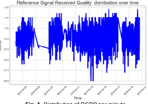
relative distance from serving cell. In the preprocessing and aggregation step all the parameters in the data were aggregated based on time and geospatial information. Locations which had less than 1000 records over different timestamps could not give a defined trend when subject to time series models and were filtered out. Fig. 1,2 and 3 below show the distribution of RSRP, RSRQ and SINR over a period of 20 days.
Fig. 1. Distribution of RSRP per minute
Fig. 2. Distribution of RSRQ per minute
Fig. 3. Distribution of SINR per minute
Fig. 4, 5 and 6 show decomposition of the three measurements. Decomposition is an important technique for time series data exploration. It seeks to construct from an observed time series, several component series, where each of these has a certain characteristic. These are general trend, seasonality and residual. The general trend in the time series is due to fundamental shifts or systemic changes of the process or system it represents. Seasonality is manifested as repetitive periodic deviations after de-trending the data. The residuals are obtained after adjusting the trend and seasonal components are the irregular variations [14], [15]. This was helpful in informing the models to be used for prediction. Since all the three performance measurements were found to have an element of seasonality, the models used had to factor in seasonality.
Fig. 4. Hourly decomposition of RSRP
Fig. 5. Hourly distribution of RSRQ
Fig. 6. Hourly distribution of SINR
4 MACHINE
LEARNING
TECHNIQUES
1390
machine learning models. In the exploratory analysis, it was discovered that performance measurement data exhibited seasonality as shown in figures 4, 5 and 6. This informed the choice of the machine learning models which incorporate temporal features such as seasonality combined with temporal correlations in sub seasonal time scales. Three machine learning models were explored, these are: General Additive Models (GAM) GAMs are a blend of generalized linear model and additive models developed by Trevor Hastie and Robert Tibshirani [16]. They seek to maximize the quality of prediction of a dependent variable by estimating specific functions of the predictor variable connected to the predicted variable via a link [17-18]. Prophet, a GAM developed by Facebook which uses a python framework [19] was used. Auto-regressive moving average models (ARMA) ARMA models are very good in capturing trends because autoregression enables the next time values to be predicted based on the prior time values and the moving average concept utilizes dependency between residual errors to forecast values in the next time [14], [20]. In this case Seasonal Autoregressive Integrated moving average (SARIMA) was used to capture the seasonal elements. Deep learningThese are models based on neural networks which are more versatile in automatic learning of temporal dependencies and automatic handling of temporal structures such as trend and seasonality. Recently deep neural networks have been used in several applications such as text mining, fault detection and speech recognition. Deep learning offers high-level abstraction from the data through its architecture that consists of several non-linear layers [14], [15], [21], [23]. Long-term short-term memory (LSTM) is a type of a deep learning model which uses the recurrent neural network and can learn long term dependencies. It was introduced by Hochreiter & Schmidhuber in 1997 [24] and since then it has become a popular method for various deep learning applications [25], [26], [27].
5 RESULTS
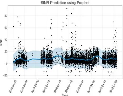
The aim was to predict the performance measurements for the next 60 minutes based on the previous trends for the past 20 days. Three performance measurements were considered which are RSRP, RSRQ and SINR. Figures 7, 8 and 9 show the prediction results for the RSRP, RSRQ and SINR, respectively, achieved using the prophet GAM model. The black dots illustrated in the figures represents the actual measurement readings, the blue line is the prediction with a 60-minute forward rolling window and the light blue thick line is the 95% confidence interval level.
Fig. 7. RSRP Prediction using Prophet
Fig. 8. RSRQ Prediction using Prophet
1391
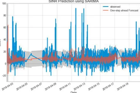
SARIMA model was implemented and the results are as shown in figures 10, 11 and 12. The method of grid search was used for hyperparameter tuning [28], [22]. The blue graph is the actual measurements, the orange graph is the output of the model with a 60-minute forward rolling window and the grey graph is 95% confident interval.
Fig. 10. RSRP Prediction using SARIMA
Fig. 11. RSRQ Prediction using SARIMA
Fig. 12. SINR Prediction using SARIMA
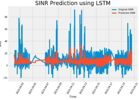
Fig.13, 14 and 15 shows the output of LSTM. The model consisted of an input layer, two stacked LSTM layers having 64 and 32 neurons respectively, and the output layer. The network's weights were optimized using the adaptive moment estimation (Adam) algorithm. Adam algorithm was used since it uses different learning rates for each weight and separately updates them as the training progresses. The learning rate of a weight is updated based on exponentially weighted moving averages of the weight's gradients and the squared gradients [14], [29], [30], [31]. A batch size of 16 was used over the 20 training epochs. The blue graph is the actual measurements, the orange graph is the output of the model with a 60-minute forward rolling window.
Fig. 13. RSRP prediction using LSTM
1392
Fig. 15. SINR prediction using LSTM
6 DISCUSSION
The Dataset was split into train and test data in the ratio of 70:30. K-fold cross validation was used to evaluate the performance of the various models. The dataset was divided into 4 equal subsets and each subset was used to train and test, then an average was done to obtain the results shown in table1 below. Three metrics were used to evaluate the best model; Mean Absolute Error (MAE), Root Mean Square Error (RMSE) and the standard deviation [32].
TABLE I. EVALUATION RESULTS FOR DIFFERENT MODELS
From figures 7,8 and 9 it was evident that prophet GAM was over smoothing the data. This was also evident in the various evaluation metrics. SARIMA offered better results for RSRP and RSRQ with standard deviation of 5.8dB, 6.5dB respectively. However, the SINR had a high standard deviation of 7.4dB. LSTM was found to be the best model with standard deviation of 3.64dB, 4.49dB and 4.46dB for the RSRP, RSRQ and SINR respectively.
7 CONCLUSION AND FUTURE WORK
This paper proposed a temporal prediction approach to radio signal predictions. The best model in this case was LSTM deep learning model with standard deviations of 3.64dB, 4.49dB and 4.46dB for the RSRP, RSRQ and SINR
respectively. These predicted measurements can be used to detect areas that will have coverage or quality issues and actions taken to avert. Predictions for a longer duration can give insights to future base station planning. Future enhancement to this work includes application of a big data framework to analyze massive data coming from the entire network for a longer duration.
ACKNOWLEDGMENT
The authors wish to thank the Pan African University Institute for Basic Sciences, Technology and Innovation (PAUISTI) for their support towards enabling the realization of this research work.
REFERENCES
[1] Elham Jamalian and Rahim Foukerdi, "A Hybrid Data Mining Method for Customer Churn Prediction," Engineering, Technology & Applied Science Research, vol. 8, no. 3, pp. 2991-2997, 2018.
[2] Wickell, Andreas, "Evaluation of statistical models in simulations of 3G and 4G networks," Stockholm, Sweden, 2013.
[3] Johan Johansson, Wuri A. Hapsari, Sean Kelley and Gyula Bodog, "Minimization of Drive Tests in 3GPP Release 11," Technological Advances in LTE Advanced, p. 8, 2012.
[4] Ying He, Fei Richard Yu, Nan Zhao, Hongxi Yin Haipeng Yao and Robert C. Qiu, "Big Data Analytics in Mobile Cellular Networks," IEEE Access, vol. 4, no. 1, pp. 1985 - 1996, 2016. [5] Ejdar Bastug, Mehdi Bennis, Engin Zeydan, Manhal Abdel
Kader, Ilyas Alper Karatepe, Ahmet Salih Er, Mérouane Debbah, "Big data meets telcos: A proactive caching perspective," IEEE Journal of Communications and Networks, vol. 17, no. 6, pp. 549 - 557, 2015.
[6] Mirza Golam Kibria et al, "Big Data Analytics, Machine Learning and Artificial Intelligence in Next-Generation Wireless Networks," IEEE Access, vol. 6, pp. 32328 - 32338, 2018.
[7] Xiaoyong Cheng, "Field strength prediction of mobile communication network based on GIS," Geo-spatial Information Science, vol. 15, no. 3, pp. 199-206, 2012.
[8] Pete Bernardin, "PREDICTING AND VERIFYING CELLULAR NETWORK COVERAGE," Texas Wireless Symposium 2005, vol. 6, no. 1, pp. 11-15, 2005.
[9] Kanagalu Manoj, Pete Bemardin and Lakshman Tamil, "Coverage Prediction for Cellular Networks from Limited Signal Strength Measurements," Ninth IEEE International Symposium on Personal, Indoor and Mobile Radio Communications (Cat. No.98TH8361), pp. 1147-1151, 1998.
[10] Jingming Li, Guoru Ding, Xiaofei Zhang, Qihui Wu, "Recent Advances in Radio Environment Map: A Survey," Machine Learning and Intelligent Communications, vol. 226, pp. 247-257, 2017.
[11] J. R. a. P. Mähönen, "Machine Learning for performance prediction in mobile cellular Network," IEEE Computational Intelligence Magazine, vol. 13, no. 1, pp. 51-56, 2018.
[12] Ana Galindo-Serrano, Berna Sayrac, Sana Ben Jemaa, Janne Riihijärvi, Petri Mähönen, "Harvesting MDT data: Radio environment maps for coverage analysis in cellular networks," 8th International Conference on Cognitive Radio Oriented Wireless Networks, pp. 37-42, 2013.
1393
Vehicular Technology Conference (VTC-Fall), 2018.
[14] Dr. Avishek Pal and Dr. PKS Prakash, Practical Time Series Analysis, Birmingham: Packt Publishing Ltd., 2017.
[15] Rob J Hyndman and George Athanasopoulos, Forecasting: Principles and Practice, Melbourne: Springer, 2018.
[16] T.J. Hastie, R.J. Tibshirani, Generalized Additive Models, Boca Raton: Chapman and Hall/ CRC, 1990.
[17] Thomas W. Yee, Vector Generalized Linear and Additive Models: With an Implementation in R, New York: Springer, 2015. [18] Alain F. Zuur, A Beginner's Guide to Generalized Additive
Models with R, Newburgh: Highland Statistics Limited, 2012. [19] Michael Su, "Prophet Documentation: Release 0.1.0,"
Facebook, 2014.
[20] Mark Pickup, Introduction to Time Series Analysis, Thousand Oaks: Sage publications INC, 2015.
[21] Latifa Belhaj Salah and Fathi Fourati, "Systems Modeling Using Deep Elman Neural Network," Engineering, Technology & Applied Science Research, vol. 9, no. 2, pp. 3881-3886, 2019. [22] Jason Brownlee, Deep Learning for Time Series Forecasting
Predict the Future with MLPs, CNNs and LSTMs in Python, 2019.
[23] Nigel Da Costa Lewis, Deep Time Series Forecasting with Python: An Intuitive Introduction to Deep Learning for Applied Time Series Modeling, Scotts Valley: CreateSpace Independent Publishing Platform, 2016.
[24] Sepp Hochreiter and Jurgen Schmidhuber, "LONG SHORT-TERM MEMORY," Neural Computation, vol. 9, no. 8, pp. 1735-1780, 1997.
[25] Fazle Karim, Somshubra Majumdar, Houshang Darabi, Shun Chen., "LSTM Fully Convolutional Networks for Time Series Classification," IEEE Access, vol. 6, pp. 1662 - 1669, 2017. [26] Yuxiu Hua, Zhifeng Zhao, Rongpeng Li, Xianfu Chen, Zhiming
Liu, Honggang Zhang, "Deep Learning with Long Short-Term Memory for Time Series Prediction," IEEE Communications Magazine, vol. 57, no. 6, pp. 114 - 119, 2019.
[27] Felix A. Gers, Douglas Eck and Jürgen Schmidhuber, "Applying LSTM to Time Series Predictable through Time-Window Approaches," International Conference on Artificial Neural Networks, pp. 669-676, 2001.
[28] James Bergstra and Yoshua Bengoi, "Random Search for Hyper-Parameter Optimization," Journal of Machine Learning Research, vol. 13, pp. 281-305, 2012.
[29] Ian Goodfellow, Yoshua Bengoi and Aaron Courville, Deep Learning, Cambridge, Massachusetts: MIT Press, 2016. [30] Leszek Rutkowski, Ryszard Tadeusiewicz, Lofti A. Zadeh, Jacek
M. Zurada, Artificial intelligence and soft computing, Gewerbestrasse, Switzerland: Springer, 2017.
[31] Larry Medsker, Lakhmi C. Jain, Reccurrent Neural networks Design and Applications, Boca Raton: CRC Press, 1999. [32] Jeonghee Yi, Ye Chen, Jie Li, Swaraj Sett, Tak W. Yan,