Sea surface salinity reconstruction as seen with foraminifera shells: Methods and cases studies

c

EDP Sciences, 2009

DOI: 10.1140/epjconf/e2009-00919-6

P

HYSICAL

J

OURNAL

CONFERENCES

Sea surface salinity reconstruction as seen with

foraminifera shells: Methods and cases studies

B. Malaiz´e and T. Caley

Universit´e Bordeaux 1, UMR 5805 EPOC, Avenue des Facult´es, 33405 Talence, France

Abstract. Reconstruction of past salinities in surface oceans (SSS) can be done by measuring the isotopic composition of foraminifera shells found in the deep sea sediments. The proportion of heavy oxygen isotopes (18_{O) in the calcite of} these shells depend on the temperature and the isotopic oxygen composition of the surrounded waters (δ18_{Osw), this latter parameter depending on the water} salinity. Mainly two equations allows to reconstructed past SSS, one estimating past temperature variations and the other one changes in the δ18_{Osw through} time. Uncertainties linked with these calculation can be important, and therefore quantitative reconstructions need to be taken with cautions. For some specific cases, uncertainties on temperature andδ18_{Osw estimations can be reduced. For} such cases, salinity reconstructions showing amplitude changes higher than 1 per mil can be considered as significative.

1 Introduction

The role of salinity in oceanography is crucial: It plays an important part in the hydrography, i.e. intensities and directions of major current. As a main parameter in the oceanographic engine, it also contributes to heat transfert throughout ocean circulation, and therefore to regional and global climate changes.

To reconstruct past oceanographic conditions, scientists need to gather a huge compilation of data set (oceanic temperatures and salinities) over a long period of time and covering major parts of worldwide oceans. Furthermore, quantitative reconstructions of oceanic parameters are needed as inputs for oceanographic or climatic models. Some sea sediments displays interesting geologic archives, as long as its sedimentation process has not been disturbed, i.e. without any time gap or physical disruption (such as turbiditic flows on continental shelf or biotur-bation). Microfossils of past oceanic life can be found in these archives, and their assem-blages oftenly give indications on the conditions in which they developed, as for example mean sea surface temperatures (hereafter SST). Only few geological archives are known to be dir-ectly related to sea surface salinities (hereafter SSS), and therefore, some indirect method, based on foraminifera microfossils, have been developed to reconstruct past SSS. As long as some foraminifera species have specific living requirements, studies have investigated past SSS reconstructions based on foraminiferal abundance data. The use of Artificial Neural Net-work, or Modern Analog Technique, have led to the conclusion that such estimations were unrealistic [1], and can’t be considered as quantitative. Therefore, scientists turned their atten-tion to geochemical analysis of foraminifera species, which could lead to quantitative estimaatten-tions of SSS.

The aim of this paper is to present an overview of past sea surface salinities reconstructions through the chemistry of foraminifera microfossils, to estimate uncertainties of such paleo-records, and to discuss wether it can be used as quantitative parameters or not.

δ

_Oc

_δ

Osw

SST

SSS

Ice Volume P/E and discharge

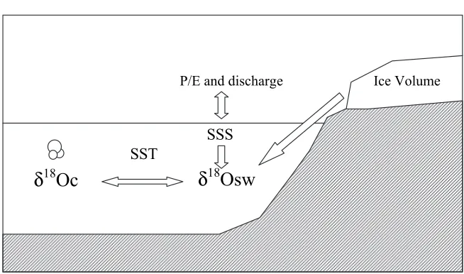
Fig. 1.Main parameters influencing the isotopic composition of planktonic foraminifera shells (δ18Oc): Sea surface temperature (SST) and the isotopic composition of the surrounded waters (δ18Osw). This last parameter is also dependant on sea surface salinity (SSS), linked with the evaporation-precipitation balance (P/E) and with the volume of continental ice sheets (depleted in heavy isotopes).

2 Stable isotopes fractionation in foraminifera shells

2.1 Today

Marine invertebrates such as foraminifera are building exoskeletons made of calcium carbon-ate to protect themselves from predators. Isotopic fractionations are taking place during this process, depending on both the proportion of stable isotopes available in the waters surrounding the foraminifera and the temperature of these waters (Figure 1). Many experimental and theo-retical studies have been held since the middle of last century to understand the incorporation of oxygen isotopes in foraminifera shells.

Epstein et al., in 1953, established a paleotemperature equation, linking the temperature with the isotopic composition of the calcite and of the surrounded waters [2]. Shackleton and Opdyke have adapted this equation in 1973 [2] into the following one:

T = 16.9−4.38(δ18Oc−δ18Osw) + 0.13(δ18Oc−δ18Osw)2 (1)

(δ18Oc is the isotopic value of the calcite, and δ18Osw the isotopic composition of the sea water).

This relationship holds only if foraminifera deposit their shells in isotopic equilibrium with their growth medium. An overview of several oceanic sites revealed that only few species fits these requirements. Meanwhile, some quantitative temperature reconstructions seems to be possible.

This equation underlines the double dependance of the δ18Oc of the foraminiferal shell with temperature changes together with the marine isotopic composition changesδ18Osw. We have one equation with two unknowned. To complicate the solving,δ18Osw is also dependent on salinity changes. A first overview of experimental measurements, made in 1965, following a series of observations made during oceanic cruises over different oceans (top cores), allows Craig and Gordon to established a first salinity–water isotope relationship (Figure 2) [4]:

δ18_{Osw = 0.66 SSS−23.5. (2)}

2.0

1.5

1.0

0.5

0.0

-0.5

-1.0

-1.5

39 38 37 36 35 34 33 32 31

Craig and Gordon, 1965

GEOSECS (Östlund et al., 1987)

Arabian Sea (Delaygue et al., 2001)

δ

18

O ( ‰

)

SSS ( ‰ )

Fig. 2.Differentδ18Osw-salinity relationships deduced from two different data sets of the worldwide oceans [4] from GEOSECS cruises [24], and from modeled output gathered with observed data from the Arabian Sea [36]. Data compiled by Gavin Schmidt [25],http://data.giss.nasa.gov/o18data/.

To conclude, the δ18Oc of a monospecific species of foraminifera is directly dependent on the temperature, but also undirectly dependent on the salinity which follows the δ18Osw. Equations (1) and (2) were build using specific foraminifera species, within a certain range of temperature and salinity. They could be applied only for some specific situation.

Within these requirements and according to equations (1) and (2), salinity reconstruction can be done using the estimations of two different oceanic parameters: Sea surface temperatures andδ18Osw values. This latter term can be evaluated with the resolution of equation (1), with temperatures estimations andδ18O of the calcite of the foraminifera shell.

δ18_{Osw =δ}18_{Oc + 0.27−5(4.38−}√_(4.382_{−0.4(16.9−SST)) (3)}

(Factor 0.27 is added for calibration against international standard).

In fine, to calculate SSS, we are bounded to a system with two equations, (2)+(3), and two unknowned parameters (δ18Osw and SST). For today’s measurements, no other equations are needed.

2.2 Reconstruction of SSS in the past

Today’s observations are questionned to be applyed in the past. Emiliani et al. were the first to published an isotopic curve extracted from benthic and planctonic foraminifera in deep sea cores, which they interpreted in terms of past variations of climatic parameters [5]. Most of this signal has been interpreted in terms of paleotemperatures, but not much in terms of paleosalinities.

To estimate past SSS, three terms need to be taken into account:

1. Modification of global salinity due to global changes in continental ice sheet volume (i.e.

2. Modification of the local salinity due to regional changes in the hydrographic balance (linked with local SST)

3. Modification of theδ18Osw due to global changes in continental ice sheet. During deglacia-tion times, fresh water discharges coming from the melting of continental ice sheet invade oceans, changing their salinity and, as a consequence, their isotopic compositions.

The last two terms are contributing to changes in the local/global SSS (i.e. ∆SSS_Loc-Glob).

Adding these changes to present SSS allows to evaluate past SSS.

SSS_Past= SSS_Present+∆SSS_G-IG+∆SSSLoc-Glob.

To calculate changes in SSS on a global and local scale (∆SSS_Loc-Glob), changes in temperatures

andδ18Osw in the past need to be estimated.

If past variations in SST are easy to link with climatic changes, modification of the isotopic composition of sea waters might be a less straightforward reasoning.

On a global scale, the building of huge ice caps on the continent during glacial periods leads to an enrichment of the worldwide oceans in heavy18O isotopes (Figure 1). This enrichment is due to thermodynamic fractionation processes taking place during different stages of the hydrological cycle. Heavy isotopes concentrate more in densier phases, contributes to a stronger concentration of light isotopes in the continental ice, and, as a consequence, to a stronger concentration of heavier isotopes in oceans.

Glacial-interglacial changes lead to global salinities changes in the worldwide oceans (figure 1). As continental ice sheet are made with fresh water, the consequence is an increase of salinity in the ocean when entering a glacial period. If equation (2) stays valid in the past, the isotopic composition of the ocean should have changed in response to these salinity changes. In addition to these artefact due to global effects (directly onδ18Osw and SSS), local changes could affect also specifically some part of the ocean. For example, climatic change could lead to some modifications in the balance between evaporation and precipitation over a studied area. Such changes might have contributed to modify locally salinity concentrations, and therefore the isotopic composition of the surface sea waters.

The problem is that no geological archive has directly recorded past δ18Osw values, on a local neither a global scale. One way to solve this apparent problem is to distinguish the planktonic isotopic record from the benthic isotopic record. Indeed, for some remoted and deep environments, benthic foraminifera are surrounded by waters for which temperature and salinity changes can be constrained. For these environments, for deep part of the Pacific ocean for example, some isotopic studies have focused on the estimation of deep water temperature changes and their imprint on the benthic isotopic signal. Adding some calibration to sea level changes, estimations ofδ18Osw changes through glacial-interglacial periods can be done. Some scientists had compiled several benthic records from different deep oceanic areas where such estimations can be done. Some reference stacks of benthic records have been published, and linked to global sea level changes (Figure 3) [6–10].

Once these δ18Osw changes due to global effect have been estimated, δ18Osw changes due to local effect (past and present) need to be estimates. One way to solve this problem is to resolve equation (3), requiring estimation of past temperatures.

Difficulties to apply reliationships (3) and (2) in the past are numerous. For example, isotopic measurements need to be done on a well studied monospecific species, constantly present in time (no evolution) and defined to be in isotopic equilibrium (or showing a constant difference) with the standard water composition. Secondly, the reconstructed temperatures and salinities need to be within the range defined by equations.

3 SST estimations: Solving equation (3)

-180 -160 -140 -120 -100 -80 -60 -40 -20 0 20 40 60

0 50 100 150 200 250 300 350 400 450

Age, ka RS L , m -1,45 -0,95 -0,45 0,05 S h ac kl e to n se a l e v e l, ‰

Coral reef estimates Rohling [1998]

Waelbroeck et al. (submitted) error -, m

error +, m Shackleton [2000]

Fig. 3.Sea level reconstruction and consequent globalδ18_{Osw changes through time [6–8].}

‘transfert function’ applied since then to other proxies. The purpose is to compare present-day distribution of foraminifera to oceanic temperature distribution, and to extract the most repre-sentative species of specific temperature intervals. Some other technics have been developed since this first study [12], as the Modern Analogue Technic (MAT) for example. Application of these reconstructions to the last glacial maximum climatic conditions led to different maps showing SST distributions for this specific time period, as for example the CLIMAP project [13], or the more recent MARGO project [14]. The best reconstructions are able to reproduce temperature within a +/−1.3◦C uncertainties intervals [12].

Another way to reconstruct surface temperature is to look at today’s distribution of the difference between δ18Osw and δ18Ocalcite, and then to apply equation (1). Duplessy et al. presented the first SSS reconstruction, mixing previous transfert fonction SST estimates together with statistical analysis of isotopic measurements made on 83 core tops from North Atlantic and Southern Oceans [15]. The authors pointed out different calibrations of calcifi-cation temperature, depending on each studied species. For G. bulloides, a 1◦C difference is observed between summer SST and the calcification temperature, although 2.5◦C difference is due for N. pachyderma. This study underlines one main difficulty in such reconstruction, for which the calcification temperature depends on the foraminifera species.

Recently, geochemistry development has proposed a new technic to estimate SST via individual foraminifera species analysis, removing uncertainties in equation (1) due toδ18Osw changes through time, linked to either global or local changes. Theoretically, Mg2+ alkaline ele-ment can replace Ca2+element in the rhombohederal structure of the calcite. Thermodynamic predictions, along with experimental observations, have demonstrated a major temperature control on the distribution coefficient [16–20]. For foraminifera species, some calibrations were needed to estimate the biological effect on this partitioning. Culture studies, as well as sediment trap sample studies, led to a similar exponential dependence calibration for different planktonic species [21]:

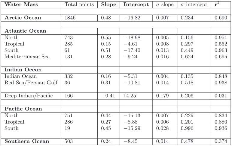
Table 1. Adapted from LeGrande and Schmidt 2006.

Water Mass Total points Slope Intercept σslope σintercept r2

Arctic Ocean 1846 0.48 −16.82 0.007 0.234 0.690

Atlantic Ocean

North 743 0.55 −18.98 0.005 0.156 0.951

Tropical 285 0.15 −4.61 0.008 0.297 0.552

South 61 0.51 −17.40 0.013 0.449 0.963

Mediterranean Sea 131 0.28 −9.24 0.016 0.624 0.695

Indian Ocean

Indian Ocean 332 0.16 −5.31 0.004 0.135 0.848

Red Sea/Persian Gulf 36 0.31 −10.81 0.014 0.518 0.938 Deep Indian/Pacific 166 −0.41 14.25 0.179 6.206 0.031 Pacific Ocean

North 751 0.44 −15.13 0.007 0.229 0.834

Tropical 286 0.27 −8.88 0.006 0.201 0.880

South 19 0.45 −15.29 0.028 0.996 0.936

Southern Ocean 503 0.24 −8.45 0.014 0.478 0.374

A and B are two constants, defined for each foraminifera species and for different size [22]. As long as some discrepancies has been observed within the same species, Mg/Ca measurements needs to be done on the same morphotype and within the same size fraction (to avoid different partitioning linked to juvenil foraminifera having a faster calcification than the older ones) [23]. These precautions need to be taken also for isotopic measurements on foraminifera species

New studies are on their way to investigate other potential biais to this technic, linked with some dissolution effect on the Mg/Ca incorporation, or also some influence of post-crystallization.

At present, taking all these observations into account, uncertainties linked to these recon-structions can be estimated at best around +/−1.2◦C.

4 SSS-

δ

_{O ocean relationship: Solving equation (2)}

Global variations of the isotopic composition of sea water, δ18Osw, can be estimated thanks to constructed stack of benthic foraminifera δ18O (see end of section 2.2). Local variations of

δ18_{Osw can be estimate with equation (3), measuringδ}18_{Oc of a specific foraminifera species}

and having estimated past SST changes (section 3).

Once global and local variations in δ18Osw have been estimated, past SSS values can be calculated using equation (2). The main problem is that this relationship presents different slopes and intercept values.

one. On a regional scale, taking the tropical band as an example, fresh water inputs via precip-itation could happen close to areas of evaporation, and therefore isotopic values of rainfall and evaporation waters can be very similar. As a consequence, slopes are shallower than the ones in mid or higher latitude. On a temporal scale, seasonnal events such as discharge of fresh water in coastal areas close to a river mouth, or sea ice melwater signals at high latitudes, can influence the salinity-δ18Osw relationship. On a longer time scale, some studies have demonstrated that the hydrologic cycle, together with the high latitude end-member of precipitation, have obvi-ously changed in the past, as for example during the last glacial maximum [27]. Model results have shown that for smallδ18Osw changes, there were no correlation between the spatial and the temporal gradient [25]. Important uncertainties still remain on the amplitude of changes in the linear relationship through time.

On a regional point of view, the correlation coefficient (r2), linked to each of these local linear least squareδ18O-SSS relationship, goes from very poor value (0.031 for the deep Pacific/Indian oceans) to very high values (0.951 for the North Atlantic ocean)(Table 1). As a consequence, confidence in the results of equation (2) depends on the area where the salinity reconstruction takes place.

Within consequent (but still acceptable) uncertainties, quantitative SSS reconstructions can be done and trusted for areas with a high correlation factor, such as for the Artic ocean, North and South Atlantic Ocean, Red sea/Persian Gulf, amongst others. For other areas, as the general tropic areas, for which slopes of theδ18O-SSS relationship are shallower than for other latitudes (tropical Atlantic and Pacific), errors are larger [25], and quantitative SSS reconstructions need to be taken with caution.

5 Uncertainties: What to use as a more accurate proxy?

As seen in section 3 and 4, uncertainties inherent in quantitative SSS reconstructions can be linked to three different steps in the calculation:

1. The accuracy of SST estimations

2. Global δ18Osw and salinity changes linked to glacial-interglacial continental ice volume changes.

3. Temporal and spatial decrepancies of theδ18Osw-SSS relationship (equation (2)).

For the temperatures reconstructions, main uncertainties are between +/−1.9◦C and +/−1◦C, depending on the used method (Table 2) [25]. The most recent studies benefit high resolution or geochemistry developments which drag most of the main temperature uncertainties closer to a best value of +/−1◦C. Transcript into an isotopic scale, using equation (3), the deduced error onδ18Osw estimation is between +/−0.52 and +/−0.23 per mil.

The source of uncertainty due to glacial-interglacial changes on a global scale has been constrained in the past by many studies, using multiproxy approach and models, which helped to reduce the error bars [7, 8]. It has reached a mean value for the Last Glacial Maximum (LGM) of about 1.1 +/−0.1 per mil forδ18Osw, and 1 +/−0.05 per mil for the salinity [25]. Maximum uncertainties are found for period of rapid ice volume changes, as long as it is difficult to estimate the propagation of surface changes down to the deep ocean. It is supposed to be well mixed for period above 1,000 years [25].

For the δ18Osw-SSS relationship accuracy, the question of its permanence in time is still unsolved. Again, time periods covering rapid ice volume changes, such as deglaciations, present strongest uncertainties than for rather stable climatic periods. For spatial scattering of slopes and intercept numbers, compilation of studied areas are now available and presents, for most linear relationships, uncertainties, confidence intervals and/or correlation factor (table 1) [26]. Estimations of global errors due to these uncertainties range from 1.1 to 0.8 per mil. For tropical area, the range is higher, going from 1.8 to 1.2 per mil uncertainty [25], except for some well defined restricted areas.

Considering all these uncertainties, does paleosalinity reconstruction hold tight?

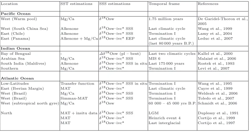
Table 2.Compilation of different case studies focusing on Sea surface salinity reconstruction. For SST estimations, MAT stands for Modern Analog Technic. For SSS estimations,δ18_{Osw–ivc* corresponds} to the residual δ18_{Osw signal corrected from the global ice volume (icv), and SSS underlines that} quantitative salinity reconstructions are presented in the references.

Location SST estimations SSS estimations Temporal frame References

Pacific Ocean

West (Warm pool) Mg/Ca δ18Osw 1.75 million years De Garidel-Thoron et al., 2005

West (South China Sea) Alkenone δ18Osw–ivc* SSS Last climatic cycle Wang et al., 1999 East (Chile) Alkenone δ18Osw–ivc* SSS Termination I Lamy et al., 2004 East (Panama) Alkenone + Mg/Caδ18Osw–ivc* EEP Last climatic cycle Leduc et al., 2007

(last 80 000 years B.P.)

Indian Ocean

Bay of Bengual - ∆δ18Osw (pl – bent) Last two climatic cycles Kallel et al., 2000

Arabian Sea Mg/Ca δ18Osw–ivc* SSS MIS 6 Malaiz´e et al., 2006

South India (Maldives) Alkenone δ18Osw–ivc* SSS in situ Last 175 000 years Rostek et al., 1993

Southern Mg/Ca δ18Osw–ivc* Termination I Levi et al., 2007

Atlantic Ocean

Low-Latitudes Transfer function δ18Osw–ivc* SSS in situ Termination I Wang et al., 1995 East (Iberian Margin) MAT δ18Osw–ivc* Last climatic cycle Cayre et al., 1999 West (Brasil) Mg/Ca δ18Osw–ivc* SSS Termination I Weldeab et al., 2006 West (Brasil) Simmax-MAT δ18Osw–ivc* SSS Termination I Toledo et al., 2007 West (subtropical north gyre) Mg/Ca δ18Osw 60 000 – 45 000 yrs B.P. Schmidt et al., 2006

North MAT + insitu dataδ18Osw–ivc* SSS LGM Duplessy et al., 1991 MAT δ18Osw–ivc* Heinrich event 4 Cortijo et al., 1999 MAT δ18Osw–ivc* Last interglacial Cortijo et al., 1997

can’t be reasonably taken as boundary condition for ocean and/or climate models. Netherthe-less, it can be considered as an estimation of changes on a qualitative point of view.

To avoid the most important uncertainty, linked with temporal and spatial decrepancies of the δ18Osw-SSS relationship, good qualitative SSS reconstruction can be done by avoiding the final step in the SSS calculation. A simple signal, obtained with a good SST estimation (equation (3)) (better in situ proxies such as Mg/Ca ratios), together with a good estimation of a global glacial-interglacial change estimation, lead to a residualδ18Osw which represents fairly well past SSS variations, with uncertainties within +/−0.5 per mil. In other words, amplitude changes above 1 per mil in the residual δ18Osw signal can be considered as true qualitative change in SSS.

6 Case studies

According to uncertainty considerations, past SSS reconstructions have been done since the last 17 years, presenting qualitative and/or quantitative results (Table 2). Different approaches, i.e. residualδ18Osw, corrected or not from ice volume changes (ivc), or calculated SSS, depend on the accuracy of each steps in the calculation.

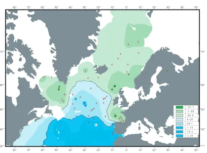
Fig. 4. Reconstruction of summer sea surface salinity for the North Atlantic Ocean during the last glacial maximum (expressed as S-35). Data sets from [15]. Salinity fronts interpolated with Arcview software (acknowledgement to F. Eynaud).

same reconstruction technic has revealed paleosalinities changes of about 1 per mil for such abrupt climatic changes [28–30]. This range in salinity changes holds the limits of confidence defined previously. These quantitative paleosalinity data sets have been used as boundary con-ditions for several ocean model runs, to investigate surface hydrological changes during Heinrich events and the LGM [31, 32].

Two recent studies have focused on specific low latitude areas of the west Atlantic ocean. For both studies, SST estimations are based on Mg/Ca measurements on the same foraminifera species used for isotopic measurements. As described previously, such in situ proxies help to reduce uncertainties on SST. For the subtropical North Atlantic gyre, Schmidt et al. presents

δ18_{Osw record for some of the most drastic climatic episodes covering the last glacial period,}

known as Dansgaard-Oeschger events [33]. Millenial-scale surface-salinity enrichments of about 0.7 to 1.5 per mil are detected for two stadials (cold) events at around 48 000 and 57 000 yrs B.P.. These estimations are using the assumption that present day δ18Osw-SSS relationship was still valid in the past, which should be taken with care. The author suggests that the slope might have been steeper during glacial time, reducing the reconstruct salinity values below 1 per mil unit [33]. Another study has focused on the brasilian margin, and proposed quanti-tative SSS reconstructions for the last deglaciation [34]. On a quantiquanti-tative point of view, two high salinity imprints are recorded for cold periods such as the Younger Dryas period and the Heinrich 1 events, which amplitude are above 1 per mil. Once again, application of the present dayδ18Osw-SSS relationship to the past cast some doubt about the accuracy of such reconstruction. Meanwhile, both reconstructions give probably trustfull qualitative pattern of SSS changes in this area during millenial scale climatic changes.

δ18_{Osw reconstructions in order to estimate past changes in the surface salinity. Only one}

ven-tures to show quantitative SSS values, for the imprints of the last deglaciation on the Chilean margin [35]. For this study, alkenones measurements have been done to estimate SST changes. This alkenone technic is based on measurements done on coccolithophorid chemical remains. Although SST reconstructions using this technic have been thoroughly validated in the past, its application to our SSS reconstruction can still be in abeyance as long as coccolithophorids species might not have the same environmental requirements as foraminifera species. Mean-while, huge decrease in calculated salinities is recorded between 17.8 to 15.8 kyr B.P., with a amplitude of 5 per mil. As long as this salinity change equals 5 times the acceptable uncertainty range (1 per mil), one can consider this imprint to be a realistic signal, linked with the dynamic of the Patagonian Ice sheet [35].

For the Indian ocean, the main problem lies in the weak δ18Osw-SSS relationship. The slope is around 0.20, but with a large standard deviation due to a wide scattering of data points (Figure 2) [36]. As a consequence, except for some well defined areas, quantitative reconstructions are difficult to obtained. Most of the studies present aδ18Osw signal as a proxy for past SSS [37, 38]. To reach good confidence in the quantitative reconstruction, precisions need to be obtained for theδ18Osw-SSS relationship. As seen previously, the correlation factor is quite correct for the Red Sea/Persian Gulf, and can be taken for such calculations. Trusting this good confidence in theδ18Osw-SSS relationship, Malaiz´e et al. tempted to calculate quan-titative changes in SSS during the penultimate glacial period (at around 175 000 years B.P.), a time interval knowned to harbour some strong monsoonal imprints. Rapid decrease of salinity of about 1 per mil is recorded near the Socotran Island during this time, and is linked with fresh water input in the surface ocean, in respons to strong monsoonal rainfall [39]. Anomalies in a

δ18_{Osw residual signal from a marine record taken in the gulf of Bengual, for the same period}

of time, have been also interpreted as a low salinity imprint due to strong indian monsoon [37].

7 Conclusions

As long as no geological archives are knowned to directly record sea surface parameters, sci-entists are bounded to use indirect method to reconstruct past Sea Surface Salinities. Geo-chemistry of foraminifera shell has revealed a strong potential for this purpose. The δ18Oc of the calcitic shell depends on the temperature and on the δ18Osw of the surrounded waters, itself depending on changes in the continental ice sheets volume and on salinity changes. Some experimental observations have led to the development of mathematical relationship between all these parameters (equations (1) and (2)).

To estimate past SSS, three parameters need to be known:δ18Oc, SST, and∆δ18Osw, which could be due to local and global phenomenom (such as ice volume changes). The isotopic com-position of the calcite is directly measured. Analytical precision is given for each measurements. To estimate past SST, several methods have been developed, from faunistic assemblages to geo-chemical studies (Mg/Ca proportion in the shell). The best uncertainty on this parameter can be estimate around 1◦C. The global part ofδ18Osw changes can be estimate with references record, linked with an uncertainty of about +/−0.1 per mil. The local part ofδ18Osw changes can be calculated with equation (1), major uncertainties depending on SST error bars. The main error on quantitative SSS reconstruction is linked with the last step of the calculation, i.e. with the δ18Osw-SSS relationship, which presents a wide range of slopes and scattering of data points. For some specific oceanic areas, uncertainties are to high to allowed quantitative reconstructions, and the final step in the calculation must be avoided. For judicious oceanic areas, quantitative reconstructions can be tested. If the amplitude in SSS changes is below 1 per mil, SSS estimations should be taken with caution.

References

1. T. Wolff, B. Grieger, W. Hale, A. D¨urkoop, S. Mulitza, J. P¨atzold, G. Wefer, Use of Proxies in

Paleoceanography: Examples from the South Atlantic(Springer, Heidelberg, 1999)

2. S. Epstein, R. Buchsbaum, H.A. Lowenstam, H. Urey, Geol. Soc. Am. Bull.64, 1315 (1953) 3. N.J. Shackleton, N. Opdyke, Quat. Res.3, 39 (1973)

4. H. Craig, L.I. Gordon,Stable isotopes in Oceanographic Studies and Paleotemperatures(Tongiorgi, CNR Pisa, 1965)

5. Emiliani, J. Geol.63, 538 (1955)

6. E.J. Rohling, M. Fento, F.J. Jorissen, P. Bertrand, G. Ganssen, J.P. Caulet, Nature394, 162 (1998) 7. N.J. Shackleton, M.A. Hall, E. Vincent, Paleoceanogr.15, 565 (2000)

8. C. Waelbroeck, L. Labeyrie, E. Michel, J.C. Duplessy, J.F. McManus, K. Lambeck, E. Balbon, M. Labracherie, Quat. Sci. Rev.21, 295 (2002)

9. L.E. Lisiecki, M.E. Raymo, Paleoceanogr.20, 1003 (2005)

10. R.S. Bintanja, W. van de Wal, J. Oerlemans, Nature437, 125 (2005)doi:10.1038/nature03975 11. J. Imbrie, N.G. Kipp,The late Cenozoic glacial ages (Yale University Press, 1971)

12. J. Guiot, A. deVernal,Proxies in the Late Cenozoic Paleoceanography (Geotop Qu´ebec, Canada, Elsevier, 2007)

13. CLIMAP Members, Science191, 1131 (1976) 14. Kucera, et al., Quat. Sci. Rev.24, 951 (2005)

15. J.C. Duplessy, L. Labeyrie, A. Juillet-Leclerc, F. Maitre, J. Duprat, M. Sarnthein, Oceanol. Acta 14, 311 (1991)

16. Y. Rosenthal, E.A. Boyle, N. Slowey, Geochim. Cosmochem. Acta61, 3633 (1997) 17. D.W. Lea, T.A. Mashiotta, H.J. Spero, Geochim. Cosmochem. Acta63, 2369 (1999) 18. E.A. Burton, L.M. Walter, Geochim. Cosmochem. Acta55, 775 (1991)

19. A. Mucci, Geochim. Cosmochem. Acta,51, 1977 (1987)

20. T. Oomori, H. Kameshima, Y. Maezato, Y. Kitano, Marine Chem.20, 327 (1987) 21. P. Anand, H. Elderfield, M.H. Conte, Paleoceanogr.18, 15 (2003)

22. Y. Rosenthal,Proxies in the Late Cenozoic Paleoceanography(Geotop Qu´ebec, Canada, Elsevier, 2007)

23. H. Elderfield, M. Vautravers, M. Cooper, Geochem. Geophys. Geosyst.3, 13 (2002) 24. H.G. Ostlund, G. Possnert, J.H. Swift, J. Geophys. Res.92, 3769 (1987)

25. G.A. Schmidt, Paleoceanogr.14, 422 (1999)http://data.giss.nasa.gov/o18data/ 26. A.N. LeGrande, G.A. Schmidt, Geophys. Res. Lett.33, L12604 (2006)

27. E.J. Rohling, G.R. Bigg, J. Geophys. Res.103, 1307 (1998)

28. E. Cortijo, J.C. Duplessy, L. Labeyrie, H. Leclaire, J. Duprat, T.C.E. van Weering, Nature372, 446 (1994)

29. E. Cortijo, L. Labeyrie, L. Vidal, M. Vautravers, M. Chapman, J.C. Duplessy, M. Elliot, M. Arnold, J.L. Turon, G. Auffret, Earth Planet. Sci. Lett.146, 29 (1997)

30. E. Cortijo, S. Lehman, L. Keigwin, M. Chapman, D. Paillard, L. Labeyrie, Paleoceanogr.14, 23 (1999)

31. D. Paillard, E. Cortijo, Paleoceaogr.14, 716 (1999)

32. A.M.E. Winguth, D. Archer, J.C. Duplessy, E. Maier-Reimer, U. Mikolajewicz, Paleoceanogr.14, 304 (1999)

33. M.W. Schmidt, M. Vautravers, H.J. Spero, Nature443, 561 (2006)

34. S. Weldeab, R.R. Schneider, M. K¨olling, Earth Planet. Sci. Lett.241, 699 (2006)

35. F. Lamy, J. Kaiser, U. Ninnemann, D. Hebbeln, H.W. Arz, J. Stoner, Science304, 1959 (2004) 36. G. Delaygue, E. Bard, C. Roillon, J. Jouzel, M. Stievenard, J.C. Duplessy, G. Ganssen, J. Geophys.

Res.106, 4565 (2001)

37. N. Kallel, J.C. Duplessy, L. Labeyrie, M. Fontugne, M. Paterne, M. Montacer, Palaeogeogr. Plalaeoclim. Palaeoecol.157, 45 (2000)

38. C. Levi, L. Labeyrie, F. Bassinot, F. Guichard, E. Cortijo, C. Waelbroeck, N. Caillon, J. Duprat, T. de Garidel-Thoron, H. Elderfield, Geochem. Geophys. Geosyst.8(2007)

39. B. Malaiz´e, C. Joly, M.T. V´enec-Peyr´e, F. Bassinot, N. Caillon, K. Charlier, Geochem. Geophys. Geosyst.7(2006)

40. T. de Garidel-Thoron, Y. Rosenthal, F. Bassinot, L. Beaufort, Nature433, 294 (2005)

42. F. Rostek, G. Ruhland, F. Bassinot, P.J. Muller, L. Labeyrie, Y. Lancelot, E. Bard, Nature364, 319 (1993)

43. L. Wang, M. Sarnthein, J.C. Duplessy, H. Erlenkeuser, S. Jung, U. Pflaumann, Paleoceanogr.10, 749 (1995)

44. L. Wang, M. Sarnthein, H. Erlenkeuser, J. Grimatl, P. Grootes, S. Heilig, I. Ivanova, M. Kienast, C. Pelejero, U. Pflaumann, Marine Geol.156, 245 (1999)