TCSC Control of Power System oscillation and Analysis using Eigenvalue Techniques

TCSC Control of Power System oscillation and

Analysis using Eigenvalue Techniques

M.W. Mustafa. MIEEE ,Nuraddeen Magaji, IEEE Student Memberand Z. bint Muda

Universiti Teknologi Malaysia, Department of Power Engineering, Johor Bahru, Malaysia [email protected]

Abstract— TCSC devices are used to improve real power an d eliminate line loses in ac systems. An additional task of TCSC is to increase transmission capacity as result of power oscillation damping. In this paper eigenvalue-based methods for analysis and control of power system oscillations using TCS C have been developed. The characterization of power system oscillations using the eigenvalues and eigenvectors of the state matrix is detailed. Design of power system damping controllers using residue method is addressed for two area four machine systems. The result shows the effectiveness of the method used

Index Term-- TCS C, Power system oscillations, linear models, eigenvalues, eigenvectors, participation factors and residue.

I. INT RODUCT ION

The concept of fle xible ac transmission systems is made possible by the application of high power electronic

devices for power flow and voltage control [l]. In addition

a number o f TCSC devices have already been installed to aid power system dynamics wh ich help to mitigation a lo w frequency oscillations often arise between areas in a large

interconnected power network [2].

Eigenvalue sensitivities are one important outcome of the modal analysis and control of oscillatory behaviour and dynamic stability in power systems. The pioneering work

[3] considers the local oscillation of a single machine by means of a transfer function model. The usually co mple x pattern of oscillations in a large power system can be studied through linear, t ime invariant, state-space models based on the perturbations of the system state variables fro m their nominal values at a specific operating point

Power system oscillations occur due to the lack of damp ing torque at the generators rotors. The oscillation of the generators rotors cause the oscillat ion of other power system variables (bus voltage, bus frequency, transmission lines active and reactive powers, etc.). Po wer system oscillations

are usually in the range between 0.1 and 2 Hz depending on

the number of generators involved in [4]. Loca l oscillations

lie in the upper part of that range and consist of the oscillation of a single generator or a group of generators against the rest of the system. In contrast, inter-area oscillations are in the lower part of the frequency range and comprise the oscillations a mong groups of generators. In addition, power system oscillations exh ibit low da mping compared to oscillations found in other dynamic systems: an oscillation of 10% da mp ing is commonly accepted as well damped. To imp rove the damping of oscillations in power systems, supplementary control la ws can be applied to e xisting devices. These supplementary actions are refe rred to as power oscillation damping (POD) control

This paper revie ws the basic concepts of eigenvalue analysis

eigenvectors, participation factors, residues and

controllability and observability indices will be introduced and illustrated in small scale power systems. This technique has been successfully used in location and tuning of powe r

system stabilizers [5] and FACTS devices.

The application of sensitivity measures to the design of power system da mping (POD) controllers has been applied to TCSC. The design method utilizes the residue approach; this presented approach solves the optima l sitting o f the TCSC device, selection of the proper feedback signals and

the controller design problem [6].

II. LINEAR SYST EM ANALYSIS T OOLS IN POWER SYST EMS

Low frequency electro mechanical oscillations range fro m less than 1 Hz to 3 Hz other than those with

sub-synchronous resonance (SSR) [6,15]. Mu lti-machine powe r

system dynamic behavior in this frequency range is usually e xpressed as a set of non-linear differentia l and algebraic (DA E) equations. The algebraic equations result from th e network powe r ba lance and generator stator current equations. The init ia l operating state of the algebra ic variables such as bus voltages and angles are obtained through a standard power flow solution. The in itia l values of the dynamic variables are obtained by solving the differential equations

A. Eigenvalues, Eigenvectors and Modes

Let us start from the mathe matica l model a dynamic system e xpressed in terms of a system of non-linear d ifferentia l equations:

( , )

xF x t (1)

If th is system of non-linear d iffe rential equations is Linearized around an operating point of interest x=x0, it results in:

( )   x A x t

(2)

A mean ingful solution method of (2) is based on the eigenvalues and eigenvectors of the state matrix A. An

eigenvalue



_i of the state matrix A and the associated right

vi and left wi eigenvectors are defined accord ing to:

i i i

Av





v

In a mat rix with all distinct eigenvalues (not a necessity but it is easier to understand when it is so), all the right eigenvectors and eigenvalues can be expressed as a compact matrix expression



AV VA (3)

Where,

( _{1 2} ... _{n 1 n}, )

V v ,v v v

    



 (4)

International Journal of Engineering & Technology IJET-IJENS Vol:09 No:10 38

Pre-multiplying both sides of (3) by V-1gives

1

V AV    (5)

Asimilar e xpression holds for the left eigenvectors W such

that

WA W (6)

Where

1 2 1

[ t t ... t t t]

n n

W   ,   (7)

Post-multiplying both sides of (6) by W-l, gives

1

 _{ }

WAW (8)

The transformed physical state variables (x) can be put into

modal variables (2) with the help of eigenvector matrices V

and W

x Vz

z Wx



 (9)

In power system lite rature, the right eigenvector matrix v is

known as the mode shape matrix, that is, eigenvector vi is

known as the ithmode shape, corresponding to eigenvalue λi.

The mode shape provides important in formation on the participation of an individual machine or a group of machines in one particular mode.

solution of (2) can be e xpressed in terms of the eigenvalues and eigenvectors of the state matrix as:

i

N t

t T

i i

i

x(t) Ve W x( ) v e [w x( )] 1

0  0





   



 (10)

The analysis of equation (10) allo ws drawing the fo llo wing

conclusions:

i. The system response is the comb ination of the

system response to each of the N modes.

ii. The eigenvalues determine the system stability. A

real positive (negative) eigenvalue determines

e xponentially increasing (decreasing) behavior. A

comple x e igenvalue of positive (negative) real part results in a increasing (decreasing) oscillatory behavior.

iii. The components of the right eigenvector vi

measure the relative activity of each variable in the ith mode.

iv. The components of the left eigenvector wi we ight

the initial conditions in the i-th mode

B. Participation factors

It is natural to suggest that the significant state variables influencing a particular mode are those having larg e entries

corresponding to the right eigenvector of λi. The

participation factor ofthe j-th variable in the k-th mode is defined as the product of the j-th's co mponents of the right

vjkand left wkieigenvectors corresponding to the k-th mode

[7]

jk jk kj

P =W V (11)

The product W V_{jk kj} is a dimensionless measure which is

called partic ipation factor. In other words, they are independent on the units of the state variables. In addition, both the sum of the participation factors of all variab les in a mode and the sum of the participation of a ll modes in a variable a re equal to one. Other interesting measure is the subsystem partic ipation. The subsystem participation is the

magnitude of the sum of the part ic ipation factors of the variables that describe a subsystem in a mode.

C. Modal controllability and observability factors The effectiveness of control in power system can be indicated through controllability and observability indices. This is important as control cost is influenced to a great dea l by the controllability and observability of the plant. These issues are addressed through modal controllab ility and observability

1) Controllability index

Assume that an input Δu(t) and an output Δy(t) of the linear dynamic system (2) have defined

x(t) A x(t) B u(t) y(t) C x(t)

    

   (12)

The applicat ion of a linear transformation defined by the eigenvectors of the state matrix to the system as described by (12) results in: equation (13):

Let v and w be the right and le ft e igen vector matrices of A,

respectively. If eigenvalues of A are distinct, then wTv = I,

where wT is conjugate transpose of w and I is the identity matrix. Substituting Δx =wΔz in (12), we obtain

T T

z(t) w Aw z(t) w B u(t)

y(t) cw z(t)

    

   (13)

Equation (13) can be written for kth eigen mode as

m T

k k k i i

i

z t z t w B v t

1 

 ( )   ( )



 ( ) (14) Where wk is the left e igenvector corresponding to kth mode and Bi is the ith column vector of matrix B. Fro m (14), one can find the controllability of kth eigen mode with respect to the ith input. The controllability inde x (CI) of an ith input to

the kth mode [8] is defined as

T

i k i

CI = w B (15)

The input i, for wh ich the value of

w

_kT

B

_i is ma ximu m, is considered the suitable parameter to be controlled for affecting the kth eigen mode to maximu m extent.

2) Observability index

The observability index (cv i) o f an ith input to the kth mode is defined as

i i k

OI = C

w

(16)

The study of equations (15) and (16) leads to the follo wing conclusions:

i.

CI

_i Measures the controllability of the mode

associated to the variable

x t

_i

( )

fro m the input

u t

( )



.In other words, if the mode



_i can be

controlled from the input



u t

( )

ii.

OI

_i Measures the observability of the mode

associated to the variable

x t

_i

( )

form the

output



y t

( )

. In other words, if the mode



_i can

be observed from the variable



y t

( )

Therefore, a mode can be controlled if only if it is controllab

Considering (12) with single input and single output (SISO) and assuming D = 0, the open loop transfer function of the system can be obtained by

1 

 



 

y( s ) G( s )

u( s )

C( sI A ) B

(17)

The transfer function G(s) can be e xpanded in partia l fractions of the Laplace transform of y in terms of C and B matrices and the right and left eigenvectors as

1

1 



 



 

 





N i i

i i

N i

i i

C B

G( s )

( s )

R

( s )

(18)

Each term in the denominator, Ri, of the summation is a scalar called residue. The residue Ri of a particu lar mode i

gives the measure of that mode‘s sensitivity to a feedback between the output y and the input u; it is the product of the mode‘s observability and controllability. Fig. 4 shows a system G(s) equipped with a feedback control H(s). When applying the feedback control, eigenvalues of the initia l system G(s) are changed. It can be proven, that when t he feedback control is applied, the shift of an e igenvalues can be calculated by

i = R H(i i)

 

 (19)

It can be observed from (19) that the shift of the eigenvalue caused by the controller is proportional to the magnitude of the corresponding residue. For a certain mode, the same type of feedback controls H(s), regardless of its structure and parameters can be tested at different locations. For the mode of the interest, residues at all locations have to be calculated. The largest residue then indicates the most effective location to apply the feedback control.

III. TCSCMODEL

Thyristor-controlled series capacitor (TCSC) is a series FACTS device wh ich allows rapid and continuous changes of the transmission line impedance It has great application potential in accurately regulating the power flo w on a transmission line, da mping inter-a rea power oscillations, mitigating sub synchronous resonance (SSR) and imp roving transient stability.

A typical TCSC modu le consists of a fixed series capacitor (FC) in paralle l with a thyristor controlled reactor (TCR) as shown in fig. 1. The TCR is formed by a reactor in series with a bi-d irect ional thyristor valve that is fired with an angle ranging between 900 and 1800 with respect to the

capacitor voltage [9]

The model to be adopted for any device in power systems analysis must be in accordance with the type of study involved and the tools used for simu lation. Since th is work is concerned with the application of the TCSC for stability improve ment, the TCSC model used must rely in the assumptions that are typically adopted for transient stability analysis, i.e., voltages and currents are sinusoidal, balanced, and operate near fundamental frequency.

In [9], a TCSC model suitable fo r voltage and angle stability

applications and power flo ws studies is discussed. In that

model, the equivalent impedance Xe of the device is

represented as a function of the firing angle α, based on the assumption of a sinusoidal steady-state controller current. The TCSC is modeled here as a variab le capacitive reactance within the operating reg ion defined by the limits imposed by the firing angle α. Thus, Xemin ≤ Xe ≤ Xemax, with Xemax =

Xe(αmin) and Xemin = Xe(180o) = XC, where XC is the

reactance of the TCSC capacitor. (In this paper, the controller is assumed to operate only in the capacitive region, i.e. αmin > αr, where αr corresponds to the resonant

point, as the inductive region associated with 90o < α < αr

induces high harmonics that cannot be properly modelled in

stability studies [10]. The dynamic mode l characteristics of

the TCSC a re assumed to be mode led by a set of d ifferentia l

equations as follows [11] and model in fig. 2.



1 0 r POD 1 r

x = ( + K v -x )/T (20)

2 I km ref

x = K (P -P ) (21)

Where ₀ = K (P -P_{P km ref} ) + x₂ (22)

The state variable x1=α0, fo r firing angle model of TCSC.

The PI controller is enabled only for the constant power flow operation mode [11]. According to D Jovic [12 ] the

value of susceptance B is given as:





 



 

     

   

   



2 1

2 2

2 2

4

      

        

     

      

  

    

 

 

 



  

x

4 2 4

x x C x x

4 2

x x x x x

4 2

x x x x

3 2

x x x x

B( ) = k -2k cos k / x k cos k

- cos k k cos k k cos k

-k sin cos k k sin cos k

k cos sin k -4k cos sin cos k

(23)

c

v

c

tcr

l

tcr

i

TCR



Fig. 1. T CSC Model

km

P max

B

 I P

K

K _s 1

r

T s+1 POD v

 

ref

P



 B x( , )c

min

 r

K

0

 

Fig. 2. small-signal dynamic model of T CSC

( ) H s

( )

G s u

e Y s( )

( )

ref

Y s

+

International Journal of Engineering & Technology IJET-IJENS Vol:09 No:10 40

Where k X=XC/XL., The limits of the controlle r a re g iven by

the firing angle limits, which are fixed by design.

A TCSC POD Controller Design

Supplementary control action applied to TCSC devices to

increase the system da mp ing is called Power Oscillation

Da mping (POD). Since TCSC controlle rs are located in

transmission systems, loca l input signals are always preferred, usually the active or reactive power flow through

TCSC device or TCSC terminal voltages. Fig. 3 shows the

considered closed-loop system where G(s) represents the

power system inc luding TCSC devices and H(s) TCSC POD

controller

In order to shift the real co mponent of λi to the left, SVC POD controller is emp loyed. That movement can be achieved with a transfer function consisting of an

amp lification block, a wash-out block and mc stages of

lead-lag blocks. We adapt the structure of POD controller given in [13, 9] , i.e. the transfer function of the TCSC POD controller is

1

1 1

1 1 1

  

 _ _

  _  _



c

m

w lead

m w lag

sT sT

H s K

sT sT sT

KH s

( ) * *

( )

(24)

Where K is a positive constant gain and H1 is the transfer function of the wash-out and lead-lag blocks. The washout time constant, Tw, is usually equal to 5-10 s. The lead –lag parameters can be determined using the following equations:

0

180

comp

arg( R )

i







(25)

comp

c lead

comp lag

c

1-sin

_m

T

c

T

1+sin

m



































(26)

1

lag lead c lag

i

T

, T

=

T

c



 



(27)

Where arg(Ri) denotes phase angle of the residue Ri,



i is

the frequency of the mode of oscillat ion in rad/=sec, mC is

the number if co mpensation stages (usually mC = 2). The controller gain K is computed as a function o f the desired eigenvalue location λides according to equation 26:

1

    

( )

i d

i i

K

R H (28)

IV. EIGENVALUE ANALYSIS OF POWER SYST EMS

The concepts detailed in the previous section will be illustrated considering two small-scale power systems. The size of these systems allo ws the computation of all eigenvalues and eigenvectors of the state matrix without emp loying advance techniques due to small sizes of the system.

A Analysis of single machine connected to an infinite

bus with TCSC

The case of a single generator connected to an infin ite bus is considered first with and without TCSC. The generator model contains accurate representations of the synchronous mach ine, the e xcitation and the speed-governing systems. It has been assumed that the generator is equipped with a static

e xcitation system [14]. A thyristor controlled series

capacitor is connected between bus 2 and 3 as shown in fig.

5.

The linear mode l of this system is described by 11 state

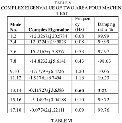
variables. The synchronous machine, the TCSC and the e xciter are described respectively by 6, 3 and 2 state variables. The eigenstructure of the state matrix contains 3 pairs of co mp le x e igenvalues and 5 rea l e igenvalues which are detailed in tables I and I1 respectively.

Eigenvalues accurately determine linear systems stability: this system is close to instability due to the presence of a poorly damped oscillatory mode. Ho wever, if the connections between eigenvalues and state variables are sought, participation factors have to be used. Table III details the participation of the generator subsystems: rotor dynamics, synchronous machine, e xc iter, and TCSC in a ll modes. Table III c learly indicates that the poorly damped oscillatory mode (eigenvalues 1 and 2) is associated to the rotor dynamics and that the other oscillatory mode (eigenvalues 3 and 4) describes the interaction between the synchronous mach ine and the e xcite r. The mode associated to the rotor dynamics is a lso known as electro mechanica l mode. Table III also shows that three e xponential modes are associated to the machine (da mper windings), other two to TCSC and the remaining mode to the exciter. The slower

modes correspond to the TCSC dynamics whereas the fastest mode is associated to the exciter

sTw sTw



1

m

sT 

1 1

lead lag

sT sT

 

1 1

P

K

lead lag

sT sT

 

1 1 Kp

Fig.4 POD Controller structure

1

t

E

P Q

B

E j0.15

j0.93

2200MVA

2

Fig.5 SMIB with TCSC device

TCSC 3

4

B

Power system stabilizer

Design of power system stabilizers or power oscillat ion

damper (POD) in case of FA CT can also be addressed using eigenvalue methods. Eigenvalue sensitivities with respect to the parameters of the stabilizer provide a first order approximation o f the e igenvalue movement in the co mp le x plane when those parameters are varied. Prec isely, the residue of the transfer function between the stabilizers

output (reference o f the e xcitation system, ΔVr) and the

stabilizer input (speed, Δ w, termina l voltage, ΔVt , e lectric

power, ΔPg) indicates the magnitude and direction of the

eigenvalue movement in the co mple x p lane when a static

controller is considered able. Table IVcontains the residues

of transfer functions relevant in stabilizer design corresponding to the electromechanica l mode. The phase of the residue informs about the phase compensation required at the eigenvalue frequency so the phase of the eigenvalue

sensitivity becomes 1800 and the magnitude ofthe residue

determines the gain required to achieve the desired

damping. A speed stabilize r requires almost 900 of phase

compensation whereas accelerating power or electric powe r stabilizers do not require phase compensation. The gain of the speed stabilize r will be greater than the gains of either accelerating or electric power stabilizers.

C Analysis of two areas four machine with TCSC

In this study, a two area interconnected four machine power

system shown in Fig.6is considered. The system consists of

four mach ines arranged in two areas inter-connected by a weak tie line [14].

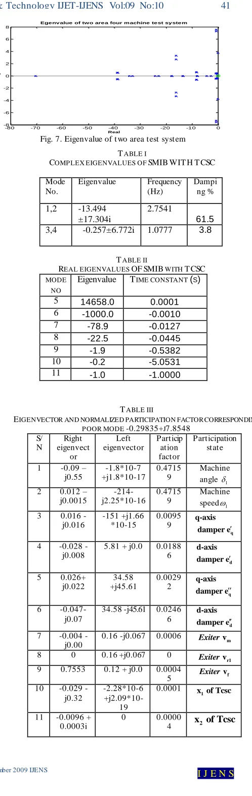
Fig. 7 contains a plot of the eigenvalues in the comp le x plane. Three pairs of poorly da mped eigenvalues are found. They result to be associated to the rotor dynamics. The slowest eigenvalues are associated to the speed -governing systems whereas the fastest are associated to the excitation systems. The synchronous machine modes are in between. Fro m the table V, we see that the system is stable. There are four rotor angle modes. There mode shapes are described by the component of the right eigenvector corresponding to the generator speed

V. DESIGNOFTCSCPODCONTROLLERUSING

RESIDUEMETHOD

The uncontrolled system, Fig.6, has one inter-a rea

oscillatory mode characterized by λ = -0.1211 ± j3.7559

with damping ratio ζ= 3.22%. According to Table VII, the

bus 8 has the largest residue and therefore the most effective location of the SVC and to apply the feedback control. Using the method presented in

1

2

3

4 7

8 5

1 6 9 10 11

L7 L9

Fig. 6 Two area test system with TCSC

G1

G2

G3

G4

-80 -70 -60 -50 -40 -30 -20 -10 0

-8 -6 -4 -2 0 2 4 6 8

Real

Im

ag

Egenvalue of two area four machine test system

Fig. 7. Eigenvalue of t wo area test system TABLEI

COMP LEX EIGENVALUES OF SMIBWIT HT CSC

Mode No.

Eigenvalue Frequency (Hz)

Dampi ng %

1,2 -13.494 ±17.304i

2.7541

61.5

3,4 -0.257±6.772i 1.0777 3.8

TABLEII

REAL EIGENVALUES OFSMIB WITH T CSC

MODE

NO

Eigenvalue TIME CONSTANT (S)

5 14658.0 0.0001

6 -1000.0 -0.0010

7 -78.9 -0.0127

8 -22.5 -0.0445

9 -1.9 -0.5382

10 -0.2 -5.0531

11 _{-1.0 -1.0000}

TABLEIII

EIGENVECTOR AND NORMALIZED PARTICIPATION FACTOR CORRESPONDING

P OOR MODE -0.29835+J7.8548

S/ N

Right eigenvect

or

Left eigenvector

Particip ation factor

Participation state

1 -0.09 – j0.55

-1.8*10-7 +j1.8*10-17

0.4715 9

Machine angle 1 2 0.012 –

j0.0015

-214-j2.25*10-16

0.4715 9

Machine speed1 3 0.016 -

j0.016

-151 +j1.66 *10-15

0.0095

9 _

q

q-axis damper e

4 -0.028 - j0.008

5.81 + j0.0 0.0188

6 _

d

d-axis damper e

5 0.026+ j0.022

34.58 +j45.61

0.0029

2 _

q

q-axis damper e

6 -0.047- j0.07

34.58 -j45.61 0.0246

6 _

d

d-axis

damper e

7 -0.004 - j0.00

0.16 -j0.067 0.0006 Exiter vm

8 0 0.16 +j0.067 0 _Exiter

r1

v

9 0.7553 0.12 + j0.0 0.0004

5 Exiter vf 10 -0.029 -

j0.32

-2.28*10-6

+j2.09*10-19

0.0001

1

x of Tcsc

11 -0.0096 + 0.0003i

0 0.0000

International Journal of Engineering & Technology IJET-IJENS Vol:09 No:10 42

Section 3, POD controller para meters are calcu lated in o rder to shift the real part of the oscillatory mode, to the left half comple x p lane. The obtained transfer function for the SVC POD controller is

1 10 1 0 1329 1 0 1329

1 0 1 1 10 1 0 4325 1 0 4325

s s s

H s K

s s s s

 



   

. .

( ) * * *

. . .

Eigenvalue of our interest moves form the original location

λ = -0.1211 ± j3.7559 to the desired location λd= -0.745 ±

j3.638 to give about 20% damping as:

1

25 8963.

( )

i d

i i

K R H

   

 

VI. SIMULAT ION RESULTS

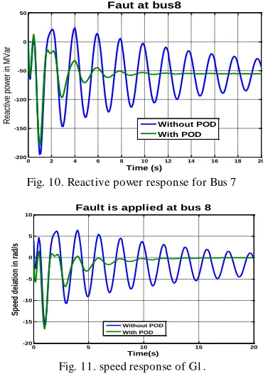
The effectiveness of the proposed method of POD designed was tested on two- area four -machine systems. The analysis results for the two systems are presented in tables I to IX. A three phase fault is applied for second test model at the bus 8 and cleared after 74ms. The origina l system is restored

upon the fault clearance. The transient stability

performances of the system with TCSC without POD and TCSC with POD controller are shown in fig.s 8-11. The TCSC with damping controlle r stabilizes system as can be

seen from fig. 8-11.The oscillations of the system fro m fig.

8 to 11 also are well damped with POD controller.

ACKNOWLEDGMENT

The authors would like to e xpress their appreciation to the Universiti Te knologi Malaysia (UTM) and Min istry of Science Technology and Innovation (MOSTI) for funding this research

CONCLUSION

This paper has reviewed methods for analysis and control of power system oscillations with TCSC device based on the eigenstructure of the state matrix of the linear model of the power system. Residue-based methods also provide valuable informat ion on how to design power system damping controllers. Although eigenvalue based methods are very powerful, the co mple xity of the power system stability problem requires the comple mentary use of other methods such as non-linear time do ma in simulation. A ll the simu lations were done with PST toolbo x in Matlab environment.

APPENDIX

TCSC data

Tr = 10 ms, XL = 0.2, XC=0.1,.Kc=50% Kr=10, TW = 10 s, αMAX =3.1416, αMIN =- 0.314

TABLEIV

RESIDUE CORRESPONDING TO LOCAL MODE -0.257-J6.772

T ransfer function Residue Phase angle

g

r P

V

 

-56.15- 133.27 67.150

r

V







-0.1252 + 0.0585i -25.044

1

r

V V 



0.0429 - 0.0087i -11.46

0 5 10 15 20 25

-150 -100 -50 0 50 100 150 200 250 300

Time(s)

Act

ive

po

we

r in

MW

Fault at bus 8

without POD controller with POD controller

Fig. 8. Active power flow with and without POD in line 7 -8

0 2 4 6 8 10 12 14 16 18 20

-60 -50 -40 -30 -20 -10 0 10 20

Tim e (s)

Angle deviaton

(G1-G3)

Fault at bu 8

without POD with POD

Fig. 9. Angle response of G1 TABLEV

COMPLEXEIGENVALUEOFT WOAREAFOURMACHINE T EST

Mode

No. C omplex Eigenvalue

Frequen cy (Hz)

Damping ratio % 1,2 -12.3267±j 20.5784 0.08 99.99 3,4 -12.0224 ±j19.9823 0.08 99.99

5,6 -15.2167±j15.8377 0.53 97.97

7,8 -14.8232 ±j 5.6141 0.43 -98.63

9,10 -1.7779 ±j 6.4726 1.20 10.05 11,12 -1.9176±j 6.7494 1.16 10.23

13,14 -0.11727±j 3.6383 0.60 3.22

15,16 -5.1493±j 0.04188 0.10 99.72

17,18 -0.07742±j .22111 0.09 99.76

T ABLEVI

PARTICIP ATION OF THE GENERATORS IN THE ELECTROMECHNICAL

MODES OF THE TWO AREA TEST SYSTEM

Mode No.

Eigenvalue G1 G2 G3 G4

9,10 0.7647 ±7.5680i

0.011 45

0.042 9

0.41 007

0.55 216

11,12

0.7514 ±7.3036i

0.411 04

0.536 42

0.02 767

0.01 232

13,14

0.1211 ±3.7559i

0.246 13

0.141 99

0.34 591

0.24 344

TABLE VII

SIT INGINDICESOF TCSC FOR TWO AREA FOUR MACHINE TEST

Mode residues of the transfer function ΔP/Δkc

TCSC location

0 2 4 6 8 10 12 14 16 18 20 -200

-150 -100 -50 0 50

Time (s)

R

ea

ct

ive

p

ow

er

in

MVa

r

Faut at bus8

Without POD With POD

Fig. 10. Reactive power response for Bus 7

0 5 10 15 20 -20

-15 -10 -5 0 5 10

Time(s)

Sp

ee

d

d

ei

ati

o

n

in

r

ad

/s

Fault is applied at bus 8

Without POD With POD

Fig. 11. speed response of G1.

REFERENCES

[1] B. Kalyan Kumar, S.N. Singh and S.C. Srivastava ‖Placement of SVC controllers using modal controllability indices to damp out power system oscillations‖ IET Gener. Transmission . Distrib., Vol. 1, No. 2, page 209-217, March 2007

[2] RJ. Piwko, Ed., ‗‘Applications of Static Var System s for System Dynam ic Performance’’ IEEE Publication 87TH01875-5-PWR, [3] N.G. Hingorani, ― Flexible ac transmission‖, lEEE Spectrum , April

1993, pp. 40-45.

[4] M. A. Pai and Alex Stankovic Robust control in power system tex book. USA, Springer Science+Business Media, Inc. 2005

[5] S.N. Singh, A.K. David ―A New Approach for Placement of FACT S Devices in Open Power Markets‖ IEEE Power Engineering Review, September 2001pp 58-60

[6] K.R. Padiyar ―Power system dynamics stability and Control‖ Anshan limited UK 2004

[7] kamoto, H., Kurita, A., and Sekine, Y.: ‗A method for identification of effective locations of variable impedance apparatus on enhancement of steady state stability in large scale power systems‘, IEEE T rans. Power Syst., 1995, 10, (3), pp. 1401–1407

[8] E. Acha, C. Fuerte-Esquivel, H. Ambriz-Perez and C. Angeles- Camacho. FACT S Modelling and Simulation in Power Networks, John Wiley & Sons LTD, England, 2004.

[9] C. A. Cañizares and Z. T . Faur, ―Analysis of SVC and T CSC Controllers in Voltage Collapse ,‖ IEEE Trans. Power System s, Vol. 14, No. 1, February 1999, pp. 158-165.

[10] G. Hingorani and L. Gyugyi, Understanding FACTS: Concepts and Technology of Flexible AC Transmission Systems, IEEE Press, 1999. [11]Federico Milano, Power System Analysis Toolbox Documentation for

PSAT version 2.0.0 β, March 8, 2007

[12] D.Jovcic, G.N.Pillai "Analytical Modelling of T CSC Dynamics" IEEE Transactions on Power Delivery, vol 20, Issue 2, April 2005, pp. 1097-1104

[13] Y.H. Song and A.T. Johns. ‗‘Flexible AC Transmission Systems‘'. IEE Power and energy series, UK, 1999.

[14] Kundur P. Power system stability and control. New York, USA: McGraw- Hill; 1994.

[15] Bikash Pal , Balarko Chaudhuri ― Robust Control in power System‖ Springer Science+Business Media, Inc.USA 2005

[16] J. Perez-Arriaga, G.C. Verghese, F.C. Schweppe, ― Selective Modal Analysis with Applications to Electric Power Systems. Part I:Heuristic Introduction. Pant 11: The Dynamic Stability Problem‖.

IEEE Transactions on Power Apparatus andsystem s, Vol. PAS-101,

No. 9, September 1982, pp. 3117-3134