189 |
P a g e
FACE RECOGNITION USING PRINCIPAL
COMPONENT ANALYSIS (PCA)
K.Yaswanth Krishna
Dept of ECE, Sir C.R. Reddy College of Engineering,
Eluru of Andhra University, Visakhapatnam. (India)
ABSTRACT
It has been observed that different approaches to the face recognition problem fall into two major categories.
Feature based recognition
Principal component analysis
We present an approach to the detection and identification of human faces and describe a working, near real time face recognition system using PRINCIPAL COMPONENT ANALYSIS (PCA). This approach transforms face images into a small set of characteristic feature images called ‘Eigen faces’, which are the principal components of initial training set of face images. so, goal is to find out Eigen vectors(Eigen faces) of the co-variance matrix of the distribution, spanned by a training set of face images.
Recognition is performed by projecting a new image into subspace spanned by Eigen faces and then classifies the face by comparing its position in face space with the positions of known individuals. PCA approach seems to be an adequate method to be used in face recognition due to simplicity, speed and learning capability.
I INTRODUCTION
Much of the previous work on automated face recognition has ignored the issue of just what aspects of the face
stimulus are important for face recognition. This suggests the use of an information theory approach of coding and
decoding of face images, emphasizing the significant local and global features. Such features may or may not be
directly related to our intuitive notion of face features such as the eyes, nose, lips, and hair.
In the language of information theory, the relevant information in a face image is extracted, encoded as efficiently as
possible, and then compared with a database of models encoded similarly. A simple approach to extracting the
information contained in an image of a face is to somehow capture the variation in a collection of face images,
independent of any judgment of features, and use this information to encode and compare individual face images.
In mathematical terms, the principal components of the distribution of faces, or the eigenvectors of the covariance
matrix of the set of face images, treating an image as point (or vector) in a very high dimensional space is sought.
The eigenvectors are ordered, each one accounting for a different amount of the variation among the face images.
These eigenvectors can be thought of as a set of features that together characterize the variation between face
images.
Each image location contributes more or less to each eigenvector, so that it is possible to display these eigenvectors
190 |
P a g e
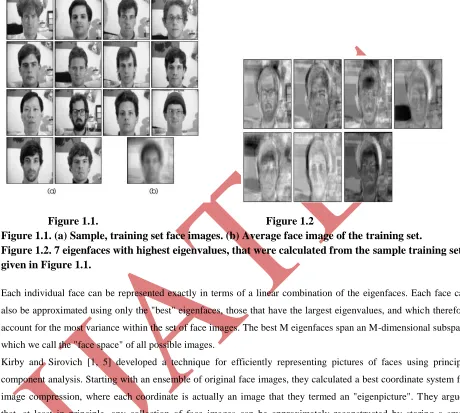
Sample face images and the corresponding eigenfaces are shown in Figure 1.1-a and in Figure 1.2 respectively. Each
eigenface deviates from uniform gray where some facial feature differs among the set of training faces. Eigenfaces
can be viewed as a sort of map of the variations between faces.
Figure 1.1. Figure 1.2
Figure 1.1. (a) Sample, training set face images. (b) Average face image of the training set.
Figure 1.2. 7 eigenfaces with highest eigenvalues, that were calculated from the sample training set,
given in Figure 1.1.
Each individual face can be represented exactly in terms of a linear combination of the eigenfaces. Each face can
also be approximated using only the "best" eigenfaces, those that have the largest eigenvalues, and which therefore
account for the most variance within the set of face images. The best M eigenfaces span an M-dimensional subspace
which we call the "face space" of all possible images.
Kirby and Sirovich [1, 5] developed a technique for efficiently representing pictures of faces using principal
component analysis. Starting with an ensemble of original face images, they calculated a best coordinate system for
image compression, where each coordinate is actually an image that they termed an "eigenpicture". They argued
that, at least in principle, any collection of face images can be approximately reconstructed by storing a small
collection of weights for each face, and a small set of standard pictures (the eigenpictures). The weights describing
each face are found by projecting the face image onto each eigenpicture.
In this thesis, we have followed the method which was proposed by M. Turk and A. Pentland [11] inorder to develop
a face recognition system based on the eigenfaces approach. They argued that, if a multitude of face images can be
reconstructed by weighted sum of a small collection of characteristic features or eigenpictures, perhaps an efficient
way to learn and recognize faces would be to build up the characteristic features by experience over time and
recognize particular faces by comparing the feature weights needed to approximately reconstruct them with the
191 |
P a g e
eigenpicture weights needed to
describe and reconstruct them. This is an extremely compact representation
when compared with the images themselves.
II FACE RECOGNITION SYSTEM
The proposed face recognition system passes through three main phases during a face recognition process. Three
major functional units are involved in these phases and they are depicted in Figure 1.3. The characteristics of these
phases in conjunction with the three functional units are given below:
2.1 Face Library Formation Phase
In this phase, the acquisition and the preprocessing of the face images that are going to be added to the face library
are performed. Face images are stored in a face library in the system. We call this face database a "face library"
because at the moment, it does not have the properties of a relational database. Every action such as training set or
eigenface formation is performed on this face library. Face library is initially empty. Inorder to start the face
recognition process, this initially empty face library has to be filled with face images.
The proposed face recognition system operates on 128 x 128 x 8, HIPS formatted image files. At the moment,
scanner or camera support is unavailable. Inorder to perform image size conversions and enhancements on face
images, there exists the "pre-processing" module. This module automatically converts every face image to 128 x 128
(if necessary) and based on user request, it can modify the dynamic range of face images (histogram equalization) in
order to improve face recognition performance. Also, we have considered implementing a "background removal"
algorithm in the pre-processing module, but due to time limitations, we have left this for future work.
After acquisition and pre-processing, face image under consideration is added to the face library. Each face is
represented by two entries in the face library. One entry corresponds to the face image itself (for the sake of speed,
no data compression is performed on the face image that is stored in the face library) and the other
corresponds to the weight vector associated for that face image. Weight vectors of the face library members are
empty until a training set is chosen and eigenfaces are formed.
2.2 Training Phase
After adding face images to the initially empty face library, the system is ready to perform training set and eigenface
formations. Those face images that are going to be in the training set are chosen from the entire face library.
Because that the face library entries are normalized, no further pre-processing is necessary at this step. After
choosing the training set, eigenfaces are formed and stored for later use.
Eigenfaces are calculated from the training set, keeping only the M images that correspond to the highest
eigenvalues. These M eigenfaces define the M-dimensional "face space". As new faces are experienced, the
eigenfaces can be updated or recalculated. The corresponding distribution in the M-dimensional weight space is
calculated for each face library member, by projecting its face image onto the "face space" spanned by the
192 |
P a g e
Now the corresponding weight vector of each face library member has been updated which were initially empty.
The system is now ready for the recognition process. Once a training set has been chosen, it is not possible to add
new members to the face library with the conventional method that is presented in "phase
1" because, the system
does not know whether this item already exists in the face library or not. A library search must be
performed.
2.3 Recognition and Learning Phase
After choosing a training set and constructing the weight vectors of face library members, now the system is ready
to perform the recognition process. User initiates the recognition process by choosing a face image. Based on the
user request and the acquired image size, pre-processing steps are applied to normalize this acquired image to face
library specifications (if necessary).
After obtaining the weight vector, it is compared with the weight vector of every face library member within a user
defined "threshold". If there exists at least one face library member that is similar to the acquired image within that
threshold then, the face image is classified as "known".
Otherwise, a miss has occurred and the face image is classified as "unknown". After being classified as unknown,
this new face image can be added to the face library with its corresponding weight vector for later use (learning to
recognize).
193 |
P a g e
III EIGEN FACE BASED FACIAL RECOGNITION SYSTEM
IV CALCULATING EIGEN FACES
Let a face image I(x,y) be a two-dimensional N x N array of 8-bit intensity values. An image may also be considered
as a vector of dimension N2 , so that a typical image of size 256 x 256 becomes a vector of dimension 65,536, or
equivalently a point in 65,536-dimensional space. An ensemble of images, then, maps to a collection of points in
this huge space.
Images of faces, being similar in overall configuration, will not be randomly distributed in this huge image space
and thus can be described by a relatively low dimensional subspace. The main idea of the principal component
analysis (or Karhunen-Loeve expansion) is to find the vectors that best account for the distribution of face images
within the entire image space.
These vectors define the subspace of face images, which we call "face space". Each vector is of length N2 ,
194 |
P a g e
eigenvectors of the covariance matrix corresponding to the original face images, and because they
are face-like in
appearance, we refer to them as "eigenfaces". Some examples of eigenfaces are shown in Figure 1.2.
DEFINITIONS
An N x N matrix A is said to have an eigenvector X, and corresponding eigenvalue l if
AX = X. (1.1)
Evidently, Eq. (1.1) can hold only if
det {A- I}=0. (1.2)
Which, if expanded out, is an Nth degree polynomial in whose root are the eigenvalues. This proves that there are always N (not necessarily distinct) eigenvalues. Equal eigenvalues coming from multiple roots are called "degenerate".
A matrix is called symmetric if it is equal to its transpose, A= ATor aij= aji (1.3)
It is termed orthogonal if its transpose equals its inverse,
AT A= AAT = I (1.4)
finally, a real matrix is called normal if it commutes with is transpose,
A AT = AT A. (1.5)
THEOREM
Eigen values of a real symmetric matrix are all real. Contrariwise, the Eigen values of a real non-symmetric matrix
may include real values, but may also include pairs of complex conjugate values. The Eigen values of a normal
matrix with non-degenerate Eigen values are complete and orthogonal, spanning the N-dimensional vector space.
After giving some insight on the terms that are going to be used in the evaluation of the Eigen faces, we can deal
with the actual process of finding these eigen faces.
Let the training set of face images be then the average of the set is defined by
(1.6)
Each face differs from the average by the vector
(1.7)
An example training set is shown in Figure 1.1-a, with the average face Y shown in Figure 1.1-b. This set of very
large vectors is then subject to principal component analysis, which seeks a set of M orthonormal vectors, un , which
best describes the distribution of the data. The kth vector, uk , is chosen such that
(1.8)
is a maximum, subject to
195 |
P a g e
The vectors uk and scalars are the eigenvectors and eigen values, respectively of the covariance matrix
(1.10)
where the matrix
The covariance matrix C, however is N2xN2 real symmetric matrix, and determining the N2 eigenvectors and
eigenvalues is an intractable task for typical image sizes. We need a computationally feasible method to find these
eigenvectors.
If the number of data points in the image space is less than the dimension of the space (M < N2 ), there will be only
M-1, rather than N2 , meaningful eigenvectors. The remaining eigenvectors will have associated eigenvalues of zero.
We can solve for the N2 dimensional eigenvectors in this case by first solving the eigenvectors of an M x M matrix
such as solving 16 x 16 matrix rather than a 16,381 x 16,381 matrix and then, taking appropriate linear combinations
of the face images i.
Consider the eigenvectors Viof A
T
Asuch that
ATAVi = µiVi (1.11)
Pre-multiplying both sides by A, we have
AAT AVi = µi AVi (1.12)
from which we see that AVi are the eigenvectors of C= AAT .
Following these analysis, we construct the M x M matrix L = AT A, where
and find the M eigenvectors, vi, of L. These vectors determine linear combinations of the M training set face images
to form the eigenfaces ui.
(1.13)
With this analysis, the calculations are greatly reduced, from the order of the number of pixels in the images (N2 ) to
the order of the number of images in the training set (M). In practice, the training set of face images will be
relatively small (M << N2 ), and the calculations become quite manageable. The associated eigenvalues allow us to
rank the eigenvectors according to their usefulness in characterizing the variation among the images.
V USING EIGEN FACES TO CLASSIFY A FACE IMAGE
The eigen face images calculated from the eigenvectors of L, span a basis set with which to describe face images.
196 |
P a g e
males digitized in a controlled manner, and found that 10 eigenfaces were sufficient for a very good description of
face images. With M' = 10 eigenfaces, RMS pixel by pixel errors in representing cropped versions of face images
were about 2%.
In practice, a smaller M' can be sufficient for identification, since accurate reconstruction of the image is not a
requirement. Based on this idea, the proposed facerecognition system lets the user specify the number of eigenfaces
(M') that is going to be used in the recognition. For maximum accuracy, the number of eigenfaces should be equal to
the number of images in the training set. But, it was observed that, for a training set of fourteen face images, seven
eigenfaces were enough for a sufficient description of the training set members. In this framework, identification
becomes a pattern recognition task. The eigenfaces span an M' dimensional subspace of the original N2 image space.
The M' significant eigenvectors of the L matrix are chosen as those with the largest associated eigenvalues. A new
face image (G ) is transformed into its eigenface components (projected onto "face space") by a simple operation,
(1.11)
for k = 1,...,M'. This describes a set of point by point image multiplications and summations, operations performed
at approximately frame rate on current image processing hardware, with a computational complexity of O(N1 ).
The weights form a feature vector,
(1.15)
that describes the contribution of each eigenface in representing the input face image, treating the eigenfaces as a
basis set for face images. The feature vector is then used in a standard pattern recognition algorithm to find which of
a number of predefined face classes, if any, best describes the face. The face classes Wi can be calculated by
averaging the results of the eigenface representation over a small number of face images (as few as one) of each
individual. In the proposed face recognition system, face classes contain only one representation of each individual.
Classification is performed by comparing the feature vectors of the face library members with the feature vector of
the input face image. This comparison is based on the Euclidean distance between the two members to be smaller
than a user defined threshold e k . This is given in Eq. (1.16). If the comparison falls within the user defined
threshold, then face image is classified as “known”, otherwise it is classified as “unknown” and can be added to face
library with its feature vector for later use, thus making the system learning to recognize new face images.
197 |
P a g e
VI RE-BUILDING A FACE IMAGE WITH EIGEN FACES
A face image can be approximately reconstructed (rebuilt) by using its feature vector and the eigenfaces as
(1.17) Where
(1.18)
is the projected image.Eq. (1.17) tells that the face image under consideration is rebuilt just by adding each
eigenface with a contribution of wiEq. (1.18) to the average of the training set images. The degree of the fit or the
"rebuild error ratio" can be expressed by means of the Euclidean distance between the original and the reconstructed
face image as given in Eq. (1.19). It has been observed that, rebuild error ratio increases as the training set members
differ heavily from each other. This is due to the addition of the average face image. When the members differ from
each other (especially in image background) the average face image becomes more messy and this increases the
rebuild error ratio.
(1.19)
There are four possibilities for an input image and its pattern vector:
1. Near face space and near a face class,
2. Near face space but not near a known face class,
3. Distant from face space and near a face class,
1. Distant from face space and not near a known face class.
In the first case, an individual is recognized and identified. In the second case, an unknown individual is presented.
The last two cases indicate that the image is not a face image.
Case three typically shows up as a false classification. It is possible to avoid this false classification in this system by
using Eq. (1.18) as
(1.20)
where kis a user defined threshold for the faceness of the input face images belonging to kth face class.
VII SUMMARY OF EIGEN FACE RECOGNITION PROCEDURE
The eigenfaces approach to face recognition can be summarized in the following steps:
198 |
P a g e
Choose a training set that includes a number of images (M) for each person with some variation in expression
and in the lighting.
Calculate the M x M matrix L, find its eigenvectors and eigenvalues, and choose the M' eigenvectors with the
highest associated eigenvalues.
Combine the normalized training set of images according to Eq. (1.13) to produce M' eigenfaces. Store these eigenfaces for later use.
For each member in the face library, compute and store a feature vector according to Eq. (1.15).
Choose a threshold e according to (1.16) that defines the maximum allowable distance from any face class.
Optionally choose a threshold f according to Eq. (1.20) that defines the maximum allowable distance from
face space.
For each new face image to be identified, calculate its feature vector according to Eq. (1.15) and compare it with
the stored feature vectors of the face library members. If the comparison satisfies the condition given in Eq.(1.16)
for at least one member, then classify this face image as "known", otherwise a miss has occurred and classify it
as "unknown" and add this member to the face library with its feature vector.
VIII ACKNOWLEDGEMENTS
I would like to thank the faculty members in Department of ECE, Andhra University, Visakhapatnam and the
management and higher officials of SIR C R Reddy college of Engineering for extending their cooperation in
continuing the research.
IX CONCLUSIONS
Early attempts at making computers recognize faces were limited by the use of impoverished face models and
feature descriptions (locating features from an edge image and matching simple distances and ratios ), assuming that
a face is no more than the sum of its parts, the individual features.
Recent attempts using parameterized feature models and multi-scale matching look more promising, but still face
severe problems before they are generally applicable. Current connectionist approach tend to hide much of the
pertinent information in the weights that makes it difficult to modify and evaluate parts of the approach.
The eigen face approach to face recognition was motivated by information theory, leading to the idea of basing face
recognition on a small set of features that best approximate the set of known face images, without requiring that they
correspond to our intuitive notions of facial parts and features.
Although, it is not an elegant solution to the general recognition problem, the eigen face approach does provide a
practical solution to the general recognition problem, the eigen face approach thus provide a practical solution that is
well fitted to the problem of face recognition. It is fast, relatively simple, and has been shown work to well in a
constrained environment. It also can be implemented in a constrained environment. It can also be implemented using
199 |
P a g e
It is important to note that many applications of face recognition do not require perfect identification, although most
require a low false-positive rate. In searching a large database of faces, for example, it may be preferable to find a
small set of likely matches to present to the user.
For applications such as security systems or human computer interaction, the system will normally be able to view
the subject for a few seconds or minutes, and thus will have number of chances to recognize the person. Experiments
show that the eigen face technique can be made to perform at very high accuracy, although with a substantial
unknown rejection, and thus is potentially well suited to these applications.
BIBILIOGRAPHY
1. DIGITAL IMAGE PROCESSING
Rafael C. Gonzalez
Richard E. Woods
2. PATTERN RECOGNITION AND IMAGE ANALYSIS
Earl Gose
Richard Jhonson Baugh
3. MASTERING MATLAB 7
Duane Hanselman
Bruce Little field
4. DIGITAL IMAGE PROCESSING USING MATLAB
Rafael C. Gonzalez
Richard E. Woods
5. FACE RECOGNITION USING EIGEN FACES
Mattew A.Turk
Alex P.Pentland
K.YaswanthKrishna is pursuing the bachelor’s degree in electronics communication engineering from SIR C.R.Reddy College of Engineering, Eluru of Andhra University,