ISSN 2307-7743 http://scienceasia.asia
A GENERALIZED POWER LINDLEY DISTRIBUTION WITH APPLICATIONS
GAYAN WARAHENA-LIYANAGE AND MAVIS PARARAI
Abstract. The Exponentiated Power Lindley (EPL) distribution which is an extension
of the Power Lindley Distribution is introduced and its properties are explored. This new distribution represents a more flexible model for the lifetime data. Some statistical properties of the proposed distribution including the shapes of the density and hazard rate functions, the moments and moment generating function, skewness and kurtosis are explored. Entropy measures and the distribution of the order statistics are given. The maximum likelihood estimation technique is used to estimate the model parameters and finally an application of the model with a real data set is presented for the illustration of the usefulness of the proposed distribution.
1. Introduction
The power Lindley (PL) distribution was proposed by Ghitany et al. [4]. This distribu-tion is an extension of the Lindley (L) distribudistribu-tion which was proposed by Lindley [7] in the context of fiducial and Bayesian statistics. Properties and applications of the Lindley distribution have been studied in the context of reliability analysis by Ghitany et al. [3]. Several other authors including Sankaran [13], Asgharzadeh et al. [1] and Nadarajah et al. [8] proposed and developed the mathematical properties of the generalized Lindley distribution. The probability density function (pdf) of the Lindley distribution is given by,
(1.1) f(y;β) = β
2
β+ 1(1 +y)e
−βy, y >0, β >0.
Using the transformation X = Y 1α, Ghittany et al. [4] derived the power Lindley (PL)
distribution given by
(1.2) f(x;α, β) = αβ
2
β+ 1(1 +x α
)xα−1e−βxα, x >0, α >0, β >0.
The survival function and cumulative distribution function (cdf) of the power Lindley dis-tribution are
S(x) =
1 + βx α
β+ 1
e−βxα,
(1.3)
2010Mathematics Subject Classification. 62F10, 62F12.
Key words and phrases. Exponentiated power Lindley distribution, Power Lindley distribution, Maximum likelihood estimation.
c
2014 Science Asia
and
F(x) = 1−S(x) = 1−
1 + βx α
β+ 1
e−βxα,
(1.4)
for x >0, α, β >0,respectively.
The purpose of this paper is to develop a three-parameter alternative to several lifetime distributions including the gamma, Weibull, exponentiated Weibull, exponentiated Lindley, and lognormal distributions. In this context, we propose and develop the statistical proper-ties of the exponentiated power Lindley (EPL) distribution and show that it is a far better model for reliability analysis.
Our aim in this paper is to discuss some important statistical properties of the EPL distribution. This discussion includes the shapes of the density function and hazard rate function, reversed hazard rate function, moments, moment generating function, distribution of order statistics and model parameter estimation by using the maximum likelihood method. Finally, applications of the model to real data sets in order to illustrate the applicability and usefulness of the EPL distribution are presented.
This paper is organized as follows: In section 2, the model and some of its statistical properties including shapes and behavior of the hazard function are presented. Distribution of order statistics, Moments and related measures are given in section 3. Section 4 contains entropy measures. In section 5,mean deviations, Lorenz and Bonferroni curves are presented. In section 6, we present the maximum likelihood method for estimating the parameters of the distribution. Applications are given in section 7 and thereafter the concluding remarks.
2. The Model, Sub-models and Properties
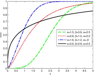
In this section, the cdf, pdf, hazard and reverse hazard functions, and their shapes are presented. We will define G(x) = [F(x)]ω for ω > 0 where F(x) is the cdf of the power Lindley distribution given in (1.4).
G(x;α, β, ω) =
1−
1 + βx α
β+ 1
e−βxα
ω
, x >0, α >0, β >0, ω >0.
(2.1)
Figure 2.1. Plot of the CDF for different values of α, β and ω
The pdf of the EPL distribution is given by
g(x;α, β, ω) = αβ
2ω
β+ 1(1 +x α)xα−1
e−βxα
1−
1 + βx α
β+ 1
e−βxα
ω−1
,
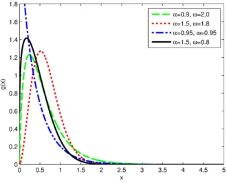
for x > 0, α > 0, β > 0, ω > 0. Plots for the pdf of EPL distribution are given below and each plot has been generated by fixing one parameter at a time.
• α is fixed: see figure 2.1.
• β is fixed: see figure 2.2.
Figure 2.2. Plot of the PDF for different values ofβ, ω and α = 1.5
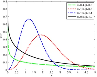
Figure 2.4. Plot of the PDF for different values ofα, β and ω = 1.8
The pdf of the EPL distribution is unimodal. It increases and decreases for various values of the parameters giving the shapes obtained in the above plots. The plots in figs 2.3 and 2.4 show that for α < 1, the pdf is decreasing and for values of α >1, the pdf is unimodal. For values of ω >1, β >1, the graph seems almost symmmetric.
2.1. Sub-models. Some sub-models of the EPL distribution are presented in this section.
• When ω= 1, we obtain the PL distribution.
• When α= 1,we obtain the exponentiated Lindley (EL) distribution.
• When ω=α= 1,we obtain the Lindley (L) distribution.
• When β = 1, we obtain exponentiated two-component mixture of Weibull distribu-tion (with shape parameter α and scale 1) and a gamma distribution (with shape parameter 2α and scale 1).
• Whenα = 2,we obtain an exponentiated two-component mixture of Rayleigh distri-bution (with scaleβ and scale 2) and a gamma distribution (with shape 4 and scale
β).
2.2. Shapes and Stochastic Orders. In this section, we present the mode and discuss the shape, as well as stochastic orders of the EPL distribution. To obtain the mode, we solve the equation dln(dxg(x)) = 0,for x. Note that
log(g(x)) = log(α) + 2 log(β) + log(ω)−log(1 +β) + log(1 +xα)−βxα
+ (α−1) log(x) + (ω−1) log
1−
1 + βx α
β+ 1
e−βxα
.
so that dln(dxg(x)) = 0, results in
αxα−1
1 +xα −αβx α−1
+α−1
x + (ω−1)
αβ2(1 +xα)xα−1e−βxα (1 +β)−[1 +β(1 +xα)]e−βxα
= 0.
Note that limx→0g(x) =∞, and limx→∞g(x) = 0.
LetXi be distributed according toEP L(α, β, ω),with cdf and pdfGi and gi,respectively for i= 1,2. We say X2 is stochastically greater than X1 in likelihood ratio if g2(x)/g1(x) is
an increasing function of x. It is well known that likelihood ratio order implies failure rate order which in turn implies stochastic order, see Shaked and Shanthikumar [12] for additional details.
• If β1 = β2 and α1 = α2, then X2 is stochastically greater than X1 with respect to likelihood ratio order if and only ifω2 > ω1.
• If α1 = α2 and ω1 = ω2 then X2 is stochastically larger than X1 with respect to
likelihood ratio order if and only ifδ1 > δ2.
Note that
g2(x) g1(x)
= (1 +β1)α2
2ω
2β2(1 +xα2)xα2−α1eβ1x
α1−β
2xα2
(1 +β2)α12ω1β1(1 +xα1)
×
1−
1 + β2x α2 β2+ 1
e−β2xα2
ω2−1
1−
1 + β1x α1 β1+ 1
e−β1xα1
ω1−1.
(2.3)
If β1 =β2, and α1 =α2, then
(2.4) K(x) = ω2
ω1
1−
1 + βx α
1 +β
exp(−βxα)
ω2−ω1 ,
and is such that
K0(x) = ω2(ω2−ω1)
ω1
αβ2
β+ 1(1 +x α
)xα−1exp(−βxα)
×
1−
1 + βx α
β+ 1
e−βxα
ω2−ω1−1
≥0,
(2.5)
if and only if ω2−ω1 ≥0.
2.3. Quantile Function. The quantile function is the solution of the equation
1−
1 +β+βxα β+ 1
e−βxα
ω
=p where 0< p < 1.
Thus, the quantile function, say Q(p), defined by G(Q(p)) =p is the root of the equation,
1−
1 +β+βQ(p)α
β+ 1
exp(−βQ(p)α)
ω
LetZ(p) = −1−β−βQ(p)α. We have
1 +
Z(p)
β+ 1
exp{Z(p) + 1 +β}
ω
= p
1 +
Z(p)
β+ 1
exp{Z(p) + 1 +β} = p1/ω
Z(p) exp{Z(p)} = −(β+ 1)(1−p
1/ω
exp(1 +β) .
So the solution for Z(p) is
Z(p) =W −(β+ 1)(1−p1/ω) exp(−1−β).
for 0< p <1, where W(.) is the Lambert W function, [2]. Now,
−1−β−βQ(p)α = W −(β+ 1)(1−p1/ω) exp(−1−β)
βQ(p)α = −1−β−W −(β+ 1)(1−p1/ω) exp(−1−β).
So we have
Q(p) =
−1− 1 β −
1
βW −(β+ 1)(1−p
1/ω) exp(−1−β) 1/α
.
(2.6)
2.4. Hazard and Reverse Hazard Functions. The survival function for the EPL distri-bution is given by,
G(x;α, β, ω) = 1−G(x;α, β, ω)
= 1−
1−
1 + βx α
β+ 1
e−βxα
ω
.
(2.7)
The hazard and reverse hazard functions are given by
λG(x;α, β, ω) =
g(x;α, β, ω)
G(x;α, β, ω)
= αβ2ω
β+1(1 +x
α)xα−1e−βxαh
1−1 + ββx+1αe−βxαiω−1
1−
1−
1 + βx α
β+ 1
e−βxα
ω ,
and
τG(x;α, β, ω) =
g(x;α, β, ω)
G(x;α, β, ω)
= αβ2ω
β+1(1 +x
α)xα−1e−βxαh
1−1 + βxβ+1αe−βxαiω−1
1−
1 + βx α
β+ 1
e−βxα
ω ,
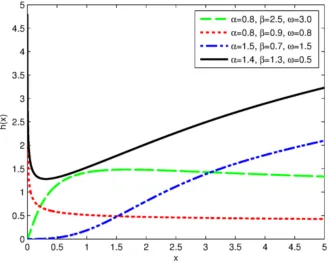
Figure 2.5. Plot of the hazard function for different values of α, β and ω
The graphs of the hazard function for four combinations of the values of the model pa-rameters show various shapes including monotonically increasing, monotonically decreasing, uni-modal, bathtub, and upside down bathtub shapes with four combinations of the values of the parameters. This attractive flexibility makes the EPL hazard rate function useful and suitable for non-monotone empirical hazard behaviors which are more likely to be encoun-tered or observed in real life situations.
3. Moments, Moment Generating Function and Related Measures
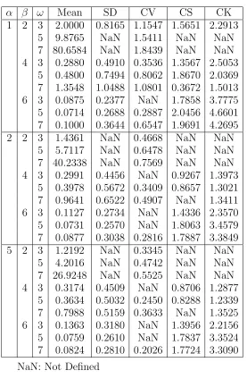
In this section, moments and related measures including coefficients of variation, skewness and kurtosis are presented. A table of values for mean,standard deviation, coefficient of variation (CV), coefficient of skewness (CS) and coefficient of kurtosis (CK) is also presented.
3.1. Moments. The rth moment about the origin of a continuous random variable X, de-noted by µ0r, is ,
µ0r =E(Xr) =
Z ∞
−∞
xrg(x)dx for r = 0,1,2, . . . .
In order to find the moments, consider the following lemma.
Lemma 1
Let,
L1(α, β, ω, r) =
Z ∞
0
xr(1 +xα)xα−1
1−
1 + βx α
β+ 1
e−βxα
ω−1
e−βxαdx
=
Z ∞
0
(1 +xα)xα+r−1
1−
1 + βx α
β+ 1
e−βxα
ω−1
then,
L1(α, β, ω, r) =
∞ X i=0 i X j=0 j+1 X k=0
ω−1
i
i j
j+ 1
k
(−1)iβjΓ(k+rα−1+ 1)
α(β+ 1)i[β(i+ 1)](k+rα−1+1).
Proof. Using the series expansion,
(1−z)a−1 =
∞
X
i=0
a−1
i
(−1)izi,
(3.1)
we have
L1(α, β, ω, r) = ∞
X
i=0
ω−1
i
(−1)i
1 +β(1 +xα)
β+ 1
i
e−iβxα
Z ∞
0
(1 +xα)xα+r−1e−βxαdx
=
∞
X
i=0
ω−1
i
(−1)i (β+ 1)i
Z ∞
0
(1 +xα)xα+r−1[1 +β(1 +xα)]ie(−iβxα−βxα)dx
=
∞
X
i=0
ω−1
i
(−1)i (β+ 1)i
i X j=0 i j βj Z ∞ 0
(1 +xα)j+1xα+r−1e(−iβxα−βxα)dx
= ∞ X i=0 i X j=0 j+1 X k=0
ω−1
i
i j
j+ 1
k
(−1)iβj
(β+ 1)i
Z ∞
0
xα+αk+r−1e−(i+1)βxαdx.
Now consider,
Z ∞
0
xα+αk+r−1e−(i+1)βxαdx.
(3.2)
Letu=β(i+ 1)xα, then du
dx =αβ(i+ 1)x
α−1 and x=
u
(β(i+ 1)
1/α
.
The above integral can rewritten by using the complete gamma function Γ(a) =R0∞xa−1e−xdx
as,
Z ∞
0
u
(β(i+ 1)
(αkα+r)
e−u du
αβ(i+ 1) =
Z ∞
0
u(k+rα−1)e−u
α[β(i+ 1)](k+rα−1+1)du
= Γ(k+rα
−1+ 1)
α[β(i+ 1)](k+rα−1+1). Consequently,
L1(α, β, ω, n) = ∞ X i=0 i X j=0 j+1 X k=0
ω−1
i
i j
j+ 1
k
(−1)iβjΓ(k+rα−1+ 1)
α(β+ 1)i[β(i+ 1)](k+rα−1+1).
Now using Lemma 1, the rth moment of the EPL distribution is given by
µ0r =E(Xr) = αβ
2ω
The first four moments of X can be written as,
µ01 = E(X) = αβ
2ω
β+ 1L1(α, β, ω,1).
µ02 = E(X2) = αβ
2ω
β+ 1L1(α, β, ω,2).
µ03 = E(X3) = αβ
2ω
β+ 1L1(α, β, ω,3).
µ04 = E(X4) = αβ
2ω
β+ 1L1(α, β, ω,4).
The mean, variance, coefficient of variation (CV), coefficient of skewness (CS) and coefficient of kurtosis (CK) are given by
µ=µ01 =E(X) = αβ
2ω
β+ 1L1(α, β, ω,1), (3.4)
σ2 =µ02−µ2,
(3.5)
(3.6) CV = σ
µ =
p
µ02 −µ2
µ =
s
µ02 µ2 −1,
(3.7) CS= E[(X−µ)
3]
[E(X−µ)2]3/2 =
µ03 −3µµ02+ 2µ3
(µ02−µ2)3/2 ,
and
(3.8) CK = E[(X−µ)
4]
[E(X−µ)2]2 =
µ04−4µµ03+ 6µ2µ0
2−3µ4
(µ0
2 −µ2)2
,
α β ω Mean SD CV CS CK 1 2 3 2.0000 0.8165 1.1547 1.5651 2.2913
5 9.8765 NaN 1.5411 NaN NaN
7 80.6584 NaN 1.8439 NaN NaN
4 3 0.2880 0.4910 0.3536 1.3567 2.5053 5 0.4800 0.7494 0.8062 1.8670 2.0369 7 1.3548 1.0488 1.0801 0.3672 1.5013 6 3 0.0875 0.2377 NaN 1.7858 3.7775 5 0.0714 0.2688 0.2887 2.0456 4.6601 7 0.1000 0.3644 0.6547 1.9691 4.2695
2 2 3 1.4361 NaN 0.4668 NaN NaN
5 5.7117 NaN 0.6478 NaN NaN
7 40.2338 NaN 0.7569 NaN NaN
4 3 0.2991 0.4456 NaN 0.9267 1.3973 5 0.3978 0.5672 0.3409 0.8657 1.3021 7 0.9641 0.6522 0.4907 NaN 1.3411 6 3 0.1127 0.2734 NaN 1.4336 2.3570 5 0.0731 0.2570 NaN 1.8063 3.4579 7 0.0877 0.3038 0.2816 1.7887 3.3849
5 2 3 1.2192 NaN 0.3345 NaN NaN
5 4.2016 NaN 0.4742 NaN NaN
7 26.9248 NaN 0.5525 NaN NaN
4 3 0.3174 0.4509 NaN 0.8706 1.2877 5 0.3634 0.5032 0.2450 0.8288 1.2339 7 0.7988 0.5159 0.3633 NaN 1.3525 6 3 0.1363 0.3180 NaN 1.3956 2.2156 5 0.0759 0.2610 NaN 1.7837 3.3524 7 0.0824 0.2810 0.2026 1.7724 3.3090
NaN: Not Defined
Table 3.1. Table of Mean, SD, Coefficient of Variation, Skewness and Kurtosis
Lemma 2
Let,
L2(α, β, ω, r, t) =
Z ∞
t
xr(1 +xα)xα−1
1−
1 + βx α
β+ 1
e−βxα
ω−1
e−βxαdx
=
Z ∞
t
(1 +xα)xα+r−1
1−
1 + βx α
β+ 1
e−βxα
ω−1
e−βxαdx.
then,
L2(α, β, ω, r, t) = ∞ X i=0 i X j=0 j+1 X k=0
ω−1
i
i j
j+ 1
k
(−1)iβjΓ(k+rα−1 + 1, β(i+ 1)tα)
α(β+ 1)i[β(i+ 1)](k+rα−1+1) .
Proof. Using the same procedure that was used in Lemma 1, this can be simplified into the following form.
L2(α, β, ω, r, t) = ∞ X i=0 i X j=0 j+1 X k=0
ω−1
i
i j
j+ 1
k
(−1)iβj
(β+ 1)i
Z ∞
t
xα+αk+r−1e−(i+1)βxαdx.
Now consider,
Z ∞
t
xα+αk+r−1e−(i+1)βxαdx.
Letu=β(i+ 1)xα, then du
dx =αβ(i+ 1)x
α−1 and x=
u β(i+ 1)
1/α
.
The above integral can be rewritten by using the complementary incomplete gamma function Γ(a, t) = Rt∞xa−1e−xdx as,
Z ∞
β(i+1)tα
u β(i+ 1)
(αkα+r)
e−u du
αβ(i+ 1) =
Z ∞
β(i+1)tα
u(k+rα−1) e−u
α[β(i+ 1)](k+rα−1+1)du = Γ(k+rα
−1+ 1, β(i+ 1)tα)
α[β(i+ 1)](k+rα−1+1) . Consequently,
L2(α, β, ω, r, t) = ∞ X i=0 i X j=0 j+1 X k=0
ω−1
i
i j
j+ 1
k
(−1)iβjΓ(k+rα−1 + 1, β(i+ 1)tα)
α(β+ 1)i[β(i+ 1)](k+rα−1+1) .
Now using Lemma 2, the rthconditional moment of the EPL distribution is given by
E(Xr|X > x) = αβ
2ω
β+ 1
L2(α, β, ω, r, x)
1−G(x)
= αβ
2ωL
2(α, β, ω, r, x)
β+ 1 ×
1
1 + ββx+1α
e−βxα
= αβ
2ω
β+ 1
L2(α, β, ω, r, x)
The first four conditional moments are given by,
E(X|X > x) = αβ
2ω
β+ 1
L2(α, β, ω,1, x)
(1 +β+βxα)e−βxα.
E(X2|X > x) = αβ
2ω
β+ 1
L2(α, β, ω,2, x)
(1 +β+βxα)e−βxα.
E(X3|X > x) = αβ
2ω
β+ 1
L2(α, β, ω,3, x)
(1 +β+βxα)e−βxα.
E(X4|X > x) = αβ
2ω
β+ 1
L2(α, β, ω,4, x) (1 +β+βxα)e−βxα.
The mean residual lifetime function is given by E(X|X > x)−x.
3.3. Moment Generating Function. The moment generating function (MGF) of a con-tinuous random variable X, where it exists, is given by,
MX(t) = E(etX) =
Z ∞
−∞
etxg(x)dx.
(3.9)
The MGF of the EPL distribution is given by,
MX(t) =
αβ2 β+ 1
∞
X
n=0 tn
n!L1(α, β, ω, n). (3.10)
Proof. Consider,
MX(t) =
αβ2ω β+ 1
Z ∞
0
etx(1 +xα)xα−1e−βxα
1−
1 + βx α
β+ 1
e−βxα
ω−1
dx.
This can be simplified into,
MX(t) =
αβ2ω β+ 1
∞ X i=0 i X j=0 j+1 X k=0
ω−1
i
i j
j + 1
k
(−1)iβj (β+ 1)i
×
Z ∞
0
xα+αk−1e−(i+1)βxαetxdx.
(3.11)
The proof of equation (3.10) is similar to the proof of Lemma 1, but without using the definition of the gamma function. Now consider,
Z ∞
0
xα+αk−1e−(i+1)βxαetxdx.
Using the series expansion, etx =
∞
X
n=0 tnxn
n! , we have
Z ∞
0
xα+αk−1e(−iβxα−βxα)etxdx=
Z ∞
0 ∞
X
n=0 tnxn
n! x α+αk−1
e(−iβxα−βxα)dx.
Consequently, the MGF of the EPL distribution reduces to
(3.12) MX(t) =
αβ2 β+ 1
∞
X
n=0 tn
n!L1(α, β, ω, n).
3.4. Distribution of Order Statistics. Order Statistics play a vital role in probability and statistics. In this section, we present the distribution of the order statistics for the EPL distribution. The pdf of the ith order statistic is given by:
gi(x) =
n!g(x)
(i−1)!(n−i)![G(x)] i−1
[1−G(x)]n−i.
Using the series expansion,
(1−z)a−1 =
∞
X
i=0
a−1
i
(−1)izi,
we have:
gi(x) =
n!
(i−1)!(n−i)!g(x)
∞
X
j=0
n−i j
(−1)j[G(x)]i+j−1
= αβ
2ωn!
(β+ 1)(i−1)!(n−i)!x α−1
(1 +xα)e−βxα ∞
X
j=0
n−i j
×(−1)j
1−
1 +β+βxα β+ 1
e−βxα
ωi+ωj−1
= αβ
2ωn!xα−1(1 +xα)
(β+ 1)(i−1)!(n−i)!
∞ X j=0 j X k=0
n−i j
ωi+ωj−1
k
×(−1)j+ke−βxα(k+1)
1 +β+βxα
β+ 1
k
= αβ
2ωn!xα−1
(β+ 1)(i−1)!(n−i)!
∞ X j=0 j X k=0 k X l=0
n−i j
ωi+ωj−1
k
k l
×(−1)j+ke−βxα(k+1)β
l(1 +xα)l+1
(β+ 1)k
= αωn!
(i−1)!(n−i)!
∞ X j=0 j X k=0 k X l=0 l+1 X m=0
n−i j
ωi+ωj−1
k
k l
l+ 1
m
×(−1)j+ke−βxα(k+1)β
l+2xαm+α−1
(β+ 1)k+1 .
Now using the series expansion,
e−βxα(k+1) =
∞
X
p=0
βpxαp(k+ 1)p
we have:
gi(x) =
αωn! (i−1)!(n−i)!
∞
X
j=0
j
X
k=0
k
X
l=0
l+1
X
m=0 ∞
X
p=0
n−i j
ωi+ωj−1
k
k l
l+ 1
m
×(−1)
j+kβl+p+2xα(1+m+p)−1(k+ 1)p
p!(β+ 1)k+1 .
4. Mean Deviations, Lorenz and Bonferroni Curves
In this section, we present the mean deviation about the mean, the mean deviation about the median, Lorenz and Bonferroni curves. Bonferroni and Lorenz curves are income in-equality measures that are also useful and applicable to other areas including reliability, demography, medicine and insurance. The mean deviation about the mean and mean devi-ation about the median are defined by
D(µ) =
Z ∞
0
|x−µ|g(x)dx.
and
D(M) =
Z ∞
0
|x−M |g(x)dx.
respectively, where µ=E(X) and M =M edian(X) =G−1(1/2) is the median of G. These measures D(µ) and D(M) can be calculated using the relationships:
(4.1) D(µ) = 2µG(µ)−2µ+ 2
Z ∞
µ
xg(x)dx= 2µG(µ)−2
Z µ
0
xg(x)dx,
and
(4.2) D(M) = −µ+ 2
Z ∞
M
xg(x)dx=µ−2
Z M
0
xg(x)dx.
Now using Lemma 2, we have
D(µ) = 2µG(µ)−2µ+2αβ
2ω
β+ 1 L2(α, β, ω,1, µ) and
D(M) = −µ+ 2αβ
2ω
β+ 1 L2(α, β, ω,1, M). Lorenz and Bonferroni curves are given by
(4.3) L(G(x)) =
Rx
0 tg(t)dt
E(X) , and B(G(x)) =
L(G(x))
G(x) , or
(4.4) L(p) = 1
µ
Z q
0
tg(t)dt, and B(p) = 1
pµ
Z q
0
respectively, where q =G−1(p). Now using the Lemma 2, we can re-write Lorenz and Bon-ferroni curves as
B(p) = 1
pµ
Z q
0
tg(t)dt
= 1
pµ
Z ∞
0
xg(x)dx−
Z ∞
q
xg(x)dx
= 1
pµ
µ− αβ 2ω
β+ 1L2(α, β, ω,1, q)
.
and
L(p) = 1
µ
Z q
0
tg(t)dt
= 1
µ
Z ∞
0
xg(x)dx−
Z ∞
q
xg(x)dx
= 1
µ
µ−αβ 2ω
β+ 1L2(α, β, ω,1, q)
.
5. Some Measures of Uncertainty
In this section, we present Shannon entropy [10],[11], as well as the R´enyi entropy, [9] for the EPL distribution. The concept of entropy plays a vital role in information theory. The entropy of a random variable is defined in terms of its probability distribution and can be shown to be a good measure of randomness or uncertainty.
5.1. Shannon Entropy. Shannon entropy is defined to be
H[g(X;α, β, ω)] =E[−log(g(X;α, β, ω))].
Thus we have
H[g(X;α, β, ω)] = log
β+ 1
αβ2ω
−E[log(1 +Xα]−(α−1)E[log(X)] +βE[Xα]
− (ω−1)E
log
1−
1 + βX α
1 +β
e−βXα
= log
β+ 1
αβ2ω
+ αβ
2ω
β+ 1
βL1(α, β, ω, α)
+
∞
X
q=1
(−1)q
q L1(α, β, ω, qα)
+ (α−1)
∞ X p=1 ∞ X a=0
(−1)a
p L1(α, β, ω, a)
+ (ω−1)
∞ X t=1 ∞ X s=0 ∞ X k=0 1 t t s
(−βt)k
k!
βs
(β+ 1)s
× L1(α, β, ω, α(s+k))
.
5.2. R´enyi Entropy. R´enyi entropy is an extension of Shannon entropy. R´enyi entropy is defined to be
IR(v) = 1 1−v log
Z ∞
0
[g(x;α, β, ω)]vdx
, v 6= 1, v >0.
(5.2)
R´enyi entropy tends to Shannon entropy as v →1. Note that by using the series expansion in equation (3.1), we have
Z ∞
0
gv(x)dx =
αβ2ω
1 +β
v ∞ X j=0 v X k=0 j X r=0
(−1)j
vω−v j v k j r βr (1 +β)r
×
Z ∞
0
xrα+vα+kα−ve−β(j+v)xαdx.
Now, let y=β(j+v)xα,then
Z ∞
0
xrα+vα+kα−ve−β(j+v)xαdx= Γ(r+v+k−( v−1
α ))
α[β(j +v)]r+v+k−(v−1
α )
.
Consequently, R´enyi entropy is given by
IR(v) = 1 1−v log
αβ2ω
1 +β
v ∞ X j=0 v X k=0 j X r=0
(−1)j
vω−v j v k j r βr (1 +β)r
× Γ(r+v+k−(
v−1
α ))
α[β(j+v)]r+v+k−(v−1
α )
,
for v 6= 1, v >0.
6. Maximum Likelihood Estimation
In this section, the maximum likelihood estimates of the EPL parameters α, β and ω are presented. The log-likelihood of a single observation xof X from the EPL distribution is
log(g(x)) = log(α) + 2 log(β) + log(ω)−log(1 +β) + log(1 +xα) + (α−1) log(x)
− βxα+ (ω−1) log
1−
1 + βx α
β+ 1
exp(−βxα)
.
(6.1)
The partial derivatives of log(g(x)) with respect to the parameters α, β and ω are:
log(g(x))
∂α =
1
α + log(x) +
xαlog(x) 1 +xα −βx
α
log(x)
= −(ω−1)(e
−βxαβxαlog(x)
β+1 −(1 +
βxα
β+1)e −βxα
(βxαlog(x)))
1−(1 + ββx+1α)e−βxα ,
log(g(x))
∂β =
2
β −
1
β+ 1 −x α
= −(ω−1)(e
−βxα
(βx+1α − (ββx+1)α2)−(1 +
βxα
β+1)e −βxα
xα)
and
∂log(g(x))
∂ω =
1
ω + log
1−
1 + βx α
β+ 1
e−βxα
.
The total log-likelihood based an a random samplex1, x2, ...., xn,of sizenis` =
Pn
i=1log(g(xi)) =
Pn
i=1`i.The elements of the score vector are:
∂` ∂α = n α + n X i=1
log(xi) + n
X
i=1 xα
i log(xi) 1 +xα
i
−β
n
X
i=1
xαi log(xi)
− (ω−1) n
X
i=1
(e−βxαi βx α i log(xi)
β+1 −(1 +
βxα i
β+1)e −βxα
i(βxα
i log(xi)))
1−(1 + βxαi
β+1)e −βxα
i , (6.2) ∂` ∂β = 2n β − n β+ 1 −
n
X
i=1 xαi
− (ω−1) n
X
i=1
(e−βxαi( x α i
β+1 −
βxα i
(β+1)2)−(1 +
βxα i
β+1)e −βxα
ixα
i)
1−(1 + βxαi
β+1)e −βxα
i , (6.3) and ∂` ∂ω = n ω + n X i=1 log 1−
1 + βx α i
β+ 1
e−βxαi
.
(6.4)
The maximum likelihood estimates, ˆΘofΘ= (α, β, ω) are obtained by solving the nonlinear equations ∂α∂` = 0, ∂β∂` = 0, and ∂ω∂` = 0.These equations are not in closed form and must be solved via iterative methods such as Newton-Raphson method.
6.1. Asymptotic Confidence Intervals. In this section, we present the asymptotic con-fidence intervals for the parameters of the EPL distribution. The expectations in the Fisher Information Matrix (FIM) can be obtained numerically. Let ˆΘ= ( ˆα,β,ˆ ωˆ)T be the maximum likelihood estimate of Θ = (α, β, ω)T. Under the usual regularity conditions and that the parameters are in the interior of the parameter space, but not on the boundary, we have:
√
n( ˆΘ−Θ)−→d N3(0, I−1(Θ)), where I(Θ) is the expected Fisher information matrix. The
asymptotic behavior is still valid if I(Θ) is replaced by the observed information matrix evaluated at ˆΘ, that is J( ˆΘ). The multivariate normal distribution N3(0, J( ˆΘ)−1), where
the mean vector0 = (0,0,0)T, can be used to construct confidence intervals and confidence regions for the individual model parameters and for the survival and hazard rate functions. The likelihood ratio (LR) test can be used to compare the fit of the EPL distribution with its sub-models for a given data set. In fact to test ω = 1, the LR statistic λ = 2[lnL( ˆα,β,ˆ ωˆ)−lnL( ˜α,β,˜ 1)], where ˆα,β,ˆ and ˆω are the unrestricted estimates, and ˜α and
˜
β are the restricted estimates. The LR test rejects the null hypothesis H0 if λ > χ2η, where
χ2
7. Applications
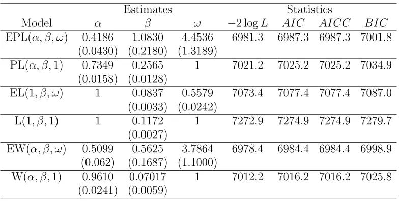
In this section, the EPL distribution is applied to real data in order to illustrate the useful-ness and applicability of the model. We fit the density functions of the exponentiated power Lindley (EPL),power Lindley (PL), exponentiated Lindley (EL) and Lindley (L) distribu-tions. These models are also compared to the exponentiated Weibull (EW) and Weibull (W) distributions. Estimates of the parameters of the distributions, standard errors (in parenthe-ses), Akaike Information Criterion (AIC), Consistent Akaike Information Criterion (AICC), Bayesian Information Criterion (BIC) are given in Table 1 for the first data set, and Table 2 for the second data set.
The first data set is a subset of the breast feeding study from the National Longitudinal Survey of Youth, the complete data set is available in Klein, J.P., Moeschberger, M.L., Survival Analysis: Techniques for Censoring and Truncated Data, 2nd ed., Springer-Verlag New York, Inc., New York (2003). The data set considered here consists of the times to weaning 927 children of white-race mothers who choose to breast feed their children. The duration of the breast feeding was measured in weeks.
The second data set is the Cancer Patients data. The data represents an uncensored data set corresponding to remission times (in months) of a random sample of 128 bladder cancer patients reported in Lee and Wang, (2003). It consists of the observations listed below: 0.08, 2.09, 3.48, 4.87, 6.94, 8.66, 13.11, 23.63, 0.20, 2.23, 3.52, 4.98, 6.97, 9.02, 13.29, 0.40, 2.26, 3.57, 5.06, 7.09, 9.22, 13.80, 25.74, 0.50, 2.46, 3.64, 5.09, 7.26, 9.47, 14.24, 25.82, 0.51, 2.54, 3.70, 5.17, 7.28, 9.74, 14.76, 26.31, 0.81, 2.62, 3.82, 5.32, 7.32, 10.06, 14.77, 32.15, 2.64, 3.88, 5.32, 7.39, 10.34, 14.83, 34.26, 0.90, 2.69, 4.18, 5.34, 7.59, 10.66, 15.96, 36.66, 1.05, 2.69, 4.23, 5.41, 7.62, 10.75, 16.62, 43.01, 1.19, 2.75, 4.26, 5.41, 7.63, 17.12, 46.12, 1.26, 2.83, 4.33, 5.49, 7.66, 11.25, 17.14, 79.05, 1.35, 2.87, 5.62, 7.87, 11.64, 17.36, 1.40, 3.02, 4.34, 5.71, 7.93, 11.79, 18.10, 1.46, 4.40, 5.85, 8.26, 11.98, 19.13, 1.76, 3.25, 4.50, 6.25, 8.37, 12.02, 2.02, 3.31, 4.51, 6.54, 8.53, 12.03, 20.28, 2.02, 3.36, 6.76, 12.07, 21.73, 2.07, 3.36, 6.93, 8.65, 12.63, 22.69. Estimates of the parameters of EPL distribution (standard error in parentheses), Akaike Information Criterion (AIC), Consistent Akaike Information Criterion (AICC) and Bayesian Information Criterion (BIC) are given in Table 8.1 for the first data set and in Table 8.2 for the second data set.
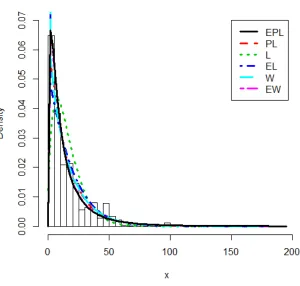
Plots of the fitted densities and the histogram of the data are given in Figure 8.1 for the breastfeeding data, and Figure 8.2 for the cancer patients data.
For the breasfeeding data, the LR statistic of the hypothesis H0: P L(α, β,1) against Ha: EP L(α, β, ω), is λ = 7021.2−6981.3 = 39.9. The p-value is 2.67×10⁻¹⁰ < 0.001. Therefore, we reject H0 in favor of Ha. Thus the EPL distribution performs better than the PL distribution. There is a significant difference between EPL and EL distributions with
λ = 33.9 and p-value=5.80×10⁻⁹ < 0.001. Thus, reject H0: EL vs Ha :EPL in favor of
Ha. A test of H0: L vs Ha : EL shows that λ = 199.5 and p-value=2.68×10−45. Thus, we reject H0 in favor ofHa. To test the hypothesisH0: EP L(α, β, ω) againstHa: EW(α, β, ω), we have λ = 6981.3−6978.4 = 2.9. The p-value is 0.089 >0.05. Thus we fail to reject H0,
For the Cancer Patients data set, the LR statistic for the hypothesis H0: P L(α, β,1)
against Ha: EP L(α, β, ω), is λ= 5.8. The p-value is 0.016<0.05. Therefore, there is a sig-nificant difference between PL and EPL distributions. There is also a sigsig-nificant difference between EPL and EL distributions where λ = 11.7. with a p-value of 6.25×10⁻⁴ <0.001.
There is a significant difference between EL and L distributions with λ = 6.5 and p-value=0.011 < 0.05. A test of H0: EP L(α, β, ω) vs Ha : EW(α, β, ω) shows that λ = 0.5, and p-value=0.480 > 0.05, that there is no significant difference between the two distribu-tions. Based on the values of −2 logL the EPL distribution fits the cancer patients data the best. However, the values of the statistics AIC, AICC and BIC are smaller for the EPL distribution and show that the EPL distribution is a “better” fit for the Cancer Patients data.
8. Concluding Remarks
We have presented and developed the mathematical properties of a new class of distribu-tions called the Exponentiated Power Lindley (EPL) distribution including the hazard and reverse hazard functions, moments, conditional moments, entropies, mean deviations, Lorenz and Bonferroni curves, Fisher information and maximum likelihood estimates. Applications of the proposed model to real data in order to demonstrate the usefulness and applicability of the class of distributions are also presented.
Table 8.1. Estimates of Models for Breastfeeding Data
Estimates Statistics
Model α β ω −2 logL AIC AICC BIC
EPL(α, β, ω) 0.4186 1.0830 4.4536 6981.3 6987.3 6987.3 7001.8 (0.0430) (0.2180) (1.3189)
PL(α, β,1) 0.7349 0.2565 1 7021.2 7025.2 7025.2 7034.9 (0.0158) (0.0128)
EL(1, β, ω) 1 0.0837 0.5579 7073.4 7077.4 7077.4 7087.0 (0.0033) (0.0242)
L(1, β,1) 1 0.1172 1 7272.9 7274.9 7274.9 7279.7
(0.0027)
EW(α, β, ω) 0.5099 0.5625 3.7864 6978.4 6984.4 6984.4 6998.9 (0.062) (0.1687) (1.1000)
Figure 8.1. Plot of the fitted densities for the Breastfeeding Data
Table 8.2. Estimates of Models for Cancer Patients Data
Estimates Statistics
Model α β ω −2 logL AIC AICC BIC
EPL(α, β, ω) 0.5663 0.8191 2.7684 820.9 826.9 827.1 835.4 (0.1017) (0.3116) (1.2903)
PL(α, β,1) 0.8302 0.2943 1 826.7 830.7 830.8 836.4 (0.0472) (0.0370)
EL(1, β, ω) 1 0.1649 0.7336 832.6 836.6 836.7 842.3 (0.0166) (0.0912)
L(1, β,1) 1 0.1960 1 839.1 841.1 841.1 843.9
(0.0123)
EW(α, β, ω) 0.6544 0.4537 2.7960 821.4 827.4 827.6 835.9 (0.1347) (0.2399) (1.2635)
References
[1] A. Asgharzedah, H.S. Bakouch and H. Esmaeli, Pareto Poisson-Lindley Distribution with Applications, Journal of Applied Statistics, 40(8)(2013).
[2] R.M. Corless, G.H. Gonnet, D.E.G. Hare, D.J. Jeffrey and D.E. Knuth, On the Lambert W function. Advances in Computational Mathematics, 5(1996), 329-359.
[3] M.E. Ghitany, B. Atieh and S. Nadarajah, Lindley Distribution and Its Applications, Mathematics and Computers in Simulation, 78(4)(2008), 493-506.
[4] M.E. Ghitany, D.K. Al-Mutairi, N. Balakrishnan and L.J. Al-Enezi, Power Lindley distribution and associated inference, Computational Statistics and Data Analysis, 64(2013), 20-33.
[5] I.S. Gradshteyn, I.M. Ryzhik, Tables of Integrals, Series, and Products, seventh ed. Academic Press, New York, 2007.
[6] J.P. Klein, M.L. Moeschberger, Survival Analysis: Techniques for Censoring and Truncated Data, 2nd ed., Springer-Verlag New York, Inc., New York, 2003.
[7] D.V. Lindley, Fiducial distributions and Bayes theorem, Journal of the Royal Statistical Society, Series B 20(1958), 102-107.
[8] S. Nadarajah, H.S. Bakouch and R. Tahmasbi A Generalized Lindley Distribution, Sankhya B, 73(2011), 331-359.
[9] A. R´enyi, On measures of entropy and information, Proceedings of the 4th Berkeley Symposium on Mathematical Statistics and Probability, vol. I, University of California Press, Berkeley, (1961), 547-561.
[10] E.A. Shannon, A Mathematical Theory of Communication, The Bell System Technical Journal, 27(10)(1948), 379-423.
[11] E.A. Shannon, A Mathematical Theory of Communication, The Bell System Technical Journal, 27(10)(1948), 623-656.
[12] M. Shaked and J.G. Shanthikumar, Stochastic Orders and Their Applications, Academic Press, New York, 1994.
[13] M. Sankaran, The Discrete Poisson-Lindley Distribution, Biometrics, 26(1)(1970), 145-149.