Sensorless Fuzzy Sliding Mode Speed Controller for DTC of Induction Motor based on DSVM

ISSN 1991-8178

Corresponding Author: Ahmed Massoum, Faculty of technology, Department of electrical engineering, Djillali Liabes

Sensorless Fuzzy Sliding Mode Speed Controller for DTC of Induction Motor

based on DSVM

1_{Ahmed Massoum,} 2_{Abdelkader Meroufel,} 1_{Abdelhakim Hammoumi,} 2_Patrice.Wira

1_{Faculty of technology, Department of electrical engineering, Djillali Liabes University, Sidi Bel}

Abbes, Algeria

2_{MIPS-TROP Laboratory, Haute Alsace University, Mulhouse, France}

Abstract: Direct Torque Control (DTC) is known to produce quick and robust response in ac drives. However, in the classical DTC scheme, due to the limited number of the VSI voltage vectors, large and small errors can not be distinguished. In fact, the switching vectors chosen for large errors are the same as those chosen for small errors. This problem appears in fluctuations form, during steady state in torque, flux, and current. They are reflected in flux and torque estimation, and also in speed response. In this paper, a DTC based on Discrete Space Vector Modulation (DSVM) for Induction Motor (IM) sensorless drive with Fuzzy Sliding Mode Speed Controller (FSMSC) is presented. The proposed control system is able to reduce the torque, flux, current, and speed pulsations during steady state. The rotor speed and stator flux are estimated by the Model Reference Adaptive System (MRAS) scheme which is determined from measured terminal voltages and currents. The speed estimator is then applied to sensorless Discrete Space Vector Modulation-Direct Torque Control (DSVM-DTC) of IM drive system. The FSMSC is used in order to increase the performances and the robustness of the speed closed loop. The performance of the drive system has been verified by simulation tests, and good results have been achieved in both steady-state and transient operating conditions.

Key words: IM, DTC, DSVM-DTC, MRAS, Sensorless, FSMSC.

INTRODUCTION

number of voltage space vectors can be synthesized compared to those used in the basic DTC technique. The increased number of voltage vectors allows the definition of more accurate switching tables in which the selection of voltage vectors is made according to the rotor speed, the flux error and the torque error. The advantage of using the DSVM technique is that one can choose among 19 voltage vectors instead of 5 of the basic DTC. The DSVM can produce more voltage vectors which if properly applied produce less ripple. To achieve this, the torque hysteresis has 5 levels instead of two. The look-up table in this case has four input variables; flux and torque hysteresis state, sector number and speed voltage. Since the system chose voltage vectors depending on the emf, each speed region uses different switch tables. When the system operates in the high speed region two switch tables for each sector are used. Because the emf introduces an asymmetry, the switch tables also become asymmetric. Hence, different tables must be used for positive and negative rotational directions. The DSVM-DTC achieves a sensible reduction of torque ripple, without increasing the complexity of conventional DTC. However, simple PI based DSVM-DTC controller cannot handle dynamically changing situations like parameter uncertainties, nonlinearities in the inverter and motor, and inadequate rejection of internal disturbances and load changes. This is why the strategies and methods of robust control have been paid close attention to. The sliding mode controller (SMC) has been suggested to achieve robust performance against parameter variations and load disturbances. It also offers a fast dynamic response, stable control system and easy hardware-software implementation. On the other hand, this control method offers some drawbacks associated with the large torque chattering that appears in steady state, which may excite mechanical resonance. In order to reduce the system chattering, a SMC with fuzzy sliding surface were proposed. The fuzzy logic controller (FLC) is not dependent on the accurate mathematical model of the system. It is based on ‘IF…THEN’ rules and experiences of human beings. In this paper, by means of the advantage of SMC and FLC, a synthetic control scheme is presented. The fuzzy sliding mode speed controller (FSMSC) is designed for the speed regulation of DSVM-DTC- IM fed by a voltage source inverter. In conventional speed control of DTC the actual value of rotor speed is required. The controller receives the signals of rotor speed from the speed sensors. Unfortunately, the accuracy of the control system will decrease with the appearance of noises, causing low reliability. Furthermore, the conventional sensors make the higher cost; increase the complexity of the systems because of noise filtering. The filtering will help to improve the quality of feedback speed; however, additional digital filters require higher computing capacities for faster signal processing and transmission. Therefore, they mount additional costs on the overall systems.

Recently, many researchers have been carried out for the design of speed sensorless control schemes. In these new schemes the speed is obtained from the determined stator voltages and measured stator currents instead of using a sensor. Sensorless techniques are presented, an open loop and a close-loop (MRAS) scheme, which can overcome the necessity of the speed sensor. To evaluate the usefulness of the proposed method, we compare it to other controllers. The Modeling of DSVM-DTC-IM based drive system is presented in Matlab/Simulink models in order to study the performance of the drive system under steady state and dynamic conditions during starting, and speed reversal and load perturbations. The simulation results show that the proposed method control can achieve very robust and satisfactory performance.

Principle Of Dtc:

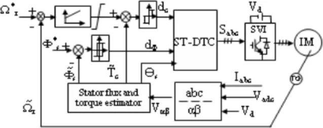
The block diagram of classical DTC scheme is shown in fig.1. The stator flux and torque magnitudes are controlled by two independent hysteresis controllers. The selection of the appropriate voltage vector is based on the Switching Table (ST) given in Table1.

Fig. 1: Block diagram of simulated ST-DTC with speed controller

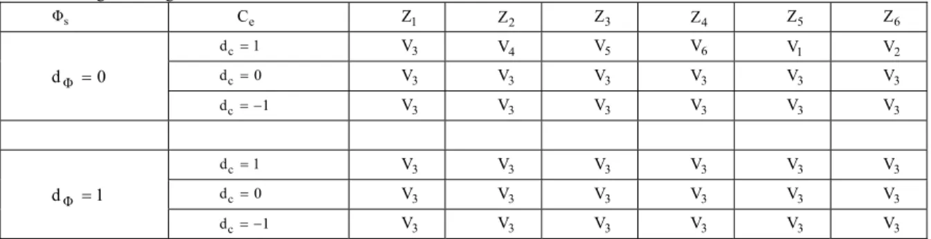
Table 1: Basing switching

s

Φ C_e Z₁ Z₂ Z₃ Z₄ Z₅ Z₆

0 d_Φ 

1

d_c V₃ V₄ V5 V6 V1 V2

0

d_c V₃ V₃ V₃ V₃ V₃ V₃

1

d_c V3 V3 V3 V3 V3 V3

1 d_Φ 

1

d_c V₃ V₃ V₃ V₃ V₃ V₃

0

d_c V₃ V3 V3 V3 V3 V3

1

d_c V3 V3 V3 V3 V3 V3

(i=1,2,…,6), , denote stator flux position, torque error and stator flux error respectively.

Fig. 2: Voltage vectors obtained by using DSVM with three equal intervals per cycle

2.1. Stator Flux Control:

Stator flux estimation based on voltage model is estimated by using equation: dt

) I R V (

Φ s s s

t

0

s 



During the switching interval, when stator resistance drop is neglected in high speed operating condition, the relationship between the voltage vectors and flux variation is given by:

e s s

s(k+1)≈Φ (k)+VT

Φ or ΔΦ_s(k)V_sT_e (2)

The instantaneous flux speed is only governed by voltage vector amplitude given in (2). The values of and are calculated by using the DC link voltage , the inverter switching states , , and , and the motor line currents . It can be proven that the space vector of the rotor flux is related to that of the stator flux by the following equation in the s-domain with a first-order delay equation.

s r s m

r _1+sδT Φ

L / L =

Φ (3)

The stator flux angle is calculated by )

Φ / Φ arctan( =

θ_{s qs ds} (4)

2.2. Electromagnetic Torque Control:

(

)

r

e _{L L} Φ I -Φ I

pM 2 3 =

T ₍₅₎ 3. Dsvm-Dtc Strategy:

In this paper the number of voltage vectors is increased using a standard VSI topology and introducing a simplified space vector modulation technique. According to the principle of operation, new voltage vectors can be synthesized by applying, at each cycle period, several voltage vectors for prefixed time intervals. In this way a sort of DSVM is employed which requires only a small increase of the computational time [D. Casadei et al., 2000]. The number of the voltage vectors which can be generated is directly related to the numbers of time intervals by which the cycle period is subdivided. Higher the numbers of voltage vectors lower the amplitude of current and torque ripple. However, a high number of voltage vectors require the definition of new and more complex switching tables. A good solution should be defined as a compromise between the perfect ripple compensation and the complexity of the voltage vector selection strategy. It has been verified that subdividing the cycle period in three equal time intervals leads to a substantial reduction of torque and current ripple without the need of too complex switching tables. Using the DSVM technique, with three equal time intervals, 19 voltage vectors can be used, as represented in fig.6. The black dots represent the ends of the synthesized voltage vectors. As an example, the label "332" denotes the voltage vector which is synthesized by using the voltage space vectors V3, V3 and V2, each one applied for one third of the cycle period. ‘ Z’ denotes a zero voltage

vectorV0 orV7 (D. Ocen et al., 2006; Xin Wei et al., 2004).

The voltage vector selection strategy should be defined using all the 19 voltage vectors on the basis of the criteria discussed in the preceding Section. In particular it has been verified a large influence exerted by the dynamic emf rΦs. So this quantity together with the actual outputs of flux and torque comparators are

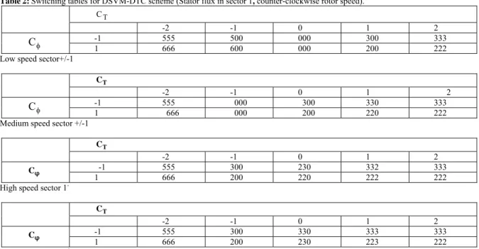
assumed as input variable to the switching tables. The results of the analysis can be summarized in seven switching tables for the stator flux lying in sector 1. For sake of simplicity, only the four related to counterclockwise angular speed are given in Tab.2.

Fig. 3: Speed range subdivision, pu of the rated voltage

Table2:Switching tables for DSVM-DTC scheme (Stator flux in sector 1, counter-clockwise rotor speed).

T C

-2 -1 0 1 2



C -1 ₁ 555₆₆₆ 500 ₆₀₀ 000 ₀₀₀ 300 ₂₀₀ 333 ₂₂₂

Low speed sector+/-1

T C

-2 -1 0 1 2



C -1 ₁ 555 ₆₆₆ 000 ₀₀₀ 300 ₂₀₀ 330 ₂₂₀ 333₂₂₂

Medium speed sector +/-1

T C

-2 -1 0 1 2

φ

C -1 555 300 230 332 333

1 666 200 220 222 222

High speed sector 1-

T C

-2 -1 0 1 2

φ

C -1 555 300 330 333 333

1 666 200 230 223 222

It is assumed the stator flux is lying in sector 1. Then the 19 available voltage vectors are denoted according to the map given in fig.2. The first switching table is valid for low speed operation, the second for medium speed and the last two for high speed. The speed ranges are defined with reference to the value assumed by the dynamic emf _rΦ_s, as represented in fig.3.

In each table the synthesized voltage vectors are selected by a two-level hysteresis band for the flux, and a five-level hysteresis band for the torque. The torque hysteresis comparator operates according to figure 4. With reference to this last, it should be noted that levels -1, 0 and +1 are involved in steady state operating conditions and for limited torque variation demand. In these operating conditions the 4 voltage vectors which produce limited torque variations are selected. Levels -2 and +2 are involved only during high dynamic transients.

In the high speed range two switching tables have been defined, each one valid for half a sector (1+ _{and 1}- _).

This means that the argument of the stator flux vector has to be estimated with a resolution of corresponding to a 12 sector angular representation. Two switching tables are necessary at high speed to fully utilize the available voltage vectors. In order to explain how the synthesized voltage vectors are selected at high speed, we assume for the machine a counter-clockwise rotation and a torque increase demand. In this case, the 4 voltage vectors can be employed, i.e. “333”, “332”, “223” and “222”. Depending on whether the flux has to be reduced or increased, the first two vectors or the last two vectors respectively should be selected.

So, if we have to force the flux to decrease we can choose between “333” and “332”. For the last step we have to verify the position of the flux vector. If the flux is in sector 1+ _{the vector “333” is selected, while with}

the flux in sector 1- _{it is opportune to select “332”. It should be noted that it is not possible to apply these}

selection criteria in the medium and low speed range because the number of available voltage vectors is not high enough.

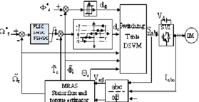
Dsvm-Dtc-Im Scheme:

The functional blocks of a DSVM-DTC system is shown in fig.5. Stator flux and torque are controlled using respectively a two level and five level hysteresis comparators. Their status, together with the rotor speed and the stator flux switching sector, are used to select the voltage vector to be applied to the IM.

Fig. 5: Block diagram of simulated Sensorless speed controller DSVM-DTC-IM scheme

Fig. 4: Proposed five levels torque comparator

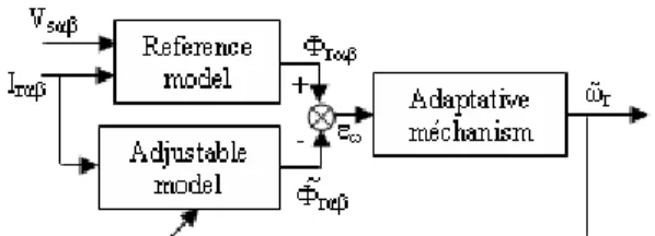
Fig. 6: Classical MRAS structure for speed estimation

Rotor Speed Estimation By Mras Technique:

Sensorless drives are becoming more and more important as they can eliminate the speed sensor maintaining accurate response. Monitoring only the stator current and stator voltages, it is possible to estimate the necessary control variables. The observer type used here is a MRAS (R. Kumar et al., 2006; F.J.lin et al., 1999). The basic scheme of the MRAS configuration is given in Fig.6. The scheme consists of two models; reference and adjustable ones and an adaptation mechanism. The block “reference model” represents voltage model which is independent of speed. The block “adjustable model” is the current model which is using speed as a parameter. The block “adaptation mechanism (PI controller)” estimates the unknown parameter using the error between the reference and the adjustable models and updates the adjustable model with the estimated parameter until satisfactory performance is achieved. Since the MRAS is a close-loop system, the accuracy can be increased. However, the models contain pure integrators which cause estimation error due to unknown initial condition and estimation drift due to offset in the measured currents. To avoid the problem, low-pass filters are used (R. Kumar et al., 2006; F.J.lin et al., 1999).

5.1. Reference Model Equations:

The reference rotor flux components obtained from the reference model are given by:

 







   

 





m r

r _L V R V dt L I

L

Φ (6)

5.2. Adaptive Model Equations:

The rotor flux components obtained from the adaptive model are given by:

 

 

 

T L Φ~ T

1

Φ~ s

r m r r r

r  

  

  

    

 

 

 _{ }

 (7)

5.3. Error Between Two Models:

estimated speed can be given as:





 

 Φ_r Φ~_r -Φ_r Φ~_r (8)

dt k k ~

i p

r  



 (9)

Fuzzy Sliding Mode Control:

FSMC is at present employed as an alternative to develop controller for systems that cannot be precisely modelled and whose parameters vary (A. Meroufel et al., 2008; S.M. Gadoue et al., 2007; S. Jabeur et al., 2005). To design a sliding mode speed controller for the induction motor DTC-SVM drive, consider the mechanical equation:

e r r f

r _p T T

K p

J_{    }

 (10)

Where _ris the rotor speed in electrical rad/s, rearranging to get:

r r f e

r _JT

p -J K -T J

p _



 ₍₁₁₎

Considering aΔ and bΔ as bounded uncertainties introduced by system parameters J and Kf , (11) can

be rewritten as [11]:



 



r  aΔa bΔbT cT

 ₍₁₂₎

where _J

K a f _,

J p b _,

J p -c

Defining the state variable of the speed error as:

 

 

 

e _r *_{r (13)}

Combining (12) with (13) and taking the derivative of (13) yields

 

 



 



e   _e ₍₁₄₎

where d(t)is the lumped uncertainty defined as:

 

 

c T b

b

Δ

t b

a

Δ

t

d     (15)

and

* e

e(t) T (t) _ba

T    (16)

Defining a switching surface s(t) from the nominal values of system parameters aand b:

    

_

  

0

d e bk a -t e t

s ₍₁₇₎

Such that the error dynamics at the sliding surface s(t)s(t)0 will be forced to exponentially decay to zero, then the error dynamics can be described by:

  

  

e   (18)

 

 

 

T_e   (19)

where  is known as hitting control gain used to make the sliding mode condition possible and the sign function can be defined as:

    

 

  

0 s if 1

0 s if 0

0 s if 1 ) s (

sign (20)

The final electromagnetic torque command * e

T of the output of the sliding mode speed controller can be obtained by directly substituting (16) into (19). Basically, the control law for T_e* is divided into two parts: equivalent control U_eqwhich defines the control action when the system is on the sliding mode and switching part U_s which ensures the existence condition of the sliding mode. If the friction Bis neglected expressions for

eq

U and U_s can be written as:

)) t ( s ( sign U

) t ( ke U

s eq

  



(21)

To guarantee the existence of the switching surface consider a Lyapunov function: )

t ( s 2 1 ) t (

V  2 (22)

Based on Lyapunov theory, if the function V(t) is negative definite, this will ensure that the system trajectory will be driven and attracted toward the sliding surface s(t)and once reached, it will remain sliding on it until the origin is reached asymptotically (L.M. Gnesiak and B. Ufnalski, 2004; F. Barrero et al., 2002; V.I.Utkin, 1993; M. Depenbrock, 1988 A). Taking the derivative of (22) and substituting from the derivative of (17):

 





) t (

V        (23)

Substitute from (6) into (15):

 

 





s   _e   _e (23)

Using (11) gives

 

 



s      (24)

To ensure that (17) will be always negative definite, the value of the hitting control gain β should be designed as the upper bound of the lumped uncertainties d(t), i.e.

) t ( d 

 (25)

However, it is difficult practically to estimate the bound of uncertainties in (17). Therefore the hitting control gain βhas to be chosen large enough to overcome the effect of any external disturbance. Therefore the speed control law defined in (19) will guarantee the existence of the switching surface s(t) in (17) and when the error function e(t) reaches the sliding surface, the system dynamics will be governed by (18) which is always stable. Moreover, the control system will be insensitive to the uncertainties Δa , Δband the load disturbance

r

C . The use of the sign function in the sliding mode control (19) will cause high frequency chattering due to the discontinuous control action which represents a severe problem when the system state is close to the sliding surface (A, Sabanovic and F. Bilalovic, 1993; L. Tang et al, 2004).

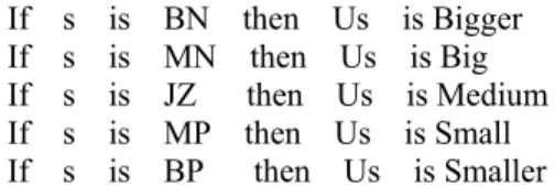
replaced by a fuzzy inference system in order to avoid the chattering phenomenon. The FSMC is a single input single output fuzzy logic controller. It is constructed from the following format ‘IF….THEN’ rules or equivalently. The max-min composition is chosen as the inference method. The crisp output is obtained by the center of the area defuzzifier. The If-Then rules of the fuzzy logic controller can be written as (B. Robyns et al., 2000; S. A. Mir et al, 1994).

If s is BN then Us is Bigger If s is MN then Us is Big If s is JZ then Us is Medium If s is MP then Us is Small If s is BP then Us is Smaller

where BN: Big Negative; MN: Medium Negative; JZ: Just Zero; MP: Medium Positive; BP: Big Positive. The membership functions for the input and output of the FL controller are obtained by trial error to ensure optimal performance and are shown in Figure 3.

Simulation Result And Discussion:

To study the performance of the sensorless speed control, FSM Controller of speed and SVM_DTC strategy, the simulation of the system was conducted using Matlab/Simulink and Fuzzy logic Toolbox. The torque and flux hysteresis bands of 0.2Nm and 0.01Wb respectively were used to give a switching frequency. The induction motor used in this case study is a 1.5kw, 380/220V, four poles, 50Hz; with the following parameters: Rs = 4.85, Rr = 3.805, Ls = 0.274H, Lr = 0.274H and Lm = 0.258H.

The system has the following mechanical parameters: J = 0.031 kg.m2_{, f}

r = 0.000114 Nm.s-1

The block ‘PWM Inverter’ is a six IGBT-diode bridge inverter with 480 V DC voltage source.

From fig.7, it has been verified that in the case DSVM-DTC scheme allows the torque and the flux ripple to be reduced with an increase of the inverter switching frequency. The behavior of the two DTC schemes in step torque shows a good torque time response.

0 0.05 0.1 0.15 0.2 0

5 10

t(sec)

T

o

rq

u

e

(N

m

)

Classical DTC

0 0.05 0.1 0.15 0.2 0

5 10

DSVM-DTC

t(sec)

T

o

rq

u

e

(N

m

)

0 0.05 0.1 0.15 0.2 0

0.5 1

t (sec)

S

tat

or

f

lu

x

(

W

b

)

0 0.05 0.1 0.15 0.2 0

0.5 1

t (sec)

S

tat

or

f

lu

x

(

W

b

)

0.025 0.03 0.035 0.04 0.045 9.5

10 10.5

0.025 0.03 0.035 0.040.045 9.5

10 10.5

0.06 0.08 0.1 0.98

1

0.06 0.08 0.1 0.98

1

Fig. 7: Simulation results with classical DTC scheme and with DSVM-DTC scheme

0 0.5 1 1.5 2 2.5 -50

0 50 100 150

t (sec)

S

p

e

ed (

ra

d

/s

ec

)

0 0.5 1 1.5 2 2.5

-30 -20 -10 0 10

t (sec)

T

o

rq

u

e

(N

m

)

0 0.5 1 1.5 2 2.5

0 0.5 1

t (sec)

F

lux

(

W

b)

Wref Wr West

Electromagnetic torque

Stator flux

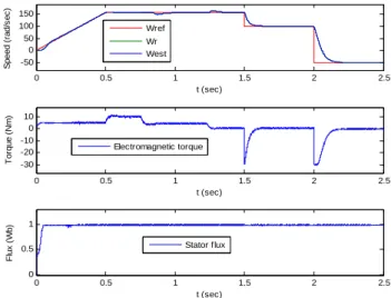
Fig. 8: Simulation results of speed estimator (West), electromagnetic torque and stator flux

The rotor speed (Wr) and the estimated speed (West) follow-up to the reference speed (Wref) in spite of the abrupt command change.

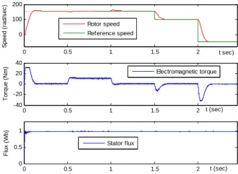
From fig.9 and fig.10 it can be seen that the speed response presents better tracking characteristics. The external disturbance (load torque) on the speed response is rejected rapidly. Better decoupled properties are obtained and fluxes track the desired fluxes precisely.

From the system responses given in fig. 11 and fig.12 for SMSC and FSMSC the mechanical speed tracks the reference speed without overshoot, with zero steady state error and with an instantaneously perturbation reject. The results show that high precision tracking can be achieved using the speed SMSC and FSMSC in spite of large parameter variations.

0 0.5 1 1.5 2

0 100 200

t (sec)

S

pee

d (

rad

/s

ec

)

0 0.5 1 1.5 2

-40 -20 0 20 40

t (sec)

To

rq

u

e

(

N

m

)

0 0.5 1 1.5 2

0 0.5 1

t (sec)

F

lux

(

W

b)

Rotor speed Reference speed

Electromagnetic torque

Stator flux

0 0.5 1 1.5 2 0 100 200 t sec) S p e ed ( ra d /s e c )

0 0.5 1 1.5 2

-40 -20 0 20 40 t (sec) T o rque ( N m )

0 0.5 1 1.5 2

0 0.5 1 t (sec) F lux ( W b) Rotor speed Reference speed Electromagnetic torque Stator flux

Fig. 10: Simulation response with Fuzzy logic speed variations for DSVM-DTC

0 0.5 1 1.5 2

0 100 200 t (sec) Sp eed (r a d /s ec )

0 0.5 1 1.5 2

-40 -20 0 20 40 t (sec) T o rque (N m )

0 0.5 1 1.5 2

0 0.5 1 t (sec) Fl u x ( W b ) Rotor speed Reference speed Stator flux Electromagnetic torque

Fig. 11: Simulation reponse with Sliding mode speed variations for DSVM-DTC

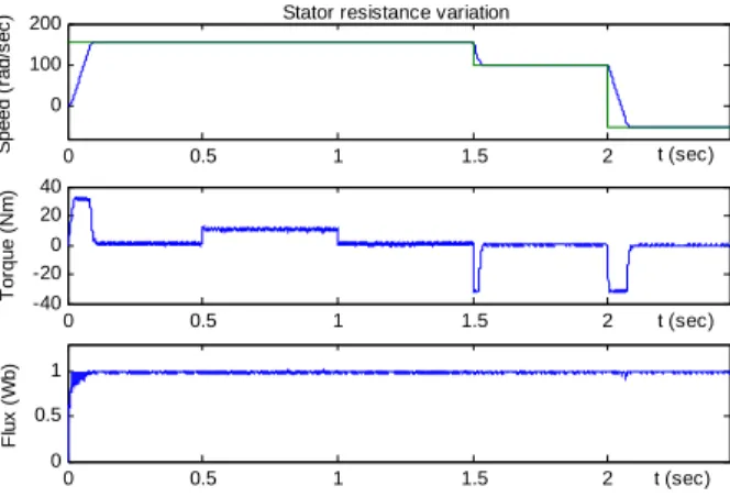
Robustness tests:

In order to test robustness of the proposed control, we have studied stator resistance and inertia variations. Stator resistance variation:

The sensitivity of stator resistance is investigated because its variation greatly affects the performance of the DTC drive (fig.13)

0 0.5 1 1.5 2

0 100 200 t (sec) S p e ed ( rad /s ec )

0 0.5 1 1.5 2

-40 -20 0 20 40 t (sec) To rq u e (N m )

0 0.5 1 1.5 2

Fig. 12: Simulation reponse with Fuzzy Sliding mode speed variations for DSVM-DTC

0 0.5 1 1.5 2

0 100

200 Stator resistance variation

t (sec)

S

p

e

ed (

ra

d/

s

e

c

)

0 0.5 1 1.5 2

-40 -20 0 20 40

t (sec)

To

rq

u

e

(N

m

)

0 0.5 1 1.5 2

0 0.5 1

t (sec)

F

lux

(

W

b)

Fig. 13: Speed, torque and stator flux responses with stator resistance under FSMC

FSMC shows the robustness of the controller under the stator resistance variation and the load torque disturbance.

Inertia variation:

It is shown from fig.14 that the proposed drive can follow the reference speed accurately due to the robustness of the FSMC. We remark that the time speed response increases with inertia (1.5 Jn) and the other performances are maintained.

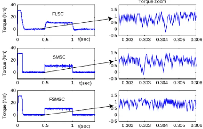
Ripple reduction :

The influence of chattering is investigated through a comparison between FLSC, SMSC and FSMSC applied to DSVM-DTC scheme (fig.15).

From the analysis of these results, we establish the following remark. The amplitude of the torque ripples in steady state is gradually reduced with FSMSC.

Conclusion:

From simulation results it was shown that the proposed FSMSC for DSVM-DTC scheme is robust to external variations and has presented satisfactory performances in speed response (no overshoot, zero steady state error and good tracking reference speed). The robustness test has shown that it is insensitive to rotor resistance variation and inertia variation. The decoupling between the flux and the torque (speed) is maintained with regard to parameter variations and external load disturbance. The chattering phenomenon is decreased in torque when compared to other controllers. The FSMSC-DSVM-DTC scheme has very interesting dynamic performances and provides improvement in ripple reduction in torque. So a lower harmonic content in the stator currents will reduce torque fluctuations, current harmonics, vibrations, noise and hot in the motor are also reduced.

0 0.5 1 1.5 2

0 100

200 Inertia variation

t (sec)

S

peed (

rad/

s

e

c

)

0 0.5 1 1.5 2

-40 -20 0 20 40

t (sec)

T

o

rque (

N

m

)

0 0.5 1 1.5 2

0 0.5 1

t (sec)

F

lux

(

W

Fig. 14: Speed, torque and flux responses with rotor inertia J=1.5*Jn

0 0.5 1

0 20 40

FLSC

t(sec)

To

rq

u

e

(

N

m

)

0 0.5 1

0 20 40

SMSC

t(sec)

T

o

rq

u

e

(N

m

)

0.302 0.303 0.304 0.305 0.306 -0.5

0 0.5 1 1.5

0 0.5 1

0 20 40

FSMSC

t(sec)

T

o

rque

(

N

m

)

0.302 0.303 0.304 0.305 0.306 -0.5

0 0.5 1 1.5

0.302 0.303 0.304 0.305 0.306 -0.5

0 0.5 1 1.5

Torque zoom

Fig. 15: Torque response with zoom in steady state

REFERENCES

Barrero, F., A. Gonzalez, A. Torralba, E. Galvan, L.G. Franquelo, 2002. Speed control of induction motors using a novel fuzzy sliding mode structure. IEEE Trans. Fuzzy Syst, 10(3): 375-383.

Casadei, D., G. Sera and A. Tani, 2000. Implementation of a direct control algorilhm for induction motors based on discrete space vector modulation, IEEE Trans. Power Elecrron., IS(4): 769-777.

Depenbrock, M., 1988. Direct self-control (DSC) of inverter-fed induction machine. IEEE Trans. Power Electronics, 3(4): 420-429.

Gadoue, S.M., D. Giaouris and J.W. Finch, 2007. Genetic Algorithm Optimized PI and Fuzzy Sliding Mode Speed Control for DTC Drives. Proceedings of the World Congress on Engineering, pp: 475-480.

Gnesiak, L.M., B. Ufnalski, 2004. Neural Stator Flux Estimator with Dynamical Signal Preprocessing. IEEE Conference. AFRICON- pp: 1137-1142.

Gupta, R.A., R. Kumar, A.K. Bansal, 2006. Artificial intelligence applications in Magnet Brushless DC Motor Drive. IEEE conference. (IECON-) pp: 649-654.

Habetler, T.G., F. Profumo, M. Pastorelli and L.M.Tolbert, 1992. Direct torque control of induction machines using space vector modulation. IEEE Trans. Ind. Appl., 28(5): 1045-1053.

Jabeur, S., C.B., F. Fnaiech, 2005. DTFC and DTNFC: Two Intelligent Techniques for Induction Motors Torque Control. Industrial Electronics, Proceedings of the IEEE International Symposium, pp: 131-138.

Kumar, R., S.V. Radmanaban, 2006. An Artificial Neural Network Based Rotor Position Estimation for Sensorless Permanent Magnet Brushless DC Motor Drive. IEEE Industriel Electronics, IECON, pp: 649-654 .

lin, F.J., R.J. Wai and P.C. Lin, 1999. Robust speed sensorless induction motor drive . IEEE, Trans, Aerosp Electron. Syst, 35(2): 566-578.

Meroufel, A., A. Massoum and P. Wira, 2008. A Fuzzy Sliding Mode Controller for a Vector Controlled Induction Motor. Industrial Electronics, ISIE 2008. IEEE International Symposium on , pp: 1873-1878.

Mir, S.A., M.E. Elbuluk and D.S. Zinger, 1994. Fuzzy implementation of direct self-control of induction machines. IEEE Trans. Ind. Appl., 30(3): 729-735.

Ocen, D., L. Romeral, J.A. Ortega, J. Cusido and A. Garcia, 2006. Discrete space vector modulation applied on a PMSM motor.Proc. EPEPEMC, pp: 320-325.

Robyns, B., F. Berthereau, J.-P. Hautier, H. Buyse, 2000. A fuzzy-logic-based multimodel field orientation in an indirect FOC of an induction motor. IEEE Trans. on Industrial Electronics, 47(2): 380-388.

Sabanovic, A. and F. Bilalovic, 1993. Sliding mode control of AC drives. IEEE, Trans on Ind.Appl, IA-25(1): 70-75.

Takahashi, I., N. Toshihiko, 1986. A New Quick-Response and High Efficiency Contro l Strategy of an Induction Motor. IEEE Transactions on Industry Applications, IA(22): 820-827.

Tang, L., L. Zhong, M.F. Rahman, and Y. Hu, 2004 . A novel direct torque control for interior permanent magnet synchronous machine drive system with low ripple in flux and torque and fixed switching Frequency. IEEE Trans.Power. Electron, 19(22): 346-354.