doi:10.1093/biostatistics/kxw015
Estimation of a partially linear additive model for data
from an outcome-dependent sampling design
with a continuous outcome
ZIWEN TAN, GUOYOU QIN∗
Department of Biostatistics, School of Public Health and Key Laboratory of Public Health Safety, Fudan University, Shanghai 200032, China
HAIBO ZHOU
Department of Biostatistics, University of North Carolina at Chapel Hill, Chapel Hill, NC 27599, USA
SUMMARY
Outcome-dependent sampling (ODS) designs have been well recognized as a cost-effective way to enhance study efficiency in both statistical literature and biomedical and epidemiologic studies. A partially linear additive model (PLAM) is widely applied in real problems because it allows for a flexible specification of the dependence of the response on some covariates in a linear fashion and other covariates in a non-linear non-parametric fashion. Motivated by an epidemiological study investigating the effect of prenatal polychlorinated biphenyls exposure on children’s intelligence quotient (IQ) at age 7 years, we propose a PLAM in this article to investigate a more flexible non-parametric inference on the relationships among the response and covariates under the ODS scheme. We propose the estimation method and establish the asymptotic properties of the proposed estimator. Simulation studies are conducted to show the improved efficiency of the proposed ODS estimator for PLAM compared with that from a traditional simple random sampling design with the same sample size. The data of the above-mentioned study is analyzed to illustrate the proposed method.
Keywords: Design-based sampling; Empirical likelihood; Polychlorinated biphenyls; Semi-parametric model.
1. INTRODUCTION
Epidemiologists and biostatisticians are now paying more attention to the outcome-dependent sampling (ODS) design recognizing that it is a cost-effective way to improve study efficiency. A general ODS scheme, e.g. the case–control study inCornfield(1951), is a retrospective sampling scheme where the primary exposure or covariates are only observed on some subsets of the study population with a probabil-ity depending on the value of the outcome variable which can be either continuous or discrete. The principle idea of such a design is to concentrate resources where there is the greatest amount of information, thus
∗To whom correspondence should be addressed.
c
making it more appealing than the traditional simple random sampling (SRS), to provide increased statis-tical power or equivalently, a reduced sample size given a fixed budget.
The ODS design is especially attractive when considering the high cost of assessing the exposure vari-able and the easy availability of the outcome. For example, in a recent epidemiological study employing an ODS design (Grayand others,2005), investigators were interested in studying how in utero exposure to polychlorinated biphenyls (PCBs), which is represented by maternal third trimester serum PCB lev-els, is related to the offspring’s intelligence quotient (IQ) at 7 years of age. The study subjects are chil-dren born into the Collaborative Perinatal Project (CPP); a prospective cohort was designed to identify determinants of a wide variety of neurological outcomes and birth defects (Niswander and Gordon,1972). Because of the great expense associated with the blood serum assay to obtain the PCB levels of all 43 628 eligible children from the 55 908 pregnancies recruited from 12 U.S. study centers from 1959 to 1965 (Longneckerand others,2001), the investigators chose to measure the PCB exposure for a sample that was assembled in an ODS way based on the observed IQ scores. That is, treating the eligible 43 628 chil-dren as a known population, an overall simple random sample of 1256 subjects and an additional 207 children from those with IQ scores either one or more standard deviations below or above the mean were included in the sample.
For analysis of data obtained through such a complex ODS design as described above, the usual methods like maximum likelihood, assuming identically and independently distributed data, and ordi-nary least squares, would derive inconsistent estimations (Holtand others,1980). Unlike the case–control study where the sampling scheme can be ignored as the underlying model is logistic, the analysis for data from an ODS design with a continuous response must take into account that the ODS design is a biased sampling scheme to avoid biased estimates of the regression parameters. Several methods have been developed for this purpose. Commonly used methods include the weighted estimating equation approach byHorvitz and Thompson(1952), where the weights are inversely proportional to the probabil-ity of being sampled (inverse probabilprobabil-ity weighting), and another weighted pseudo-likelihood method by
Holtand others(1980), requiring a correct specification of all the underlying distributions. These methods, however, only account for the sampling scheme in an approximate way.Zhouand others(2002) proposed a more efficient semi-parametric empirical likelihood method in which no distribution of the exposure vari-able was specified and the biased sampling design was more precisely reflected in the likelihood function. A pseudo-score estimation method was also considered byChatterjeeand others(2003) for ODS data, as well as the estimated likelihood method proposed byWeaver and Zhou(2005).
Recently, an increasing number of papers focusing on the efficiency gain and application of ODS designs, development of ODS designs and model fitting for the ODS data have been published. For example, in the framework of linear models, Zhouand others (2007) investigated the efficiency gain of the ODS designs under a wide range of the exposure distributions and illustrated the application of the ODS designs through 3 epidemiological real data.Xu and Zhou(2012) proposed a mixed regression model for a cluster base of a two-stage outcome-auxiliary-dependent sampling design with a continu-ous outcome. Zhouand others (2014) developed a two-phase probability-dependent sampling scheme.
In the aforementioned study investigating the relation between prenatal PCB exposure and children’s subsequent IQ performance at age 7, the dataset was analyzed to show that the PCB did not have a detrimental effect on IQ scores until reaching a higher serum level (Zhou, Qinand others,2011). Mean-while, another confounding variable, the highest education level of the mother at the child’s birth (EDU), has also been detected to have a non-linear positive influence on IQ scores (Zhou, Youand others,2011), which agrees with previous research results that mother’s years in college have a much greater effect on children’s IQ than those in primary and secondary school do (Oddyand others,2003;Breslauand others,
2005). Motivated by the findings above, a more reasonable model which can simultaneously incorporate both the PCB and EDU effects non-parametrically is desired. Therefore, we consider a partially linear additive model (PLAM) in this article to give a more thorough investigation of these relationships under the ODS scheme. In comparison withZhouand others(2007) which focus on linear models, we here allow non-linear relationships between covariates and response. Furthermore, our proposed method can handle more than one non-linear function.
A PLAM can be regarded as a combination of a linear regression model and the generalized addi-tive models (Hastie and Tibshirani,1990). It allows for flexible specification of the dependence of the response on some covariates linearly and other covariates non-linearly.Coulland others(2001) adopted a PLAM to analyze the respiratory health and air pollution data.Liangand others(2008) applied PLAMs to study the relationship between environmental chemical exposures and semen quality.Carrolland others
(2009) considered a PLAM for repeatedly measured data.Liuand others(2014) proposed a class of gen-eral partially linear additive transformation models for right-censored survival data. Although the PLAM is a powerful tool for data analysis and is widely applied in practice, its statistical inference under ODS designs has not been reported in the literature, possibly due to the complexity in development of theory and computation in the setting of biased ODS designs. Commonly used methods for PLAMs are generally developed for the data from SRS, such as the back-fitting method (Hastie and Tibshirani,1990), marginal integration approach (Linton and Nielsen,1995) and direct fitting approach based on low-rank smooth-ing (Hastie,1996;Marx and Eilers,1998). However, these methods cannot be directly applied to the ODS design because it is a biased sampling scheme, and a minor modification to these methods cannot accom-plish this task. Therefore, we propose a penalized maximum likelihood method to make inference of the PLAM under an ODS scheme.
The rest of this article is organized as follows. In Section2, we describe the data structure of the general ODS design and the PLAM, and derive the penalized likelihood function. In Section3, we propose the inference method and present the asymptotic properties of the proposed estimator. Simulation studies are conducted in Section4to demonstrate the performance of the proposed ODS estimator in a PLAM, with a comparison to that derived from a traditional SRS design with the same sample size. In Section5, a real data from the CPP study is analyzed to illustrate our proposed method. Finally, we give some discussions in Section6.
2. DATA STRUCTURE,MODEL,AND THE PENALIZED LOG-LIKELIHOOD
2.1 Notation and ODS data structure
In this section, we give a brief overview of the ODS design considered inZhouand others(2002). LetY denote a continuous outcome, the domain of which is assumed to be composed ofK mutually exclusive intervals:Ck=(ak−1,ak] withakbeing known constants satisfyinga0= −∞<a1<a2<· · ·<aK= ∞.
Thus, the study population is split intoKstrata byCk,k=1,2, . . . ,K. In practice, it is found thatK=3
Y (the supplemental samples) is extracted with a distinguishing, perhaps unknown selection probability. Then the total ODS sample size isn=Kk=0nk.
To fix notations, letXlforl=1,2, . . . ,Ldefine all the variables relating to the outcome in a non-linear
way andX=(X1,X2, . . . ,XL)T,Wis a(p−1)-dimensional vector of covariates relating to the outcome
in a linear way. Then the ODS data structure can be summarized as follows:
SRS sample:{Y0j,X0j,W0j},j=1,2, . . . ,n0;
Supplemental sample:{Yk j,Xk j,Wk j|Yk j∈Ck}, k=1,2, . . . ,K; j=1,2, . . . ,nk.
2.2 A partially linear additive model
A general PLAM has the following form:
Y=βint∗ +
L
l=1
gl∗(Xl)+WTβ+, (2.1)
whereβint∗ is an intercept term,βis a(p−1)-dimensional vector of linear regression coefficients,gl∗(·) are unknown smooth functions andis the random error. In this article, we adopt the penalized splines (P-spline) to handle the non-parametric functions. Under the working assumption thatg∗l(·)is anrl-degree
spline function withTl fixed knots{t1, . . . ,tTl}forl=1, . . . ,L, we have thatgl∗(xl)=π∗T(xl)α∗l, where
π∗(x
l)=(1,xl,xl2, . . . ,x rl
l , (xl−t1) rl
+, . . . , (xl−xtTl) rl
+)T is anrl-degree power spline basis with knots
{t1, . . . ,tTl},(x)
rl +=xrl1
x0andαl∗is an(ri+Tl+1)-dimensional vector. Due to the requirement of
iden-tifiability, thegl∗(·)in (2.1) are defined only up to an additive constant. Therefore, they can be replaced
by centered functionsgl(xl)=gl∗(xl)−Eg∗l(xl), where Egl∗(xl)denotes the expectation ofgl∗(xl).
Con-sidering thatgl(xl)are spline functions, we then have gl(xl)=g∗l(xl)−Egl∗(xl)=πlTαl,where πlT=
(xl−E xl,xl2−E x
2
l, . . . ,x rl
l −E x rl
l , . . . , (xl−t1) rl
+−E(xl−t1) rl
+, . . . , (xl−tTl)
rl
+−E(xl−tTl)
rl +)T is a centeredrl-degree truncated power spline basis. FollowingAertsand others (2002), the expectations
can be replaced by their corresponding sample means in the computation. Therefore, for the requirement of identifiability, we will consider the inference of the following model in this article:
Y =βint+
L
l=1
gl(Xl)+WTβ+,
=βint+
L
l=1 πT
l αl+WTβ+,
˙=DTθ0+, (2.2)
whereD=(πT
1, . . . , πLT,WT,1)Tis a combined design matrix andθ0=(α1T, . . . , αLT, βT, βint)T. We are interested in estimation ofgl(·),l=1, . . . ,Landβ.
2.3 The penalized log-likelihood function
Denote F(y|x, w;θ)and f(y|x, w;θ)as the conditional cumulative distribution function and proba-bility density function, respectively, forY givenX andW; FX,W(x, w)and fX,W(x, w)denote the joint
cumulative distribution function and probability density function, respectively, ofXandW. Then the like-lihood for the observed data from an ODS design can be written as
⎧ ⎨ ⎩
n0
j=1
f(y0j|x0j, w0j;θ)fX,W(x0j, w0j) ⎫ ⎬ ⎭ ⎧ ⎨ ⎩ K
k=1
nk
j=1
f(yk j,xk j, wk j|yk j∈Ck;θ) ⎫ ⎬
⎭, (2.3)
where f(yk j,xk j, wk j|yk j∈Ck;θ)denotes the joint density function of{yk j,xk j, wk j}conditional on yk j
being in the intervalCk. By applying the Bayes formula, (2.3) can be written as
Ln(θ)= ⎧ ⎨ ⎩
n0
j=1
f(y0j|x0j, w0j;θ)fX,W(x0j, w0j) ⎫ ⎬ ⎭×
K
k=1
⎧ ⎨ ⎩
nk
j=1
f(yk j|xk j, wk j;θ)fX,W(xk j, wk j)
ψk(x, w;θ)dFX,W(x, w) ⎫ ⎬ ⎭,
whereψk(x, w;θ)=(F(ck|x, w;θ)−F(ck−1|x, w;θ)) for k=1, . . . ,K. Defineπk=
ψk(x, w;θ)
dFX,W(x, w), k=1, . . . ,K−1, πK=1− K−1
k=1 πk and pk j=fX,W(xk j, wk j), k=0, . . . ,K, j=
1, . . . ,nk. We then have the log-likelihood as
ln(θ,{pk j},{πk})=l1n(θ)+ K
k=0
nk
j=1
logpk j− K
k=1
nklogπk, (2.4)
wherel1n(θ)= K
k=0
nk
j=1logf(yk j|xk j, wk j;θ)is a function only involvingθ.
As mentioned earlier, we introduce the P-spline to estimate the non-parametric functions. After incor-porating the penalty into (2.4), we obtain the following penalized log-likelihood function:
pln(θ,{pk j},{πk}; {qsl})=l1n(θ)+
K
k=0
nk
j=1
logpk j− K
k=1
nklogπk−
1 2nθ
Tθ,
(2.5)
where=diag(0rT1×1,qs11
T
T1×1, . . . ,0
T rL×1,qsL1
T TL×1,0
T p×1)
T
with{qsl}being the smoothing parameters for the non-parametric functions andθTθis a common quadratic penalty function.
3. ESTIMATION METHOD AND ASYMPTOTIC PROPERTIES
Based on the empirical likelihood approach proposed inZhouand others(2002) with no assumptions on the underlying distribution ofX andW, we propose a penalized maximum likelihood method to make inference of the PLAM for data from an ODS design.
We first profile the penalized log-likelihood in (2.5) over pk j by fixingθ and obtain the empirical
likelihood estimator function ofpk j over all distributions whose support contains the observed values of
X andW. Then, with the restrictions Kk=0
nk
j=1pk j{ψi(xk j, wk j;θ)−πi} =0,i=1, . . . ,K −1 and K
k=0
nk
j=1pk j=1, a Lagrange multiplier argument is used and the estimator ofpk jis derived as pˆk j=
1/[n{1+Ki=−11λi{ψi(xk j, wk j;θ)−πi}}]. Details of the derivation can be found in the supplementary
penalized likelihood function:
ppln(ξ; {qsl}
L
l=1)=l1n(θ)− K
k=0
nk
j=1
log{1+vT
h(xk j, wk j)} − K
k=0
nk
j=1
log{Q(xk j, wk j)}
−
K
k=1
nklogπk−
1 2nθ
Tθ,
(3.1)
where h(xk j, wk j)=(h1(xk j, wk j), . . . ,hK−1(xk j, wk j))T, hi(xk j, wk j)= {ψi(xk j, wk j;θ)−πi}/{Q(xk j,
wk j)}, i=1, . . . ,K−1, and Q(xk j, wk j)= K−1
i=1 ψi(xk j, wk j;θ)ni/(nπi)+n0/n. As the Lagrange
multipliers{λi}iK=−11are not centered at zero due to the biased nature of the ODS design, we re-parameterize them tovi=λi−ni/(nπi),i=1, . . . ,K −1 and defineξ=(θT, πT, vT)T withπ=(π1, . . . , πK−1)T andv=(v1, . . . , vK−1)T. Finally, a Newton–Raphson iterative procedure is applied to obtain the maxi-mizer of the profile penalized likelihood function in (3.1), namely our proposed estimatorξˆ forξ0. Note that the smoothing parameters are required to be selected and can be realized through the generalized cross-validation (GCV). In the simulation study and real data analysis, we select the smoothing parameter {qsl}through grid search. To be more specific, for eachqsl, 15 equally spaced (based on the log scale) points across the closed interval(10−6,107)are selected as the grids. For each possible combination of {qsl}values on the grids, we calculate its GCV score and choose the one yielding the smallest GCV score as the selected set of values for{qsl}. Borrowing the idea ofQu and Li(2006), the GCV score is defined as
GCV{qsl}
L l=1
=1 nl˜n
1−1 nd f
2 ,
wherel˜n=ppln(ξ; {qsl}
L
l=1)+(1/2)nθ
Tθ
, df=trace{G({qsl}
L
l=1)}is the effective degrees of freedom withG{qsl}
L l=1
=(∂2/∂θ∂θTl˜
n−n)−1∂2/∂θ∂θTl˜n. Then{ ˆqsl}
L
l=1=argmin{qsl}GCV({qsl}).
The following theorem summarizes the asymptotic properties for the proposed estimator of the PLAM from an ODS design.
THEOREM1 Assume that Conditions (C.1)–(C.4) hold. (i) If smoothing parameters satisfyqsl=o(1),l= 1, . . . ,L, thenξˆconverges toξ0with probability one. (ii) If smoothing parameters satisfyqsl=o(1/
√ n), l=1, . . . ,L, then√n(ξˆ−ξ0)→N(0, ).
The conditions and sketch of the proof is given in the supplementary material available atBiostatistics online.
Define ∂/∂ξppln(ξ; {qsl}
L l=1)
=Kk=0
nk
j=1gk j(yk j,xk j, wk j;ξ)
and (1/n)Vn
ξ; {qsl}
L l=1
= (1/n)∂2/∂ξ∂ξT{ppl
n(ξ; {qsl}
L
l=1)}. The covariance matrix can be consistently estimated by ˆ
= ˆA−1BˆAˆ−1, where Aˆ=(1/n)V
n ˆ
ξ; {qsl}
L l=1
and Bˆ=(1/n)Kk=0nk
j=1gk j
yk j,xk j, wk j; ˆξ
gT k j
yk j,xk j, wk j; ˆξ
.
4. SIMULATION STUDIES
truncated power spline basis and choose 10 fixed knots, which are selected as the equally spaced sample quantiles, for each of the two functions, as suggested byYu and Ruppert(2002). Simulation results based on B splines are included in the supplementary material available atBiostatisticsonline.
We assume the following PLAM in the simulation study:
Y=β0+g1(X1)+g2(X2)+WTβ+, (4.1)
where g1(X1)=(4X1)−0.5 with (·) being a standard normal distribution function, g2(X2)= −1.1 sin(πX2), X1and X2are independently generated from a normal distribution with mean zero and standard deviation 0.25, andW is generated from a normal distribution with mean 1 and standard devi-ation 0.4. The random erroris normally distributed with mean zero and varianceσ2
0 =0.3 and we take β0=β=1.
The ODS design in the simulation study is similar to the design of the CPP study. The total sample is composed of an overall SRS samplen0and two equal-sized supplemental samplesn1andn3from the two tail parts of the 3 strata ofY(n1=n3,n2=0)divided by cut pointsμY ±aσY. Herea is a constant
determining the location of the cut points for creating supplemental samples givenμYandσY. The
propor-tion of the SRS sample in the ODS is calculated asρ=n0/n,n=n0+n1+n3. For this simulation study, 100 000 data are generated as the population data and the mean and standard deviation of the generated populationY’s are calculated asμYandσY, respectively. Furthermore, we investigate the effect of different
aas well as the varying allocation of ODS sample size between the SRS sample and supplemental samples, on the estimation efficiency by considering scenarios with three different values ofa(0.8,1.0 & 1.2)and ρ(0.4,0.5 & 0.6)after referring toZhouand others(2007), namelyn0=320,n1=n3=240,n0=400, n1=n3=200 andn0=480,n1=n3=160.
For all simulations presented here, we compared the proposed estimator based on the ODS sample including both the overall SRS sample and the supplemental samples (P estimator) with three other esti-mators. One estimator is a penalized maximum likelihood estimator (PMLE) based on the SRS por-tion of the ODS sample (V-estimator). Another estimator is a PMLE based on an SRS sample with the same sample size as the ODS sample (S-estimator). The third estimator is derived in a similar way but by treating the ODS sample as if it was an SRS sample (M-estimator). The PMLE is derived from the penalized log-likelihood function for simple random sample under normal distribution, pln(θ; {qsl})= l1n(θ)−nθTθ/2, wherel1n(θ)= −
n
j=1log(2πσ 2)−(
yj−DTjθ)
2/(
2σ2)andis the penalty matrix defined as (2.5) in Section2. Similar GCV scores to that in Section3can be defined for the PMLE method and the same selection procedure of the smoothing parameters as that used by the proposed method can be also applied to the PMLE method. For the ODS sample, the penalized log-likelihood function is defined as (2.5) in Section2.
For the non-parametric part, we computed the average of the mean square error (AMSE) of the estimated non-parametric functionsg1ˆ over 801 equal spaced grid points on the interval [−0.75,0.75] (the mean of X1minus and plus 3 times the standard deviation of X1) over 1000 replications, as well as those ofg2.ˆ Besides, the coverage probability of the 95% nominal confidence interval (CI) at 3 points, namely−0.75, 0, 0.75, forg1andg2,respectively, are also investigated.
To facilitate the comparison, we calculated a relative average mean square error (RMSE) for the estima-tor of the non-parametric part which is defined as AMSE(gˆQ)/AMSE(gPˆ ),wheregˆQandgPˆ denote theQ
and P estimator, respectively, for either of the two non-parametric functionsg1andg2, andQrepresents the P,S,V,andM estimator. Similarly, the coverage probability of the 95% nominal CI and a relative MSE (RMSE) defined as MSE(βˆQ)/MSE(βˆP)are also calculated for the estimator of the parametric partβˆ.
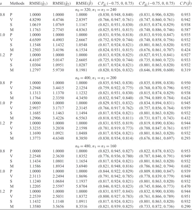
Table 1.Simulation results for the PLAM in the study
a Methods RMSE(gˆ1) RMSE(gˆ2) RMSE(β)ˆ C Pgˆ1(−0.75,0,0.75) C Pgˆ2(−0.75,0,0.75) C P(β)ˆ
n0=320,n1=n3=240
0.8 P 1.0000 1.0000 1.0000 (0.830,0.948,0.840) (0.831,0.906,0.820) 0.953 V 4.8290 4.4746 2.8397 (0.766,0.947,0.761) (0.747,0.860,0.761) 0.942 S 1.0619 1.0769 1.1167 (0.821,0.931,0.830) (0.815,0.874,0.829) 0.938 M 1.1763 2.7745 4.8363 (0.825,0.951,0.815) (0.748,0.886,0.746) 0.587 1.0 P 1.0000 1.0000 1.0000 (0.831,0.936,0.818) (0.813,0.910,0.847) 0.935 V 4.6509 4.4903 2.6667 (0.752,0.929,0.744) (0.748,0.858,0.756) 0.932 S 1.1548 1.1432 1.0548 (0.817,0.924,0.821) (0.801,0.863,0.820) 0.932 M 1.2503 3.4196 6.1534 (0.824,0.931,0.815) (0.676,0.861,0.707) 0.424 1.2 P 1.0000 1.0000 1.0000 (0.813,0.928,0.825) (0.827,0.913,0.841) 0.927 V 4.4107 5.0147 2.6605 (0.725,0.920,0.744) (0.735,0.860,0.723) 0.933 S 1.0304 1.0951 1.0287 (0.817,0.924,0.821) (0.801,0.863,0.820) 0.932 M 1.2797 5.9730 8.1981 (0.820,0.926,0.832) (0.646,0.898,0.608) 0.319
n0=400,n1=n3=200
0.8 P 1.0000 1.0000 1.0000 (0.835,0.943,0.838) (0.835,0.898,0.838) 0.950 V 3.2948 3.4415 2.1254 (0.759,0.922,0.775) (0.768,0.870,0.796) 0.952 S 1.1313 1.1370 1.1232 (0.821,0.931,0.830) (0.815,0.874,0.829) 0.938 M 1.1764 2.3350 4.3450 (0.832,0.947,0.840) (0.794,0.889,0.784) 0.624 1.0 P 1.0000 1.0000 1.0000 (0.829,0.921,0.832) (0.834,0.894,0.831) 0.945 V 2.9937 3.1717 2.3145 (0.766,0.917,0.762) (0.757,0.856,0.764) 0.939 S 1.1685 1.1463 1.1494 (0.817,0.924,0.821) (0.801,0.863,0.820) 0.932 M 1.2906 3.4226 6.5563 (0.818,0.923,0.811) (0.731,0.871,0.743) 0.432 1.2 P 1.0000 1.0000 1.0000 (0.831,0.935,0.819) (0.819,0.890,0.836) 0.944 V 3.3235 3.2038 2.1598 (0.781,0.919,0.773) (0.788,0.847,0.761) 0.937 S 1.1690 1.0921 1.0488 (0.817,0.924,0.821) (0.801,0.863,0.820) 0.932 M 1.3773 4.6348 8.3850 (0.830,0.934,0.814) (0.676,0.861,0.697) 0.293
n0=480,n1=n3=160
0.8 P 1.0000 1.0000 1.0000 (0.823,0.945,0.827) (0.822,0.878,0.832) 0.953 V 2.2548 2.3630 1.8352 (0.776,0.936,0.780) (0.787,0.846,0.791) 0.949 S 1.1434 1.0801 1.1654 (0.817,0.924,0.821) (0.801,0.863,0.820) 0.932 M 1.1586 1.8934 3.6940 (0.821,0.948,0.816) (0.786,0.862,0.794) 0.682 1.0 P 1.0000 1.0000 1.0000 (0.844,0.922,0.829) (0.809,0.880,0.847) 0.939 V 2.3113 2.2494 1.8696 (0.791,0.942,0.785) (0.778,0.839,0.779) 0.948 S 1.1240 1.0684 1.1937 (0.817,0.924,0.821) (0.801,0.863,0.820) 0.932 M 1.2205 2.5597 5.8704 (0.846,0.923,0.823) (0.745,0.866,0.773) 0.470 1.2 P 1.0000 1.0000 1.0000 (0.831,0.937,0.843) (0.832,0.900,0.830) 0.944 V 2.2539 2.5031 1.8372 (0.800,0.927,0.783) (0.761,0.866,0.789) 0.951 S 1.1432 1.1148 1.0911 (0.817,0.924,0.821) (0.801,0.863,0.820) 0.932 M 1.3580 3.5656 8.3516 (0.821,0.939,0.825) (0.733,0.872,0.736) 0.290
Notes: RMSE(gˆi), relative mean squared error forgˆi; RMSE(β)ˆ, relative MSE forβˆ;C P(β)ˆ, coverage probability of 95% nominal
CI forβˆ;C Pgˆi(−0.75,0,0.75), coverage probability of 95% nominal CI ofgˆi at−0.75, 0, 0.75,i=1,2; P, proposed estimator;
V, the estimator based on the SRS portion of the ODS design; S, the estimator based on an equal-sized SRS sample as the ODS design; M, the estimator treating ODS samples as SRS.
those at point−0.75 and 0.75, since more data are collected around point 0 and thus can fit better. With a larger sample, the coverage probabilities are expected to be improved. Note that the ODS design is a biased sampling design, so the M method which treats the ODS sample as if it was an SRS sample may result in inconsistent estimates. The obviously high RMSE(β)ˆ and low coverage probability ofβ using the M method exhibit evidence that ignoring the ODS design can result in biased estimation. However, unlike the case of a linear model or non-linear model with single monotonic non-linear function, in the ODS design of the CPP study which concentrates more resources on the tails of the outcome, we do not recognize an obvious pattern that the efficiency gain from the ODS design is higher with a low proportion of subjects in the SRS sample or with a high concentration of sampling at the tails of the outcome. This may be due to the introduction of more than one non-linear function simultaneously in the PLAM where these functions would possibly twist with each other. Therefore, how to obtain more informative supplemental samples and improve the efficiency of the ODS design for the case of additive models is an interesting topic and deserves further study in the future.
5. ANALYSIS OF THECPPDATA
As mentioned in the introduction section of the article, our motivating example is the CPP study where primary exposure (maternal pregnancy serum level of PCB) was found to have a non-linear relationship with the offspring’s subsequent IQ performance at age 7, so was another confounding variable EDU. We then apply our proposed PLAM accounting for both of the two possibly non-linear functions to the dataset, hoping to draw a more complete picture of the relation between prenatal PCB exposure and the children’s IQ scores.
In our analysis, we use the Weschler Intelligence Scale for children at 7 years of age (IQ), which had been observed for the entire CPP population, as the outcome variable and the prenatal PCB exposure level, measured through a serum assay with a relatively high cost, as the exposure variable. Additional confounding variables include the socioeconomic status of the children’s family (SES), the gender (SEX), and race (RACE) of the children, and their mother’s education (EDU).
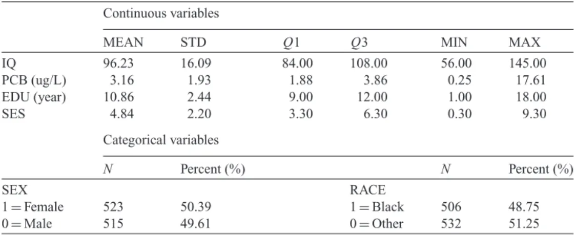
As only 1038 of the 1463 subjects obtained inGrayand others(2005) were observed to have complete data on all covariates, the ODS data structure for our CPP dataset becomes as follows: an overall SRS sample of 849 subjects, and two supplemental samples with 108 or 81 subjects from the children in the CPP population whose IQ scores are at least 1 standard deviation (14) above or below the mean (96), respectively. The description of the dataset is given in Table2. Note that we ignore any possible multicenter effect in the analysis presented here.
We then consider the following PLAM for the dataset:
IQ=β0+g1(PCB)+g2(EDU)+β1SES+β2RACE+β3SEX+, (5.1)
whereis a normal error with zero mean. Based on the previous partially linear studies, we adopt a 2-degree centered truncated power function with 10 fixed knots selected as the equally spaced sample quantiles of PCB level (1.16, 1.70, 2.17, 2.61, 3.05, 3.52, 4.06, 4.63, 5.54, and 6.88) to estimate the non-parametric functiong1(·)for PCB. And for estimation ofg2(·)for EDU, we adopt a 3-degree centered power spline with 5 fixed knots selected as the equally spaced sample quantiles of EDU (3, 6, 9, 12, and 15).
Table 2.Description of variables in the CPP analysis dataset(Ntotal=1038)
Continuous variables
MEAN STD Q1 Q3 MIN MAX
IQ 96.23 16.09 84.00 108.00 56.00 145.00
PCB (ug/L) 3.16 1.93 1.88 3.86 0.25 17.61
EDU (year) 10.86 2.44 9.00 12.00 1.00 18.00
SES 4.84 2.20 3.30 6.30 0.30 9.30
Categorical variables
N Percent (%) N Percent (%)
SEX RACE
1=Female 523 50.39 1=Black 506 48.75
0=Male 515 49.61 0=Other 532 51.25
Notes: For continuous variables: MEAN, mean of the variable; STD, standard deviation of the variable;Q1, 25% percentile of the variable;Q3, 75% percentile of the variable; MIN, minimum value of the variable; MAX, maximum value of the variable. For categorical variables:N: the number of subjects with the specific value of the variable; Percent:N/Ntotal.
Table 3.Estimates for the CPP analysis dataset
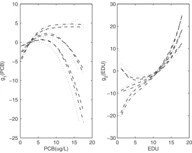
ˆ
βP SE(βˆP) 95%CI(βˆP) βˆV SE(βˆV) 95%CI(βˆV) βˆM SE(βˆM) 95%CI(βˆM) Intercept 95.27 1.32 (92.68, 97.86) 95.36 1.54 (92.34, 98.38) 95.62 1.59 (92.51, 98.73)
PCB See Figure 1 See Figure 1 See Figure 1
EDU See Figure 1 See Figure 1 See Figure 1
SES 1.04 0.22 (0.61,1.47) 0.97 0.26 (0.46,1.47) 1.25 0.26 (0.74,1.76)
RACE −8.28 0.76 (−9.77,−6.80) −7.90 0.90 (−9.67,−6.14) −10.14 0.92 (−11.94,−8.33) SEX −0.82 0.68 (−2.16,0.52) −0.76 0.84 (−2.40,0.87) −0.97 0.80 (−2.55,0.60)
Notes:βˆP,βˆV,andβˆMdenote the estimates obtained by the P, V, and M methods, respectively; SE(βˆP), SE(βˆV),and SE(βˆM)are the estimated standard errors of corresponding estimators; 95% CI(βˆP), 95% CI(βˆV),and 95% CI(βˆM)are the 95% CIs for the corresponding estimators.
From the left panel in Figure1, we can see that the IQ score is related to the PCB level non-linearly. The P estimator of the non-parametric functiong1shows that the relationship is positive in the lower range of PCB level, and then, after reaching a high point when the PCB level is about 7.44μg/L, a decreasing trend of the estimator is revealed. While most individuals only own a relatively low PCB level, this result should not be over-interpreted because of the possible existence of other uncaptured confounding variables like a higher fish intake during pregnancy mentioned inQin and Zhou(2011), which can both relate to a higher serum level of PCBs and a higher IQ in offspring.
The right panel in Figure1presents a similar story as withZhou, Youand others(2011) that there exists a clear non-linear positive relation between the mother’s education level (EDU) and child’s IQ score. The P estimate of the functiong2indicates that EDU has a much greater influence on children’s IQ around year 12 (i.e. after higher school education level), which completely agrees with previous results (Oddyand others,
2003;Breslauand others,2005).
Both panels in Figure1show that the P method yields smaller estimated variances and narrower 95% CIs than the V method.
0 5 10 15 20 −25
−20 −15 −10 −5 0 5 10
PCB(ug/L)
g1
(PCB)
0 5 10 15 20
−30 −20 −10 0 10 20 30
EDU
g 2
(EDU)
Fig. 1. The estimated function ofg1 on PCB (μg/L) andg2 on EDU. Thicker dashed curves, dotted curves and dot-dashed curves show the estimates and its corresponding estimated CIs obtained by the P, V, and M methods, respectively. P, proposed estimator; V, the estimator based on the SRS portion of the ODS design; M, the estimator treating ODS samples as SRS samples.
possibly due to the inconsistency of the M method. The conclusions by these three methods are consistent. The socioeconomic status of the child’s family is found to have a positive relation with the child’s IQ score, and blacks tend to have a worse IQ performance than children of other races. But no evidence has been shown that there exists an association between the child’s sex and IQ.
6. DISCUSSION
In this article, we innovatively introduced a PLAM for data obtained through an ODS design with a contin-uous outcome. To make inference under this biased sampling scheme, we proposed a penalized maximum likelihood method. Simulation studies shows that the proposed method yields more efficient estimates than those obtained from an SRS design with the same sample size across all the scenarios we considered, indicating that applying an ODS scheme in practice would actually reduce the study costs while achieving the same statistical efficiency by requiring a smaller sample size than the SRS design. This advantage is especially meaningful for a budget-limited study where measurement of the main exposure variable is really expensive, yet the outcome is relatively easy to obtain.
its two distributional tails, the observed exposure valuesXare also more likely to occur at its distributional tails. Therefore, we would expect an obvious efficiency gain from sampling at the tails of the outcome; the larger the proportion of sampling at tails, the more X values would occur at its distributional tails, and thus the more efficiency gain we would expect. However, this may not be the case when we allow for more than one non-linear, non-monotonic function in the model. Sampling more at the tails ofY does not necessarily indicate more covariates occurring at their tails. We are therefore not surprised when observing an unobvious efficiency gain when a larger proportion of sampling at tails is applied. Further studies are needed to explore how to obtain more informative supplemental samples of the ODS design under the framework of additive models.
SUPPLEMENTARY MATERIAL
Supplementary material is available athttp://biostatistics.oxfordjournals.org.
ACKNOWLEDGEMENTS
The authors thank the associate editor and two reviewers for constructive suggestions that largely improved the presentation of this article.Conflict of Interest:None declared.
FUNDING
G.Q. was supported by The National Natural Science Foundation of China (11371100) and H.Z. by National Institute of Health grants R01ES 021900 and P01CA142538.
REFERENCES
AERTS, M.,CLAESKENS, G.ANDWAND, M. P. (2002). Some theory for penalized spline generalized additive models.
Journal of Statistical Planning and Inference103, 455–470.
BRESLAU, N.,PANETH, N.ANDLUCIA, V. C. (2005). Paneth–Pollak R. Maternal smoking during pregnancy and
off-spring IQ.International Journal of Epidemiology34, 1047–1053.
CARROLL, R.,MAITY, A.,MAMMEN, E.ANDYU, K. (2009). Efficient semiparametric marginal estimation for the
partially linear additive model for longitudinal/clustered data.Statistics in Biosciences1, 10–31.
CHATTERJEE, N.,CHEN, Y. H.ANDBRESLOW, N. E. (2003). A pseudoscore estimator for regression problems with
two-phase sampling.Journal of the American Statistical Association98, 158–168.
CORNFIELD, J. (1951). A method of estimating comparative rates from clinical data; applications to cancer of the lung,
breast, and cervix.Journal of the National Cancer Institute11, 1269–1275.
COULL, J. T., NOBRE, A. C. AND FRITH, C. D. (2001). The noradrenergic alpha2 agonist clonidine modulates
behavioural and neuroanatomical correlates of human attentional orienting and alerting.Cerebral Cortex11, 73–84.
DING, J. L.,LIU, Y. Y.,PEDEN, D. B.,KLEEBERGER, S. R.ANDZHOU, H. B. (2012). Regression analysis for a summed missing data problem under an outcome-dependent sampling scheme.Canadian Journal of Statistics40, 282–303.
DING, J. L.,ZHOU, H. B.,LIU, Y. Y.,CAI, J. W.ANDLONGNECKER, M. P. (2014). Estimating effect of environmental contaminants on women’s subfecundity for the MoBa study data with an outcome-dependent sampling scheme.
GRAY, K. A.,KLEBANOFF, M. A.,BROCK, J. W.,ZHOU, H. B.,DARDEN, R.,NEEDHAM, L.ANDLONGNECKER, M. P. (2005). In utero exposure to background levels of polychlorinated biphenyls and cognitive functioning among school-age children.American Journal of Epidemiology162, 17–26.
HASTIE, T. (1996). Pseudosplines.Journal of the Royal Statistical Society Series B58, 379–396.
HASTIE, T.ANDTIBSHIRANI, R. (1990)Generalized Additive Models, 1st edition. London; New York: Chapman and
Hall.
HOLT, D.,SMITH, T. M. F.ANDWINTER, P. D. (1980). Regression-analysis of data from complex surveys.Journal of the Royal Statistical Society Series A143, 474–487.
HORVITZ, D. G.ANDTHOMPSON, D. J. (1952). A generalization of sampling without replacement from a finite universe.
Journal of the American Statistical Association47, 663–685.
LIANG, H.,THURSTON, S. W.,RUPPERT, D.,APANASOVICH, T.ANDHAUSER, R. (2008). Additive partial linear models
with measurement errors.Biometrika95, 667–678.
LINTON, O.ANDNIELSEN, J. P. (1995). A kernel-method of estimating structured nonparametric regression-based on
marginal integration.Biometrika82, 93–100.
LIU, L.,LI, J. B.ANDZHANG, R. Q. (2014). General partially linear additive transformation model with right-censored data.Journal of Applied Statistics41, 2257–2269.
LONGNECKER, M. P.,KLEBANOFF, M. A.,ZHOU, H. B.ANDBROCK, J. W. (2001). Association between maternal serum
concentration of the DDT metabolite DDE and preterm and small-for-gestational-age babies at birth.Lancet358, 110–114.
MARX, B. D.ANDEILERS, P. H. C. (1998). Direct generalized additive modeling with penalized likelihood. Computa-tional Statistics and Data Analysis28, 193–209.
NISWANDER, K. R.ANDGORDON, M. (1972). National institute of neurological diseases and stroke.The Women and
their Pregnancies; The Collaborative Perinatal Study of the National Institute of Neurological Diseases and Stroke. National Institute of Health; Washington: For sale by the Supt. of Docs., U.S. Govt. Print. Off.
ODDY, W. H.,KENDALL, G. E.,BLAIR, E.,DEKLERK, N. H.,STANLEY, F. J.,LANDAU, L. I.,SILBURN, S.ANDZUBRICK, S. (2003). Breast feeding and cognitive development in childhood: a prospective birth cohort study.Paediatric and Perinatal Epidemiology17, 81–90.
QIN, G. Y.ANDZHOU, H. B. (2011). Partial linear inference for a 2-stage outcome-dependent sampling design with a continuous outcome.Biostatistics12, 506–520.
QU, A. AND LI, R. (2006). Quadratic inference functions for varying coefficient models with longitudinal data.
Biometrics62, 379–391.
WEAVER, M. A.ANDZHOU, H. B. (2005). An estimated likelihood method for continuous outcome regression models
with outcome-dependent sampling.Journal of the American Statistical Association100, 459–469.
XU, W. L.ANDZHOU, H. B. (2012). Mixed effect regression analysis for a cluster-based two-stage outcome-auxiliary-dependent sampling design with a continuous outcome.Biostatistics13, 650–664.
YU, Y.ANDRUPPERT, D. (2002). Penalized spline estimation for partially linear single-index models.Journal of the
American Statistical Association97, 1042–1054.
ZHOU, H. B.,CHEN, J. W.,RISSANEN, T. H.,KORRICK, S. A.,HU, H.,SALONEN, J. T.ANDLONGNECKER, M. P. (2007). Outcome-dependent sampling: an efficient sampling and inference procedure for studies with a continuous out-come.Epidemiology18, 461–468.
ZHOU, H. B.,WEAVER, M. A.,QIN, J.,LONGNECKER, M. P.ANDWANG, M. C. (2002). A semiparametric empirical likelihood method for data from an outcome-dependent sampling scheme with a continuous outcome.Biometrics 58, 413–421.
ZHOU, H.,XU, W. L.,ZENG, D. L.ANDCAI, J. W. (2014). Semiparametric inference for data with a continuous outcome from a two-phase probability-dependent sampling scheme.Journal of the Royal Statistical Society Series B76, 197–215.
ZHOU, H. B.,YOU, J. H.,QIN, G. Y.ANDLONGNECKER, M. P. (2011). A partially linear regression model for data from an outcome-dependent sampling design.Journal of the Royal Statistical Society Series C60, 559–574.