i
PATTERNS OF BINGE DRINKING, MARIJUANA USE, AND DEPRESSIVE SYMPTOMS FROM ADOLESCENCE TO YOUNG ADULTHOOD: TESTING THE SELF-MEDICATION
AND STRESS MODELS
Andra Lea Wilkinson
A dissertation submitted to the faculty at the University of North Carolina at Chapel Hill in partial fulfillment of the requirements for the degree of Doctor of Philosophy in the Department of Maternal and Child Health in the Gillings School of Global Public Health.
Chapel Hill 2016
Approved by Carolyn T. Halpern Susan Ennett
Kathleen Mullan Harris Amy Herring
Jon Hussey
iii ABSTRACT
Andra Lea Wilkinson: Patterns of Binge Drinking, Marijuana Use, and Depressive Symptoms from Adolescence to Young Adulthood: Testing the Self-Medication and Stress Models
(Under the direction of Carolyn T. Halpern)
Understanding the relationships between substance use and depression could inform prevention and treatment efforts. Previous studies provide conflicting support for both depression leading to substance use—the Self-Medication Model—and substance use leading to
depression—the Stress Model. Much of this prior literature focuses only on adolescence,
examines only one direction, and/or fails to examine potential mediators or whether associations vary by biological sex.
Using data from Waves I, III, and IV of the National Longitudinal Study of Adolescent to Adult Health, mixed effects models were used to test the relationships between depressive symptoms and frequency of alcohol use and marijuana use across development, and whether these associations were moderated by sex. Regression models were used to examine potential mediators and one moderator for both the Self-Medication and Stress Models.
iv
norms also moderated this association for males. For females, the association between depressive symptoms and later marijuana use frequency may also be mediated by sensation seeking.
These results inform how to target and integrate screenings for adolescent substance use and depressive symptoms, both newly covered under the Affordable Care Act. For example, if adolescents screen positive for high or increasing depressive symptoms, it seems they should also be screened for marijuana use. Binge drinking screening could be targeted towards
adolescents with higher sensation seeking and depressive symptoms. The findings also indicate substance use and depression prevention and treatment programs should be integrated—as comorbidity is common—and tailored by sex—as the links between substance use and
v
To Darren Lee Legge,
vi
ACKNOWLEDGMENTS
This work would not have been possible without a large team of caring and brilliant people. My academic advisor in the Department of Maternal and Child Health and preceptor at the Carolina Population Center, Dr. Carolyn T. Halpern, has tirelessly mentored me on how I can be a better student, writer, scientist, teacher, and mentor for others. In addition to the lessons she imparts directly, she also leads by example. With the full workloads of at least four people, Dr. Halpern consistently provides thorough feedback on work you ask her to review, facilitates a safe learning environment for her students where we can learn from each other’s expertise and mistakes, and supports our scientific interests as they develop, even if they take us on paths diverging from her own. Not many advisors would work Thanksgiving Day to help you submit a training grant nor would they find and help you apply for a teaching innovation grant so you can develop a course in a new interest area nor would they support you spending a summer in South Africa exploring completely different research. Dr. Halpern has gone above and beyond as my teacher and mentor since before I was even her student and for this I am forever grateful.
vii
she knows it or not, to do more and do it better. I have also been lucky to take courses with and be mentored by Dr. Jon Hussey and Dr. Susan Ennett, both of whom have incredibly incisive minds that have challenged me—over and over again—to maximize the lucidity and depth of my research methods. Thank you both for repeatedly making me think so hard my head hurt! Next, I idolized Dr. Kathleen Mullan Harris for years before I met her, for her leadership of the National Longitudinal Study of Adolescent to Adult Health, among other things. With seemingly
impossible demands on her time, Dr. Harris has enthusiastically engaged with me on several papers, providing invaluable feedback from a sociological lens, which has only strengthened my work. Last but certainly not least, Dr. Meghan Shanahan, having little knowledge of my work or the subject area, cheerfully joined the Committee and charitably spent countless hours reading the papers in detail and asking the insightful questions that pushed me to maximize the clarity of my work.
In addition to being surrounded by incredible mentors, I have also been in hugely supportive environments that have accelerated my learning above and beyond typical graduate training. First, the Maternal and Child Health Department was my first home away from home; thank you for charming me with and maintaining your wonderful balance of being a national and international leader in the field that still hosts homey and welcoming potlucks. Thank you for nominating me for numerous opportunities, including the Student Leadership Institute of the Association of Schools and Programs in Public Health. Thank you to the faculty in the
Department for repeatedly investing in your classes and students, patiently answering my endless list of questions, and inviting me to lecture in your classrooms; these were experiences I
viii
thank you for your listening ear, thoughtful advice, and incredible snacks. Dr. Anita Farel, thank you for being my ally from day one through good and trying times; I do not want to imagine what this journey would have been like without having you in my corner.
Second, the Gillings School of Global Public Health provided a collaborative and innovative playground that has been so much fun to learn in! Thank you to the faculty in the School for teaching wonderful courses and inviting me onto projects that greatly expanded my horizons, namely Dr. Audrey Pettifor in Epidemiology, Dr. Wizdom Powell Hammond in Health Behavior, and Dr. Stephanie Wheeler and Dr. Kristen Hassmiller Lich in Health Policy and Management. It was wonderfully enriching to receive such interdisciplinary training.
Third, I view being a trainee at the Carolina Population Center over the last four years as one of the great fortunes of my graduate training. The Center has provided training support (T32-HD007168) and general support (R24-HD050924) and so much more. Thank you to Jan
Hendrickson-Smith for always pushing herself and the trainees for excellence. Jan helped me apply for the traineeship before I was even on campus, encouraged me to meet with visiting speakers before I felt qualified to do so, and convinced me applying for a training grant through the National Institutes of Health in my first semester of graduate school was not ludicrous. Indeed it was only with the support of CPC, namely Pandora Riggs, Deb Ussery, Tom Swasey, Dr. Eric Whitsel, Dr. Amy Herring, and of course Dr. Carolyn T. Halpern that the application was possible and ultimately successful (F31-DA036961). Further, it was only with the dedicated CPC team that I have been able to carry out the work. Thank you to Dr. Mariah Cheng, Ping Chen, Phil Bardsley, Denise Ammons, Jamie Shea, Joyce Tabor, Tim Van Acker, Lori Delaney, and Tom Heath for making it all run smoothly! I am also grateful to the researchers and
ix
program project directed by Kathleen Mullan Harris and designed by J. Richard Udry, Peter S. Bearman, and Kathleen Mullan Harris at the University of North Carolina at Chapel Hill, and funded by grant P01-HD31921 from the Eunice Kennedy Shriver National Institute of Child Health and Human Development, with cooperative funding from 23 other federal agencies and foundations. No direct support was received from grant P01-HD31921 for this analysis. All Add Health procedures were approved by the Public Health Institutional Review Board (IRB) at the University of North Carolina at Chapel Hill; the present dissertation analyses were deemed exempt.
x
TABLE OF CONTENTS
LIST OF TABLES ... xii
LIST OF FIGURES ... xiv
LIST OF ABBREVIATIONS ... xv
CHAPTER 1 - INTRODUCTION ... 1
Specific Aims ... 1
Background & Significance ... 2
Limitations of Past Literature ... 9
Conceptual basis ... 10
Aim 1 Methods ... 16
Aim 2 Methods ... 26
Sample & Power... 37
CHAPTER 2 – TESTING RELATIONSHIPS BETWEEN BINGE DRINKING, MARIJUANA USE, AND DEPRESSIVE SYMPTOMS AND MODERATION BY BIOLOGICAL SEX... 43
Overview ... 43
Introduction ... 44
Methods ... 47
Results ... 49
Discussion ... 56
xi
Overview ... 61
Introduction ... 62
Methods ... 65
Results ... 69
Discussion ... 73
CHAPTER 4– CONCLUSIONS & IMPLICATIONS FOR CARE ... 78
Conclusions ... 78
Innovation... 80
Limitations ... 82
Implications for Health... 84
APPENDIX 2.1: ANALYSES ... 90
APPENDIX 2.2: BINGE DRINKING FREQUENCY GROWTH CURVES ... 92
APPENDIX 2.3: MARIJUANA USE FREQUENCY GROWTH CURVES ... 97
APPENDIX 2.4: DEPRESSIVE SYMPTOM GROWTH CURVES ... 101
APPENDIX 3.1: HYPOTHESES ... 109
APPENDIX 3.2: ANALYSES ... 112
APPENDIX 3.3: SENSATION SEEKING MEDIATION FOR SELF-MEDICATION MODEL ... 113
APPENDIX 3.4: AGB MEDIATION FOR SELF-MEDICATION MODEL... 118
APPENDIX 3.5: CRP AND EBV MEDIATION FOR STRESS MODEL ... 122
APPENDIX 3.6: AGB MEDIATION FOR STRESS MODEL ... 134
APPENDIX 3.7: AGB MODERATION OF THE SELF-MEDICATION MODEL ... 138
xii
LIST OF TABLES
Table 1.1: Depressive symptom items for the CES-D (Waves I, III, and IV) ... 17
Table 1.2: Cronbach’s alpha for the CES-D for males and females (Waves I, III, and IV) ... 18
Table 1.3: Binge drinking items (Waves I, III and IV) ... 19
Table 1.4: Marijuana use items (Waves I, III, and IV) ... 20
Table 1.5: Measure transformations for marijuana use ... 20
Table 1.6: Sensation seeking items (Wave III) ... 32
Table 1.7: Characteristics of the analysis sample ... 38
Table 2.1: Characteristics of the analysis sample by age... 51
Table 3.1: Characteristics of the mediation analysis sample ... 70
Table 2.2.1: Linear mixed effects models of binge drinking frequency with depressive symptoms tested as a predictor ... 94
Table 2.3.1: Linear mixed effects models of marijuana use frequency with depressive symptoms tested as a predictor ... 98
Table 2.4.1: Linear mixed effects models of depressive symptoms ... 102
Table 2.4.2: Linear mixed effects models of depressive symptoms with binge drinking frequency tested as a predictor ... 104
Table 2.4.3: Linear mixed effects models of depressive symptoms with marijuana frequency tested as a predictor ... 106
Table 3.3.1: Linear regression testing mediation of the Self-Medication Model by sensation seeking, Males ... 113
Table 3.3.2: Linear regression testing mediation of the Self-Medication Model by sensation seeking, Females ... 115
Table 3.4.1: Linear regression testing mediation of the Self-Medication Model by AGB, Males ... 118
xiii
Table 3.5.1: Regression testing mediation of the Stress Model by high sensitivity C-reactive protein, Males ... 122 Table 3.5.2: Regression testing mediation of the Stress Model by high sensitivity
C-reactive protein, Females ... 125 Table 3.5.3: Linear regression testing mediation of the Stress Model by Epstein-Barr
Virus, Males ... 128 Table 3.5.4: Linear regression testing mediation of the Stress Model by Epstein-Barr
Virus, Females ... 130 Table 3.6.1: Linear regression testing mediation of the Stress Model by Adherence to
Gender-typical Behavior, Males ... 134 Table 3.6.2: Linear regression testing mediation of the Stress Model by Adherence to
Gender-typical Behavior, Females ... 136 Table 3.7.1: Linear regression testing moderation of the Self-Medication Model for binge
xiv
LIST OF FIGURES
Figure 1.1: Conceptual models for the Self-Medication and Stress Models ... 11 Figure 1.2: Distribution of males and females by predicted probability of being male
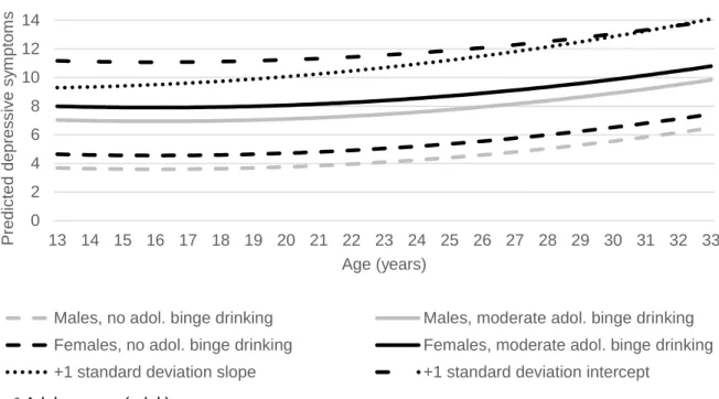
(Wave I) ... 29 Figure 1.3: Mediation analysis framework ... 35 Figure 2.1: Key coefficients from the linear mixed effects models ... 54 Figure 2.2: Relationship between adolescent depressive symptoms and marijuana use
frequency growth curve (Self-Medication Model) ... 55 Figure 2.3: Relationship between adolescent binge drinking frequency and depressive
symptoms growth curve (Stress Model) ... 56 Figure 3.1: Distribution of males and females by predicted probability of being male
(Wave III)... 68 Figure 3.2: Significant coefficients from the regression models testing mediation ... 72 Figure 3.3: AGB moderation of the association between depressive symptoms and later
xv
LIST OF ABBREVIATIONS AAP American Academy of Pediatrics
ACA Affordable Care Act
Add Health National Longitudinal Study of Adolescent to Adult Health
AGB Adherence to Gender-typical Behavior BIC Bayesian Information Criterion
CMS Centers for Medicare and Medicaid Services
CES-D Center for Epidemiologic Studies Depression Scale CRP High sensitivity C-reactive protein
EBV Epstein-Barr virus
ICC Intraclass Correlation Coefficient
SBIRT Screening, brief interventions, and referral to treatment
SD Standard deviation
1
1
CHAPTER 1 - INTRODUCTION
Specific Aims
Adolescence is characterized by increasing substance use and depressive symptoms, both of which can have short- and long-term implications.1–4 Many studies have found strong
correlations between substance use and depression, though it is not clear if the association is causal, and if it is, in which direction(s) the process operates. Some studies find that depression leads to substance use, possibly by lowering the accuracy of risk perceptions and decreasing impulse control; we label this pathway the Self-Medication Model.4–6 Other studies suggest substance use leads to depression.5,7,8 We label this pathway the Stress Model, as a hypothesized mechanism underlying it involves the stress response, the body’s endocrine reaction to novelty exposure, which can be stimulated by risk taking and, when chronic, can lead to depression.9–13 Complicating potential causal pathways, there are biological sex (sex) differences in the
prevalence of substance use and depression, as well as differences in responsiveness to stress.4,14–
16 Findings to date suggest the Self-Medication Model may be more relevant for males, whereas
females might be better represented by the Stress Model.10,11,16–18
2
Health (Add Health), which includes a representative sample of more than 20,000 adolescents in grades 7-12 in the 1994-95 school year who have been followed prospectively for 15 years as they transitioned to young adulthood. Present analyses addressed the following two study aims: Aim 1. Evaluate empirical support for the Self-Medication and Stress Models by estimating growth curves of alcohol use, marijuana use, and depressive symptoms and testing whether these trajectories are conditioned by biological sex and/or are related to each other.
Aim 2. Using regression models, examine potential mediators (sensation seeking, stress biomarkers, and gender norm adherence) and a moderator (gender norm adherence) of the relationships between substance use and depressive symptoms and whether the relationships differ by biological sex.
Background & Significance
During adolescence, sensation seeking increases while impulse control is still developing; this creates a developmental window where adolescents often experiment with facets of adult behavior, like substance use.4,24 Risk taking can also facilitate peer group bonding, which is a critical aspect of development as adolescents distance themselves from parents and family.3
However, too much risk taking, and certain types of risk taking, can be harmful. Most substance use is initiated in adolescence, a developmental period often recognized as lasting from age 12 to 19.4,15 The trajectory typically begins with alcohol and tobacco use before or early in high
school, then may escalate to use of illicit drugs (e.g., heroin) during high school.4 According to the 2013 Youth Risk Behavior Survey, more than one-third of high school students report current alcohol use, and smoking marijuana (23.4%) is now more common than smoking cigarettes (15.7%) among adolescents.25 Alcohol and marijuana are the two most commonly used
3
significant psychological changes.4,25 Therefore alcohol and marijuana use are the focus of this research project.
The quantity and frequency of alcohol and drug use typically peak between 18-25 years of age in the United States.4 On average, adolescent males use more substances and use them more frequently than females, though this can vary by age, with females engaging in more substance use than males in early adolescence.4,25,26 By middle to late adolescence, males are more likely to engage in regular substance use. By comparison, females may accelerate faster than males from initiating use to experiencing problems from use.4,27 Substance use in
adolescence can have significant health effects (e.g., substance dependency or abuse, adverse effects on brain development) as well as deleterious effects on a wide range of developmental outcomes (e.g., educational attainment).4
Depression is also prevalent in adolescence. The International Classification of Diseases characterizes depression as including some or all of the following symptoms: a depressed mood, loss of interest and enjoyment, reduced activity, disturbed sleep and appetite, decreased self-esteem, and/or guilt. Diagnoses of mild, moderate, or severe depression depend on the number of symptoms a person experiences and the degree to which a person can continue with their daily activities.28 A systematic review conducted for the United States Preventive Services Task Force
(USPSTF) estimates that the prevalence of current or recent depression in adolescence is 6% and the lifetime prevalence of major depressive disorders among adolescents is as high as 20%.2 In adolescence and beyond, females are more likely to experience depression than males.14 Early onset depression (before age 21) is associated with an increased risk of suicide attempts, death by suicide, longer episodes of depression and higher rates of recurrence.2,29 Adolescent depression
4
relationships) and the long-term (e.g., decreased educational attainment).1,2,29 At a population level, depression is one of the most burdensome diseases globally because of its early age of onset, tendency to be chronic, impairment of normal activities, and high lifetime prevalence.22
Depression and substance use are often comorbid.23,30 For example, results from the 2013 National Survey on Drug Use and Health revealed 11.8% of 12-17 year-olds without a major depressive episode in the past year reported marijuana use in the past year compared to 25.7% of adolescents who did have a major depressive episode in the past year.31 Comorbidity of
substance use and depression in adolescence is associated with multiple negative outcomes including more severe mental health issues, increases in substance use, delays in substance abuse recovery, longer depressive episodes, and elevated suicide risk.21 The comorbidity between
substance use and depression could indicate several possible relationships between the two. Fleming et al. outlined four possible forms of relationships underlying the comorbidity.32 First, it is possible the levels of depression and substance use are concurrently associated across time. Second, change in one may be associated with change in the other across development. Third, it is possible the two conditions are only related at specific time points during development. Finally, the relationship may be predictive, meaning one generally precedes and predicts the other; both the Self-Medication and Stress Models are examples of predictive relationships.32
Understanding the relationship between substance use and depressive symptoms during development is important because it could inform screening, prevention, and treatment practices. Surveys of physicians indicate approximately less than half screen their patients for substance use or depression, and it is likely even rarer for adolescent patients.33,34 As a consequence, most cases of substance use problems and depression in adolescence go untreated.2,33,35 This is a
5
estimated 50% of mental health and substance use conditions begin by age 14.2,35–37 Though the Affordable Care Act (ACA) now ensures insurance companies will cover screening, it does not mandate that physicians provide the screening.38 Surveys of physicians indicate they feel time constrained and uncomfortable treating or providing referrals for substance use or depression issues.2,39 Therefore, understanding, for example, that depression generally precedes substance use issues, especially in males, helps physicians target screening and integrate treatment and referral steps accordingly.
Self-Medication Model
The Self-Medication Model, first articulated in the 1990s by Harvard Psychiatrist Dr. Edward Khantzian, holds that people struggling with depression may engage in substance use in an attempt to ameliorate their symptoms.40–42 This pathway is facilitated by the process of depression impairing cognitive function and memory, decreasing impulse control, and impairing psychosocial functioning, (e.g., motivation), all of which can impair accurate risk perceptions.4,42 Adolescents may be especially vulnerable to these processes because of existing imbalances between impulsivity and reasoned decisions, and their lesser experience with self-regulation.24
Evidence for this model includes the finding that adolescents taking antidepressants experience consequent declines in substance use.43 Expanding beyond depression to internalizing symptoms
in general (e.g., anxiety), many studies have connected internalizing symptoms/problems in childhood to substance use in adolescence and young adulthood.44 Further, studies have found reports of self-medication as a primary reason for addiction among certain populations.42,44 Stress Model
6
stress and chronic stress can harm the body; one possible harm is increased depressive
symptoms.45 If the brain perceives risk taking such as substance use as a threat, it stimulates both
the sympathetic-adrenal-medullary axis and the hypothalamic-pituitary axis, leading to, among other things, cortisol release.9,45 Chronically elevated cortisol levels can lead to dysregulated affect, possibly by changing the functional connectivity of the amygdala-ventromedial prefrontal cortex, which is positively associated with depression.12,13 The stress response also increases inflammation.46,47 Inflammation can contribute to depression through effects on neurotransmitter
metabolism, neuroendocrine function, synaptic plasticity, and information processing.48,49 Past studies have tested whether substance use is associated with later increases in depressive symptoms, but few have articulated conceptual grounding for it.5–8
Past Literature
Many prior studies have attempted to tease apart the comorbidity between depression or depressive symptoms and substance use. The bulk of this research has been motivated by the Self-Medication Model, and several longitudinal studies have found support for this
model.6,21,22,42 For example, Burns et al. followed a sample of 64 rural adolescents from ages 12 to 18 and found baseline depression was significantly associated with substance abuse at follow-up, controlling for sex.50 Henry et al. analyzed a birth cohort of over 700 males and females in
7
found depression actually decreased the odds of substance use among females abstaining from substances at Wave I.5
More recent studies have used methods that allow analysis of individual trajectories (e.g., growth curve and latent growth curve analysis, hierarchical linear modeling, growth mixture modeling). Repetto, Zimmerman, and Caldwell used hierarchical linear models with data from over 600 African American youth surveyed annually for six years to estimate the growth curves of marijuana use and depression and test their inter-relationships as well as potential moderators. One finding, among others, was that higher depressive symptoms predicted increases in later marijuana use, but only for males. For females, those with lower depressive symptoms used more marijuana than those with higher depressive symptoms, somewhat matching the results from Hallfors et al.5,21 Hooshmand, Willoughby, and Good used latent growth curve models to analyze data from over 4,000 Canadian high school students and found that adolescents with higher depressive symptoms in grade 9 had faster increases in marijuana use frequency during high school, but not the other way around and not for alcohol use.6
8
for the Stress Model.7 Fergusson et al., with a sample of over 1,000 late adolescents followed into emerging adulthood, tested both potential directions of the association between alcohol abuse or dependence and depression, and found the best fitting model supported a pathway leading from alcohol problems to depression.51 Three recent reviews found evidence of alcohol or marijuana use being associated with later depression.52–54
At least two studies have had more nuanced results. First, Needham used data from Add Health Waves I, II, and III to test sex-stratified latent growth curve models of both directions of the association.22 Adolescent males and females with higher depressive symptoms at Wave I had higher levels of binge drinking at Wave I but the smallest odds of further increases in binge drinking compared to those with lower depressive symptoms at Wave I. Similarly, adolescent females with higher depressive symptoms at Wave I had higher levels of illicit substance use at Waves I, II, and III though smaller odds of further increases in illicit substance use compared to females with lower depressive symptoms at Wave I. The author interpreted these results as support for the Self-Medication Model, even though she did not find support for an expected accumulation in disadvantage (i.e., increases in substance use over time). Findings for the Stress model followed a similar pattern; adolescents with higher binge drinking or substance use at Wave I had consistently higher depressive symptoms, though they declined at a faster rate, than their peers who were not using any substances at Wave I. The author interpreted the results overall as support for a bi-directional relationship between substance use and depression, though the results could also be interpreted as a concurrent relationship in adolescence that faded with development.22 Similarly, Costello et al. used latent trajectory analysis to model trajectories of depressive symptoms using Waves I, II, and III of Add Health.8 They found adolescents who
9
show a depressive symptom trajectory characterized by high levels at Wave I that declined over time.8,22 However, despite the decline, substance using adolescents had consistently higher levels
of depressive symptoms compared to adolescents who did not use substances.
Interestingly, another study used longitudinal mixed effects models with Add Health data and found support for a bidirectional relationship.55 In support of the Self-Medication Model, a five-point increase in depressive symptoms at an earlier wave was significantly associated with approximately a half-day increase in cigarette smoking frequency at a later wave, but only for females. In support of the Stress Model, a 5-day increase in cigarette smoking frequency in the past month at an earlier wave was associated with a 0.02-point increase for males and a 0.05-point increase for females in depressive symptoms at a later wave. Marijuana use and binge drinking were also tested but no significant associations were found.
Finally, at least one analysis has had null findings. Fleming et al. used multivariate latent trajectory modeling with data from over 1,000 males and females surveyed annually from 8th to 11th grade in the Pacific Northwest of the United States to test cross-sectional, concurrent over time (longitudinal), and predictive (e.g., earlier measure predicting a later change) relationships between depressive symptoms and substance use. While they found significant concurrent relationships, perplexingly, they found no significant predictive relationships that supported either Model. However, they did find that higher levels of depressive symptoms predicted a slower increase in alcohol use compared to lower levels of depressive symptoms, which is a challenge to the Self-Medication Model.32
Limitations of Past Literature
10
of the relationship between adolescent substance use and depression, they still share many limitations. Prior trajectory analyses in this topic area have disproportionately examined the Self-Medication Model, failing to test the Stress Model. Further, many studies seem restricted to small, non-representative samples (e.g., school- or clinic-based samples) that are followed only during adolescence (e.g., 9th through 12th grade). Also, the studies have been focused on the temporal relationship between substance use and depressive symptoms and therefore have left other relevant research questions like moderation by sex and potential mediators largely untested. In fact, two reviews of this literature have called for more studies examining differences by biological sex.53,54 The aims of this study address each of these limitations.
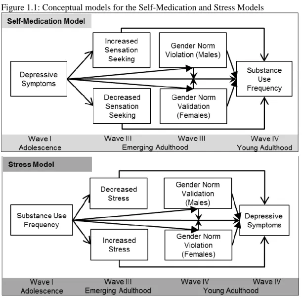
Conceptual basis
11
Figure 1.1: Conceptual models for the Self-Medication and Stress Models
Self-Medication Model
The top of the figure illustrates the Self-Medication Model. As previously described, the Self-Medication Model holds that adolescents struggling with depression may engage in
12
illusion of relieving depressive symptoms such as isolation and emptiness.42 As such, alcohol use for adolescents could be used to feel relief from social isolation amid new peer groups, for example, and gain a sense of belonging from engaging in a normative activity.6
An important potential mediator for the Self-Medication Model is sensation seeking. Sensation seeking has been found to predict alcohol and substance use in adolescents.58
Sensation seeking has also been implicated in the relationship between depressive symptoms and substance use. Researchers with data from over 4,000 Canadian adolescents who were surveyed each year of high school used latent class growth analysis to determine that adolescents who scored high in sensation seeking were at a higher risk of being in the trajectory of co-occurring depressive symptoms and alcohol use compared to singular trajectories of either one. Further, adolescents who scored low in novelty seeking were much less likely to be in the alcohol use trajectory.59 Pahl, Brook, and Koppel controlled for sensation seeking when assessing the
relationship between marijuana use and depressive symptoms and the relationship persisted, indicating sensation seeking was not confounding the association as a shared predictor.7 Given this, it seems reasonable to test whether it is a mediator. Adherence to gender norms will be discussed as a potential mediator and/or moderator in a later section.
Stress Model
sympathetic-13
adrenal-medullary axis and the hypothalamic-pituitary axis, which then activates the release of catecholamines and glucocorticoids to ready the body for fight or flight.45 These responses are
acutely adaptive but when repeatedly stimulated can cause the downstream systems to first overcompensate and then dysregulate.45 In the brain, this can result in remodeling of dendrites and synapses, suppression of new cell growth, and changes in neurotransmitter metabolism and overall neuroendocrine functioning; all of which are implicated in depression.45,48,49 For
example, changes in the metabolisms of serotonin, dopamine, or norepinephrine—the neurotransmitters targeted by depression medications—would likely induce depression.48 Further, hypersecretion of corticotrophin-releasing hormone—a key regulator of hormonal responses to stress—is often found in patients with depression.48
Biological Sex and Gender Differences in Self-Medication and Stress Models
14
emotional coping mechanisms and so females, even if they experience depression in similar ways to males, may still have less incentive to use substances in an attempt to self-medicate.17
By comparison, we have reason to expect depressive symptoms to have a stronger relationship with sensation seeking and substance use for males. First, compared to females, males are less likely to emotionally regulate and more likely to practice impulsive or reward-seeking behavior, especially drinking alcohol.17,61,62 Males experiencing depressive symptoms may have or perceive they have no means of regulating or coping with their emotions beyond sensation seeking. In fact, among a sample of social drinkers, males were more likely than females to report drinking in order to regulate negative affect.63 Second, where depressive symptoms are considered socially acceptable for females, for males they can be perceived as a violation of masculine gender norms like invulnerability.64 A male experiencing depressive symptoms may feel he is weak or vulnerable due to a perceived lack of emotion regulation tools and/or the perceived violation of masculine norms. From this place of vulnerability, substance use may be an easily accessible means of engaging in risk taking, a key way to demonstrate adherence to masculine gender norms for young men.22,65
For the Stress Model, evidence suggests females may be more likely to experience stress and subsequent depression from substance use. Female gender norms can emphasize risk
aversion and, to the degree these norms are enforced, this can in turn influence how much stress females may experience from substance use.18 For example, parental regulation is usually stronger or lasts longer for female children, and so they may come to perceive more negative consequences from risk taking that defies gender norms, and thus may have a stronger stress response to substance use.10,66 Additionally, females are thought to have both greater sensitivity
15
females experienced interpersonal stressors from substance use (e.g., parental or peer disapproval), females may be more likely to perceive the stress and react negatively to it. If substance use increases interpersonal stress with peers, parents, and/or teachers, this process might account for females’ greater vulnerability to depressive symptoms.3,18,67 Finally, females may be more vulnerable to inflammation, strengthening the relationship between stress and depressive symptoms for them compared to males. During adolescence, females develop higher, on average, baseline levels of inflammation compared to males. A cross-sectional analysis of age cohorts spanning from childhood to young adulthood using the National Health and Nutrition Examination Survey found that between ages 16 and 19 a gap emerges in inflammation levels between males and females, with the latter being significantly higher. It is important to note this gap emerges at an unusual time point as it does not coincide with the onset of puberty and thus may be due to behavioral or social, rather than biological, differences in males and females.68
Therefore, even if risk taking elicits a similar stress response in males and females, with higher baseline inflammation levels, females could still be more vulnerable to a depressive response.47,68
In contrast, for males, there are both social and biological reasons to expect less support for the Stress Model. In general, risk taking is much more common among adolescent males compared to adolescent females. For example, young men are less likely to wear bike helmets, more likely to drive recklessly, have more sexual partners on average, and are less likely to seek health care compared to young women.64,65 This sex disparity in risk taking behavior could be due to the fact that men, on average, perceive less risk than women do when confronted with the same situation.69 Alternatively, risk taking is a key way for young men to demonstrate
16
levels of substance use.71–74 In addition to this social explanation for adolescent males’ apparent affinity for risk taking, there is a potential biological explanation. Cortisol, the main hormone of the stress response, is inhibited by testosterone, which is at higher levels in males than females. In fact, one study of 150 young adult males found their cortisol responsiveness to stress varied and those with weaker responses were more likely to engage in high-risk sexual behaviors.3 Given the prevalence of risk taking behaviors, including substance use, among males and the potential social explanations, it seems reasonable to expect a null or even negative relationship between substance use, stress, and subsequent depressive symptoms for males.6,42,57,62 Overall, biological sex and/or gender differences could influence the direct associations between depressive symptoms and substance use as well as potential mediation paths in both the Self-Medication and Stress Models.
Aim 1 Methods
Aim 1. Evaluate empirical support for the Self-Medication and Stress Models by estimating growth curves of alcohol use, marijuana use, and depressive symptoms and testing whether these trajectories are conditioned by biological sex and/or are related to each other. Study Sample
17
interview data are excluded from these analyses because it was just one year later and by design did not include the Wave I seniors. Wave III interviews (n=15,197) were completed in 2001-02, when respondents were ages 18-26. Response rates exceeded 75% at all waves. Wave IV interviews occurred in 2008-09 when respondents were ages 24-32. An 80% re-interview rate was achievedfor Wave IV, yielding information for 15,701original Add Health respondents. Aim 1 Measures
Depressive Symptoms: Depressive symptoms were measured using the Center for Epidemiologic Studies Depression Scale (CES-D), first created in 1977 it remains a common scale for depression epidemiology.76 The items in the scale are designed to capture the frequency of types of depression symptoms (e.g., symptoms related to sadness, appetite, being tired, etc.) outlined in the American Psychiatric Association Diagnostic and Statistical Manual, though it is not a diagnostic tool.76 Nine items from the CES-D were included in the Wave I, III, and IV
surveys. Summed scores range from 0-27; higher scores indicate more and/or more frequent symptoms. The CES-D captures depressive symptoms within the past week (e.g., felt sad, tired all the time) (Table 1.1), though 12-month re-test reliability ranges from 0.4-0.7.76 Adjusting the CES-D scores for participants using antidepressants was not possible, as measures of
antidepressant use were only collected at Wave IV, and thus similar adjustments could not be made at all waves of data used in the analysis.
Table 1.1: Depressive symptom items for the CES-D (Waves I, III, and IV)
Item Wording Item Response
How often was the following true during the past week?
You felt sad 0: Never or rarely
You felt you were just as good as other people 1: Sometimes You felt that people disliked you 2: A lot of the time
You felt depressed 3: Most/all of the time
You felt you were too tired to do things 6: Refused
18 You were bothered by things that usually don’t
bother you
You had trouble keeping your mind on what you were doing
You felt that you could not shake off the blues, even with help from your family and your friends
Table 1.2 below shows the reliability estimates for the CES-D in this sample, or their coherence in measuring the same thing. The Cronbach’s alpha value estimates the proportion of each item’s variation that is shared with variation in the latent construct of depressive symptoms. Table 1.2: Cronbach’s alpha for the CES-D for males and females (Waves I, III, and IV)
Wave I CES-D 0.79 Wave III CES-D 0.80 Wave IV CES-D 0.81
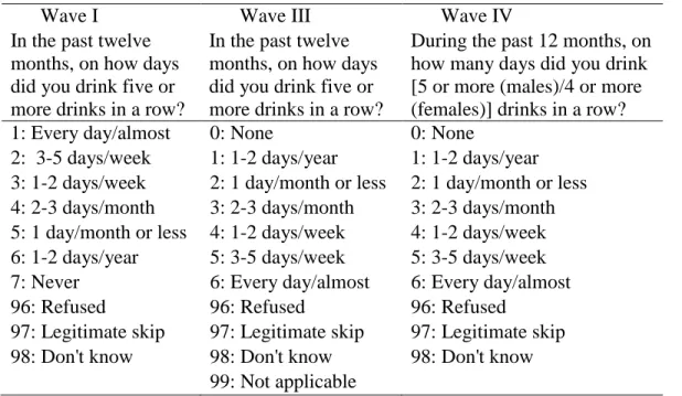
Substance Use: For substance use, we focused on the two most commonly used substances (alcohol and marijuana), both of which have in-depth measurement at each wave (Tables 1.3 and 1.4).25 For marijuana use, at Waves I and III, respondents were asked how many times they used in the past thirty days (e.g., 0 to >900). At Wave IV, the question changed to measure on how many days respondents used marijuana in the past thirty using a 0 to 6 ordinal scale for none to nearly every day. To make the measures of marijuana use frequency
comparable at each wave, we derived the number of days of use in a given time period from the times of use reported in Waves I and III (Table 1.5). This derived measure assumes that someone reporting four times of use in the past month at Wave I used about once per week rather than four times in one day, but for this research we care more about the frequency of use and less about the distribution of use.
For alcohol use, as it is a much more commonly reported behavior among adolescents than marijuana, we used a measure of binge drinking frequency to try to capture more
19
was assessed for the past year using the same ordinal variable of 0 for none to 6 for nearly every day. At Waves I and III, binge drinking was defined as drinking five or more drinks in a row, but at Wave IV the measure was specified as four or more drinks for women and five or more drinks for men to match the definition of binge drinking from the Centers for Disease Control and Prevention.77,78 Originally, the measures for both binge drinking and marijuana use were derived as the midpoint from the range of number of days of use, but these measures had too much weight in the tail, so we moved to a rank category measure for marijuana use and kept the ordinal measure for binge drinking frequency. The Bayesian Information Criterion (BIC) model fit index was used to compare the models using the midpoint frequency and rank category measures and they were very similar.
Table 1.3: Binge drinking items (Waves I, III and IV)
Wave I Wave III Wave IV
In the past twelve months, on how days did you drink five or more drinks in a row?
In the past twelve months, on how days did you drink five or more drinks in a row?
During the past 12 months, on how many days did you drink [5 or more (males)/4 or more (females)] drinks in a row? 1: Every day/almost 0: None 0: None
2: 3-5 days/week 1: 1-2 days/year 1: 1-2 days/year 3: 1-2 days/week 2: 1 day/month or less 2: 1 day/month or less 4: 2-3 days/month 3: 2-3 days/month 3: 2-3 days/month 5: 1 day/month or less 4: 1-2 days/week 4: 1-2 days/week 6: 1-2 days/year 5: 3-5 days/week 5: 3-5 days/week 7: Never 6: Every day/almost 6: Every day/almost
96: Refused 96: Refused 96: Refused
97: Legitimate skip 97: Legitimate skip 97: Legitimate skip 98: Don't know 98: Don't know 98: Don't know
20 Table 1.4: Marijuana use items (Waves I, III, and IV)
Wave I
Wave III Wave IV
During the past 30 days, how many times have you used marijuana?
During the past 30 days, how many times have you used marijuana?
During the past 30 days, on how many days did you use marijuana? 0: Minimum value 0: Minimum value 0: None
900: Maximum value 999: Maximum value 1: 1 day
996: Refused 9996: Refused 2: 2-3 days
997: Legitimate skip 9997: Legitimate skip 3: 1 day/week 998: Don't know 9998: Don't know 4: 2 days/week 999: Not applicable 9999: Not applicable 5: 3-5 days/week
6: Every day/almost 96: Refused
97: Legitimate skip 98: Don't know Table 1.5: Measure transformations for marijuana use
Original Measure (# times/past 30)
Derived Measure (# days/past month)
0 0
1 1: 1 day/month
2,3 2: 2-3 days/month
4,5 3: 1 day/week
6-10 4: 2 days/week
11-25 5: 3-5 days/week
26-900
6: Every day/almost
Confounders:
Respondent self-identified race/ethnicity from Wave I (Hispanic and non-Hispanic White, Black, Asian, Native American, and Other).
21
approximate socioeconomic status during adolescence, when they are most likely to still be residing in the parental home.
Childhood maltreatment, a categorical variable that captures frequency (never; once; twice; three times; four or more times) of experiencing emotional, physical, or sexual abuse before age 18 or physical or supervisory neglect before Wave III by a parent or an adult caregiver. This variable captures frequency of maltreatment rather than type because recent evidence suggests the chronicity of maltreatment is a better indicator of potentially negative
consequences than the type.79 Childhood maltreatment is important to control for as there is evidence it can be a shared risk factor for both substance use and depression in adulthood.80
Levels of the dependent variable before Wave I were included as binary variables; these were constructed from retrospective Wave I measures and included a depression diagnosis,
drinking a full alcoholic beverage, and using marijuana. Aim 1 Analyses
22
growth curves over time. The survey weights needed to analyze Add Health data rendered it infeasible to formally test if the ICC was significantly different from zero.82 Fortunately, it was
unlikely for the ICC to be near zero in these models. However, even if the ICC was essentially zero, it would still have provided valuable information because it would demonstrate that the developmental trend, including high-risk periods, are similar across respondents and that
respondents’ prior values are not predictive of their future values. We calculated the ICC again in the final growth curve model in order to compare the two and see how much variance between individuals had been explained by our predictor variables.
𝑉𝑎𝑟𝑖𝑎𝑛𝑐𝑒 (𝑌𝑖𝑡) = 𝜏00+ 𝜎2 𝐼𝐶𝐶 = 𝜏00
𝜏00+ 𝜎2
𝜏00= 𝑉𝑎𝑟𝑖𝑎𝑛𝑐𝑒 𝑏𝑒𝑡𝑤𝑒𝑒𝑛 𝑟𝑒𝑠𝑝𝑜𝑛𝑑𝑒𝑛𝑡𝑠 𝜎2 = 𝑉𝑎𝑟𝑖𝑎𝑛𝑐𝑒 𝑤𝑖𝑡ℎ𝑖𝑛 𝑟𝑒𝑠𝑝𝑜𝑛𝑑𝑒𝑛𝑡𝑠
23
significantly different from zero. To reduce possible collinearity with the intercept in the model and to improve interpretability of the moderation results, mean centering variables is encouraged but was not used here. The substance use frequency measures were not centered as the mean value is likely no or little use, and the zero values in these measures are conceptually meaningful. Further, the age variable does not need to be centered because the intercept was interpreted as the average value of the dependent variable at the earliest age. The results from these first four sets of models helped us assess the shapes of the growth curves for binge drinking frequency,
marijuana use frequency, and depressive symptoms and whether they were moderated by sex. The next set of models tested how levels and trends in the key variables of interest are related to the growth curves and whether these relationships are moderated by sex. Keeping with the depressive symptoms example, we next added an adolescent measure of binge drinking frequency (marijuana use frequency was tested in a separate model) to see how it was associated with the intercept, or adolescent measure, of the depressive symptoms growth curve. To test how the starting point in binge drinking frequency was associated with the trend in depressive
symptoms, we also tested a model where substance use frequency was interacted with age and age squared. These models tested the relationship between a key variable in adolescence and the intercept and trend of another key variable. These models help address the potentially
24
symptoms over time for female respondents varied by binge drinking frequency in adolescence. In this example, we expected this coefficient would be statistically significant or would be larger in magnitude than the sum of this coefficient and the estimate of the interaction term between age, sex, and adolescent binge drinking frequency. The sum is interpreted as whether the slope of depressive symptoms over time for male respondents varies by binge drinking frequency in adolescence. If this latter interaction term were to be significant and the sum of the coefficients smaller than the interaction term for females, this would be interpreted as greater support for the Stress Model among females. An example equation of these models is included below along with some example coefficient interpretations. In practice, the model with three-way interactions with age also included all of the same interactions with age squared, but this was excluded below for simplicity.
Example Equation
𝐶𝐸𝑆 − 𝐷𝑖𝑡 = 𝛽0𝑖+ 𝛽1𝑖(𝐴𝑔𝑒𝑖𝑡) + 𝜀𝑖𝑡
𝛽0𝑖 = 𝛽0+ 𝛽2(𝑀𝑎𝑙𝑒𝑖) + 𝛽3(𝑅𝑎𝑐𝑒𝑖) + 𝛽4(𝑃𝑎𝑟𝑒𝑛𝑡𝑎𝑙 𝐸𝑑𝑢𝑐𝑎𝑡𝑖𝑜𝑛𝑖)
+ 𝛽5(𝑎𝑑𝑜𝑙𝑒𝑠𝑐𝑒𝑛𝑡 𝐵𝑖𝑛𝑔𝑒 𝐷𝑟𝑖𝑛𝑘𝑖𝑛𝑔𝑖)
+ 𝛽6(𝑎𝑑𝑜𝑙𝑒𝑠𝑐𝑒𝑛𝑡 𝐵𝑖𝑛𝑔𝑒 𝐷𝑟𝑖𝑛𝑘𝑖𝑛𝑔𝑖 ∗ 𝑀𝑎𝑙𝑒𝑖) + 𝑈0𝑖
𝛽1𝑖 = 𝛽1+ 𝛽7(𝑀𝑎𝑙𝑒𝑖) + 𝛽8(𝑎𝑑𝑜𝑙𝑒𝑠𝑐𝑒𝑛𝑡 𝐵𝑖𝑛𝑔𝑒 𝐷𝑟𝑖𝑛𝑘𝑖𝑛𝑔𝑖)
+ 𝛽9(𝑎𝑑𝑜𝑙𝑒𝑠𝑐𝑒𝑛𝑡 𝐵𝑖𝑛𝑔𝑒 𝐷𝑟𝑖𝑛𝑘𝑖𝑛𝑔𝑖∗ 𝑀𝑎𝑙𝑒𝑖) + 𝑈1𝑖
𝐶𝐸𝑆 − 𝐷𝑖𝑡 = 𝛽0+ 𝛽1(𝐴𝑔𝑒𝑖𝑡) + 𝛽2(𝑀𝑎𝑙𝑒𝑖) + 𝛽3(𝑅𝑎𝑐𝑒𝑖) + 𝛽4(𝑃𝑎𝑟𝑒𝑛𝑡𝑎𝑙 𝐸𝑑𝑢𝑐𝑎𝑡𝑖𝑜𝑛𝑖)
+ 𝛽5(𝑎𝑑𝑜𝑙𝑒𝑠𝑐𝑒𝑛𝑡 𝐵𝑖𝑛𝑔𝑒 𝐷𝑟𝑖𝑛𝑘𝑖𝑛𝑔𝑖)
+ 𝛽6(𝑎𝑑𝑜𝑙𝑒𝑠𝑐𝑒𝑛𝑡 𝐵𝑖𝑛𝑔𝑒 𝐷𝑟𝑖𝑛𝑘𝑖𝑛𝑔𝑖 ∗ 𝑀𝑎𝑙𝑒𝑖) + 𝛽7(𝐴𝑔𝑒𝑖𝑡∗ 𝑀𝑎𝑙𝑒𝑖)
+ 𝛽8(𝐴𝑔𝑒𝑖𝑡∗ 𝑎𝑑𝑜𝑙𝑒𝑠𝑐𝑒𝑛𝑡 𝐵𝑖𝑛𝑔𝑒 𝐷𝑟𝑖𝑛𝑘𝑖𝑛𝑔𝑖) + 𝛽9(𝐴𝑔𝑒𝑖𝑡
25 Example Interpretations
𝛽1(𝐴𝑔𝑒𝑖𝑡) =The slope of depressive symptoms over time for females (assuming sex=1 is
male) who reported no binge drinking in adolescence
𝛽2(𝑀𝑎𝑙𝑒𝑖) = The association between being male and the intercept of depressive symptoms
at the mean age of respondents who reported no binge drinking in adolescence 𝛽5(𝑎𝑑𝑜𝑙𝑒𝑠𝑐𝑒𝑛𝑡 𝐵𝑖𝑛𝑔𝑒 𝐷𝑟𝑖𝑛𝑘𝑖𝑛𝑔𝑖) = The association between adolescent binge drinking
and depressive symptoms for female respondents at the mean age
𝛽5+ 𝛽6 = The association between adolescent binge drinking and depressive symptoms for male respondents at the mean age
𝛽7(𝐴𝑔𝑒𝑖𝑡∗ 𝑀𝑎𝑙𝑒𝑖) = Whether the slope of depressive symptoms over time for respondents
who reported no binge drinking in adolescence varies by sex
𝛽8(𝐴𝑔𝑒𝑖𝑡∗ 𝑎𝑑𝑜𝑙𝑒𝑠𝑐𝑒𝑛𝑡 𝐵𝑖𝑛𝑔𝑒 𝐷𝑟𝑖𝑛𝑘𝑖𝑛𝑔𝑖) = Whether the slope of depressive symptoms
over time for female respondents varies by adolescent binge drinking frequency
𝛽8+ 𝛽9 = Whether the slope of depressive symptoms over time for male respondents varies by adolescent binge drinking frequency
Finally, in the last two sets of models, we used a time-varying measure of binge drinking frequency (and marijuana use frequency in a separate model) instead of the adolescent measures as predictors, and interacted it with age and age squared to see whether binge drinking frequency over time for a respondent was associated with the starting point and trend of their depressive symptoms over time. Next, we again tested the reverse pathways and moderation by sex.
26
ways to address these issues. First, if some models failed to converge, the model could likely be simplified. For example, it is possible that the growth curve allowing for random variation in the slope for age would not converge, in which case the model could be simplified to allow the age coefficient to have a random intercept and not a random slope. Previous similar analyses have been conducted using the Add Health data set, which gave us confidence that the data had sufficient variability for these complex models.15 Second, three-way interactions bring up concerns of insufficient power. However, both binge drinking and marijuana use frequencies appeared to have sufficient variability, in both sexes, to allay this concern. Third, if these models produced only non-significant results, this would still likely be a valuable contribution to the field given the plethora of prior conflicting results and the rigor of these analytic methods.
Finally, it is also possible that we would find significant results for both pathways, but this would still be informative given the multitude of conflicting results in the field, and it could be further clarified with mediation analysis.
Aim 2 Methods
Aim 2. Using regression models, examine potential mediators (sensation seeking, stress biomarkers, and gender norm adherence) and a moderator (gender norm adherence) of the relationships between substance use and depressive symptoms and whether the relationships differ by biological sex.
Study Sample
The Add Health sample was the study sample for Aim 2, as it was for Aim 1. Aim 2 Measures
27
unique because historically gender has been frequently conceptualized as a trait (e.g., masculine personality characteristics) or as an ideology (e.g., beliefs and attitudes about the roles of men and women).83 Trait measures can conflate biological sex and gender, treat gender as static, and disregard the social aspects of gender that make gender something you do or perform in relation to other people rather than something you are.84–87 Ideology measures capture only someone’s beliefs about gender, or even what they believe are everyone else’s beliefs about gender, none of which may correspond to their individual gender expression. Empirically-derived measures of gender can offer a more individual perspective while also capturing developmental and historic changes in gender norms.64,88 Three prior studies have demonstrated the value of empirically-derived measures of gender based on individual behavior and preferences relative to peers.89–91
Using data from respondents interviewed at all four waves of Add Health, Fleming, Halpern, and Harris created the Adherence to Gender-typical Behavior (AGB) score, an
28
29
Figure 1.2: Distribution of males and females by predicted probability of being male (Wave I)
Inflammation: The stress response is fundamentally an inflammatory process and to measure inflammation we used two biomarkers, the first of which is high sensitivity C-reactive protein (CRP). CRP has been identified as a possible marker for how stress impacts individual disease risk.47,94 CRP has shown a dose-response relationship with depressive symptoms in both clinical and community settings.95 The connection between stress and CRP also has longitudinal potency. For example, childhood adversity is positively associated with enhanced inflammatory response to stimuli and elevated CRP and depression risk in adulthood.48,96–98 Finally, there is evidence that CRP levels are responsive to changes in drinking frequency and marijuana use.99,100
Measures of CRP (mg/L) were collected via dried whole blood spots in Wave IV of Add Health. The reliability estimate of CRP was deemed acceptable (ICC = 0.70, 95% CI= 0.59, 0.81).101 The ICC measure indicates that 70% of the variation in CRP measures is due to variation between, rather than within, individuals. From established guidelines, CRP levels can be broken into three levels: low (<1 mg/L), average (1-3 mg/L), and high (>3 mg/L).94 But, for mediation analyses, we needed a binary variable so the first and second categories were coded as
0 0.1 0.2 0.3 0.4 0.5
0 0.2 0.4 0.6 0.8
P
erc
en
tag
e
of
r
es
po
nd
en
ts
30
‘0’ and the high category was coded as ‘1.’ It is important to note this category of elevated CRP is a heterogeneous one with values from 3 to 10 mg/L signaling chronic stress, what we are specifically interested in, and values over 10 indicating acute stress (e.g., an infection). The wide range of control variables for analysis of the biomarker variables are intended to adjust for the very high levels of biomarkers, and their coverage for the thirty highest CRP levels was very good. We also re-ran the models excluding those with CRP values over 30 as a sensitivity analysis. Values of CRP that were flagged for inconsistency in measurement were set to missing (n=12).
The second biomarker of inflammation was Epstein-Barr virus (EBV), which captures immune activation. Present in approximately 90% of the world population, EBV is one of the most common human viruses. Most people are infected in adolescence and upwards of 50% of people develop mononucleosis, which resolves within 2 months, but the infection maintains lifelong latency.102,103 The physiological stress response can reactivate latent viruses. Research from Glaser et al. has connected several psychological stressors to increases in antibody titers to latent EBV, indicating reactivation.104 Examples of the stressors associated with EBV
reactivation include perceived stress, loneliness, discrimination, childhood abuse, medical school exams, marital separation or divorce, and caregiving for someone with Alzheimer’s disease.105
Thus, EBV can be used as an immunological correlate of stress, though the mechanism of this relationship is not well understood.101,103,106,107 It is important to note that EBV reactivation is usually subclinical, meaning individuals may not experience symptoms though the levels of EBV are physiologically detectable.102,107 Similar to CRP, there is evidence that EBV levels are
31
EBV was measured via viral capsid antigens (AU/ml) that were also collected through dried whole blood spots in Wave IV. The reliability estimate of EBV is excellent (ICC=0.97, 95% CI =0.96, 0.98).101 The EBV values are highly skewed and a log transformation of the values improved the distribution by making it more closely resemble a normal distribution (mean=4.8, standard deviation=0.67). So, the log transformed EBV values were used in all analyses, a method which previous studies have also used.105 Values of EBV flagged for inconsistency in measurement were set to missing (n=2).
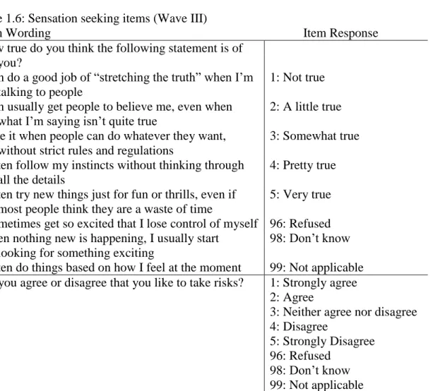
Sensation seeking: Wave III had a total of 20 items that have been used alone, or
together, to measure the sensation seeking construct. Seven of the items are modified versions of items from the Disinhibition subscale of Zuckerman’s sensation seeking scale.109 However, these
items were not presented to all respondents, only a genetic subsample.110 The other relevant items are aimed at assessing novelty-seeking and impulse control and ask respondents to use a 5-point Likert scale to report how true the statement is for them (e.g., “I often try new things just for fun or thrills, even if most people think they are a waste of time”; Table 1.6).58 Though
impulsivity can be conceptualized as containing both a sensation seeking construct and an impulse control construct, both of which can differentially predict health risk behaviors,
32
missing did not vary by respondents’ answer to the question “Do you agree or disagree that you like to take risks?” indicating that items in the scale are missing at random.
Table 1.6: Sensation seeking items (Wave III)
Item Wording Item Response
How true do you think the following statement is of you?
I can do a good job of “stretching the truth” when I’m talking to people
1: Not true I can usually get people to believe me, even when
what I’m saying isn’t quite true
2: A little true I like it when people can do whatever they want,
without strict rules and regulations
3: Somewhat true I often follow my instincts without thinking through
all the details
4: Pretty true I often try new things just for fun or thrills, even if
most people think they are a waste of time
5: Very true I sometimes get so excited that I lose control of myself 96: Refused When nothing new is happening, I usually start
looking for something exciting
98: Don’t know I often do things based on how I feel at the moment 99: Not applicable Do you agree or disagree that you like to take risks? 1: Strongly agree
2: Agree
3: Neither agree nor disagree 4: Disagree
5: Strongly Disagree 96: Refused
98: Don’t know 99: Not applicable
Confounders: In addition to the confounders listed for Aim 1, the following additional confounders were added for the Aim 2 analyses:
Wave IV respondent education: Educational attainment of the respondent in young adulthood (less than high school, high school graduate, some college, or college graduate or higher) was used as a proxy for socioeconomic status.
33
analyses using these data.61 Example items include becoming disabled, losing a family member or friend, being deployed in a combat zone, and getting arrested. Exposure to SLEs is important to control for because such exposures could increase stress biomarkers and/or depressive symptoms independent of substance use frequency. In this way, SLEs are a potential confounder of the hypothesized relationship between stress biomarkers and depressive symptoms. There appeared to be sufficient variability in the index as it ranges from 0 to 15 (median=1, SD=1.91). The correlations between the SLE index at each wave and substance use frequency at that same wave were assessed to determine if the SLE indices needed to be added as a control variable in the growth curve analyses and the correlations were not sufficiently high to warrant this.
At a physiological level, the CRP and EBV biomarkers can be influenced by many things. Looking to prior analyses of the biomarkers, we compiled a list of items that are necessary to control for when analyzing them. The same controls were used for both CRP and EBV as they are both part of the same physiological response. These potential confounders included:101,111,112
o Count of subclinical symptoms (0-3)
o Count of infectious/inflammatory diseases (0-6)
o Use of NSAID/Salicyate in the past 24 hours and/or in the past four weeks o Use of a Cox-2 inhibitor within the past four weeks
o Use of inhaled corticosteroids in the past four weeks
34
o Use of other anti-inflammatory medications o Currently pregnant
o BMI, derived from measured height and weight
o Cigarette smoking frequency measured as number of days on which a respondent smoked in the past 30 days.
o Vigorous physical activity, a dichotomous variable, assesses whether respondents, in the past 24 hours, did vigorous physical activity for long enough to get out of breath, sweat, or get their hearts thumping. A measure of recent vigorous physical activity is necessary because exercise increases inflammation in the short-term.113 Aim 2 Analyses
35 Figure 1.3: Mediation analysis framework
First, we regressed depressive symptoms at Wave IV on binge drinking frequency at Wave I, including a measure of depressive symptoms at Wave III. From this model, we got an estimate of path ‘C,’ or the total effect. Second, we regressed the AGB score from Wave III on binge drinking frequency at Wave I to get an estimate of path ‘A.’ Third, we regressed
depressive symptoms at Wave IV on binge drinking frequency from Wave I and the AGB score from Wave III, including a measure of depressive symptoms from Wave III. From this final model, we got estimates of paths ‘B’ and ‘C prime.’ We looked for the estimates of paths A, B, and C to be statistically significant and the estimate for path C prime to be zero or noticeably smaller than the estimate of path C.114 This Baron and Kenny approach to mediation has several
limitations including limiting power, not computing an estimate of the indirect effect, and missing mediating relationships that can exist even if the A, B, and C path estimates are not statistically significant.115 However, the more contemporary approach of multiplying the coefficients for the A and B paths together to get a point estimate of the indirect or mediated effect is not feasible as this then requires the use of Sobel’s z-score test to determine if the estimated effect is significantly different from zero. Unfortunately, Sobel’s test is not well suited for models with binary mediators or models with survey weights. Bootstrapping is another means to test the significance of the indirect effect estimate but is also infeasible with survey weights.82
For Aim 2, we used a combination of the Baron and Kenny and contemporary mediation
Frequency of binge drinking
M: AGB Score
Level of depressive symptoms A
C Prime: Direct Effect
36
approaches by looking to estimates of the A, B, C, and C’ paths to identify mediation but not disregarding models when the C path was not significant but the A and B paths were.
37
Potential pitfalls of this analytic approach included an inflated the type I error rate, bias, and a lack of significant results. Due to the high number of tests, the analysis plan was at risk of inflating the type I error rate. As a personal benchmark to guard for over interpretation of rare significant results among a large number of tests, the conservative Bonferroni correction for multiple tests was used as a sensitivity analysis for the results. Second, some of the hypothesized mediators were measured only in Wave IV, the same wave as the dependent variable, which could introduce some bias into the models. Simulation models have particularly highlighted problems when the direct or indirect effect is assessed in cross-sectional data.116 Fortunately, in our analytic plan, only part of the indirect effect was cross-sectional, thereby limiting the potential for bias. However, it is important to note we assumed the relationship between the hypothesized mediator and the dependent variable was instantaneous and did not vary over time.116 The third potential pitfall of the Aim 2 analyses was a lack of significant results as prior
studies have connected ingredients in marijuana with decreased levels of CRP and EBV. However, these studies were testing the effects of specific compounds in marijuana on certain cells and so we hypothesized a broader analytic framework that includes the potential stress from using marijuana would produce different results, especially for females.100,108
Sample & Power
38
clustering by primary sampling unit and region. We used Stata, version 14.0 (Stata Corp, College Station TX, 2013) for all regression and mixed effects models.
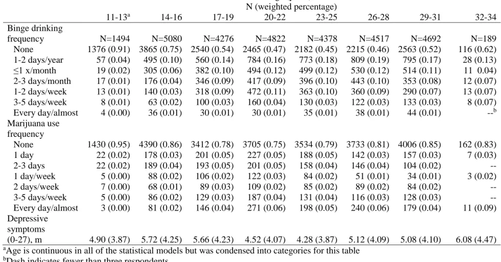
Table 1.7 below outlines the characteristics of the analytic sample for all of the variables in this project. Some points to note are first that the sample is diverse in race/ethnicity (nearly one third of the sample identifies as non-White) and parental educational attainment
(approximately one third of parents had completed college, another third completed some college and another third had a high school degree or less). Second, there is variability in our main measures. For example, 29% of males and 48% of females have elevated levels of CRP. We also see sufficiently high levels of substance use, even at Wave I. Approximately 30% of adolescent males reported binge drinking in Wave I, and this jumps up to about 60% in Waves III and IV; the increase is from 25% to 45% for females. For marijuana use, nearly 15% of males report marijuana use in Wave I, and about 30% report use by Wave III; for females, the increase is from 13% to 20%.
Table 1.7: Characteristics of the analysis sample
Characteristic Males (n=4323)
n (weighted %) or mean (SD)
Females (n=5493) n (weighted %) or mean (SD) CONTROL VARIABLES
Race/Ethnicitya (WI)
Hispanic 692 (12.2) 776 (10.7)
Black 721 (12.9) 1206 (15.4)
Asian 318 (3.6) 328 (3.3)
Native American 94 (2.5) 96 (1.9)
Other 38 (1.0) 43 (1.0)
White 2460 (67.9) 3044 (67.9)
Parental Education (WI)
< High school 475 (10.7) 687 (11.1)
High school 1023 (25.6) 1420 (28.4)
< College 1298 (30.3) 1574 (28.9)
College or higher 1527 (33.4) 1812 (31.6)
Respondent Education (WIV)
< High school 344 (8.4) 304 (6.4)