MOTIONCORRECTION FOR FMRIDATA USINGCONDITIONALTRANSITION REGIME
SWITCHINGGENERAL AUTOREGRESSIVECONDITIONALHETEROSKEDASTICITYMODELS
Teague R. Henry
A dissertation submitted to the faculty of the University of North Carolina at Chapel Hill in partial fulfillment of the requirements for the degree of Doctor of Philosophy in the Department of
Psychology and Neuroscience.
Chapel Hill 2017
c
2017
Teague R. Henry ALL RIGHTS RESERVED
ABSTRACT
TEAGUE R. HENRY: Motion Correction for fMRI data using Conditional Transition Regime Switching General Autoregressive Conditional Heteroskedasticity Models.
(Under the direction of Kathleen Gates)
For my wife, Jennifer MacCormack, my colleagues, and Cornelius F. Todd. All played an important part in making this happen.
ACKNOWLEDGMENTS
TABLE OF CONTENTS
LIST OF TABLES . . . ix
LIST OF FIGURES . . . ix
1 FMRI METHODOLOGY AND THE MOTION CONFOUND . . . 1
1.1 fMRI Data Acquisition . . . 2
1.1.1 Magnetic Resonance Imaging . . . 2
1.1.2 The BOLD time series . . . 4
1.1.3 fMRI Preprocessing . . . 4
1.1.4 fMRI Outcome Types . . . 6
1.1.5 fMRI Study Design . . . 7
1.2 Motion as a Confound . . . 8
1.2.1 Motion Correction Techniques . . . 10
1.2.2 Summary . . . 13
2 THE CTRS-GARCH MOTION CORRECTION METHOD. . . 14
2.1 Time Series and fMRI . . . 14
2.1.1 Autoregressive and Moving Average Time Series . . . 14
2.1.2 Univariate GARCH . . . 15
2.1.3 Multivariate GARCH . . . 16
2.1.4 Regime Switching Multivariate GARCH . . . 18
2.1.5 Regime Switching . . . 18
2.1.6 Regime Switching Dynamic Correlation GARCH . . . 19
2.1.7 The CTRS-GARCH model . . . 20
2.2 The CTRS-GARCH Model Specification . . . 22
2.2.1 GARCH components . . . 25
2.2.2 Estimation of State Specific Correlation Matrices . . . 29
2.2.3 Estimation of the Static Transition MatrixΠ . . . 30
2.2.4 Estimation of the effect ofxon regime change . . . 31
2.2.5 Estimation of posterior probabilities of regime membership . . . 32
2.2.6 The EM Algorithm . . . 32
3 SIMULATIONS . . . 34
3.0.1 Simulation of Motion . . . 34
3.0.2 Generating the True Signal . . . 35
3.0.3 The Simulated Effect of Motion . . . 39
3.0.4 Scrambling the True Signal Matrices . . . 40
3.0.5 Combining True Signal and Motion Correlation Matrices . . . 41
3.0.6 Simulating the fMRI time series . . . 42
3.1 Simulation Conditions . . . 43
3.1.1 Simulation Set 1: Discrete Motion Artifacts . . . 43
3.1.2 Simulation Set 2: Continuous Motion Artifact . . . 44
3.1.3 Overview of the Simulation Setup. . . 44
3.1.4 Analysis of the Simulated Data . . . 46
3.2 Results . . . 47
3.2.1 Discrete Motion Artifact . . . 47
3.2.2 Continuous Motion Artifact Results . . . 53
3.2.3 Summary and Conclusion for Simulation Studies. . . 58
4 ANALYSIS OF EMPIRICAL DATA . . . 60
4.1 Overview . . . 60
4.2 Analysis of Motion in Empirical Data . . . 60
4.3.1 Data Acquisition and Preprocessing. . . 61
4.4 Analysis and Results . . . 62
4.4.1 Between Diagnostic Category Differences. . . 66
4.5 Summary . . . 69
5 DISCUSSION . . . 71
REFERENCES. . . 75
LIST OF TABLES
4.1 Frequency of Clinical Group by Gender. TDC is Typically Developing Control, ASD is Autism Spectrum Disorder, Inattentive is Inattentive type ADHD and Combined is Combined type ADHD . . . 62 4.2 Demographic Descriptives . . . 62 4.3 Overall pairwise mean differences between in the Fisher-Z transformed correlations of
LIST OF FIGURES
1.1 Timeseries of BOLD Signal and Frame Displacement for an adolescent with autism. higher values of frame displacement indicates higher amounts of motion. Note the large drop in BOLD signal for two of the occasions of motion, as well as the increase in volatility
during the large amount of motion during the middle of the scan. . . 9
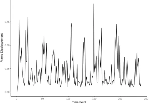
3.1 Example Simulated Frame Displacement . . . 36
3.2 Example Empirical Frame Displacement . . . 36
3.3 10 ROI connectivity networks. Thicker lines represent higher edge weights. . . 37
3.4 15 ROI connectivity networks. Thicker lines represent higher edge weights. . . 38
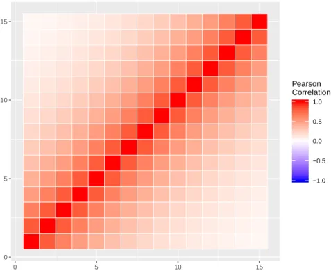
3.5 10 ROI Correlation Matrices. . . 39
3.6 15 ROI Correlation Matrices. . . 39
3.7 Simulated Motion Correlation Matrix . . . 40
3.8 15 ROI Scrambled Correlation Matrices. . . 41
3.9 10 ROI Scrambled Correlation Matrices. . . 41
3.10 15 ROI High Signal Matrix contaminated at 70% Motion (ρ=.8) . . . 42
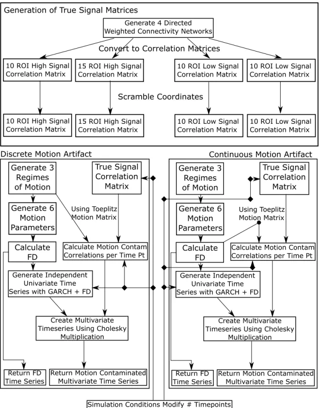
3.11 A simple visual depiction of the simulation structure. The lower windows are per dataset. Within a set of conditions, this would be repeated 100 times. . . 45
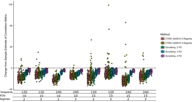
3.12 Change in the estimate of the true signal correlation matrix for the High Signal Discrete Motion Artifact Condition Set. Note that on average, all presented methods improve the estimate of the true signal correlation matrix, as the majority of the points are below the 0 line. In conditions with more information (more time points, fewer ROIs), 2 regime CTRS-GARCH tends to outperform all other methods. Finally, 3 regime CTRS-CTRS-GARCH appears to have a tendency to produce outliers, as evidenced by datapoints with extremely bad estimates of the true signal correlation matrix. . . 48
3.13 Change in the estimate of the true signal correlation matrix for the Low Signal Discrete Motion Artifact Condition Set. This condition set indicates considerably more variance in the relative improvement, with more iterations that resulted in poor estimates of the true signal correlation , particularly for the CTRS-GARCH approaches. These issues appear to be most prevalent at low information conditions, and at higher information conditions, 2 regime CTRS-GARCH tends to either meet or outperform the most conservative scrubbing approach (.2 FD). . . 49
3.14 Comparison of the 2 regime CTRS-GARCH solution to Scrubbing at .2 and .3 FD within a simulation trial for High Signal Discrete Motion Artifact Conditions. Negative numbers indicate that the CTRS-GARCH solution was superior to the scrubbing solution. Note that on average, 2 regime CTRS-GARCH outperformed scrubbing at both .2 and .3 FD, with the majority of trials indicating that the CTRS-GARCH solution was superior. Again, in higher information conditions, CTRS-GARCH showed clear advantage, whereas for lower information conditions, CTRS-GARCH showed less of an advantage. Note too the large shift in results when looking at .2 FD vs .3 FD scrubbing. . . 51 3.15 Comparison of the 2 regime CTRS-GARCH solution to Scrubbing at .2 and .3 FD within
a simulation trial for Low Signal Discrete Motion Artifact Conditions. Negative numbers in-dicate that the CTRS-GARCH solution was superior to the scrubbing solution. These results indicate that the conservative scrubbing threshold of .2 was either equivalent or superior to 2 regime CTRS-GARCH in almost every condition, where as .3 FD scrubbing performed slightly worse than 2 regime CTRS-GARCH in almost every condition. As expected, the places were 2 regime CTRS-GARCH outperformed scrubbing were the high information conditions (240 time points, 2 regimes), however this improvement was small when com-pared to the high signal condition (3-5 units vs. 20-30 units.) . . . 52 3.16 Change in the estimate of the true signal correlation matrix for the High Signal
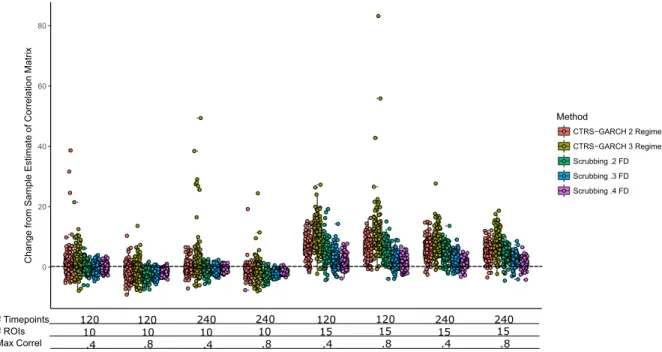
Continu-ous Motion Artifact Condition Set. Here, we see that in the 15 ROI condition set, all motion correction methods perform worse than the raw data estimate, while in the 10 ROI condition set, scrubbing is the only method that has the tendency to improve the estimation of the true correlation matrix. In all cases, the estimates from CTRS-GARCH are more variable than scrubbing, and are more likely to result in worse estimates of the true correlation matrix. . . 54 3.17 Change in the estimate of the true signal correlation matrix for the Low Signal
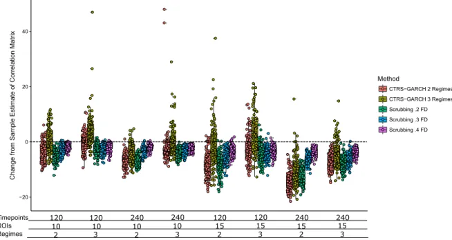
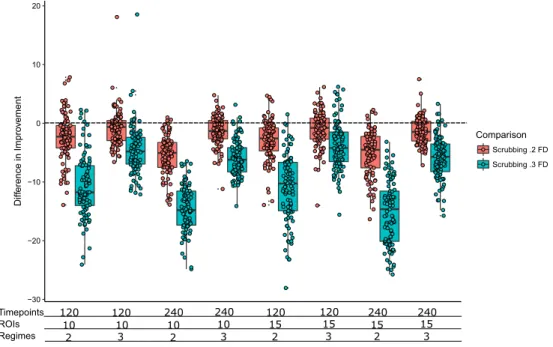
Contin-uous Motion Artifact Condition Set. CTRS-GARCH, in all conditions, resulted in worse estimates of the true correlation matrix than the raw data estimates. Additionally, scrubbing appears to have no, or a slightly negative, effect on the quality of the estimate, as evidenced by the zero centering of the scrubbing distributions. . . 55 3.18 Comparison of the improvement over the uncorrected data from 2 Regime CTRS-GARCH
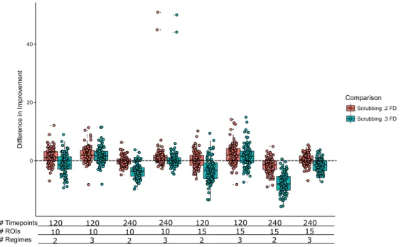
to Scrubbing at .2 FD and .3 FD in the High Signal Continuous Motion Artifact Condition Set. Negative values indicate CTRS-GARCH performing better than the comparison. Note that in all cases, scrubbing out performs CTRS-GARCH. Notably, scrubbing at .3 FD tends to outperform CTRS-GARCH more than scrubbing at .2 FD. This is due to the previous findings that harsh scrubbing results in a lower quality estimate of the true signal correlation matrix than the uncorrected data estimate. . . 56 3.19 Comparison of the improvement over the uncorrected data from 2 Regime CTRS-GARCH
4.1 Plot of the Uncorrected QC-RSFCs with the Corrected QC-RSFCs for each motion cor-rection method. The line represents no change in the QC-RSFCs. Below the line represents an improvement in QC-RSFCs while above represents a increase in the association with motion. Note that for higher uncorrected QC-RSFCs, scrubbing either improves or leaves unchanged the QC-RSFCs, while at low uncorrected QC-RSFCs, scrubbing increases the QC-RSFCs. Both CTRS-GARCH applications tend to improve QC-RSFCs dramatically. . . 64 4.2 Plot of the Uncorrected QC-RSFCs with the Corrected QC-RSFCs for CTRS-GARCH
methods. The line represents no change in the QC-RSFCs. Below the line represents an improvement in QC-RSFCs while above represents a increase in the association with motion. 65 4.3 The average change from the uncorrected QC-RSFC (Fisher Z transformed) by diagnostic
category and motion correction method (.2 FD is scrubbing at .2 FD, 2 regimes is 2 regime CTRS-GARCH, etc.). Note the similarities in effect for the TDC, ASD and ADHD-C, and that the main differences are in the ADHD-I group. . . 67 4.4 QC-RSFC comparisons for the ADHD-I subgroup. Note the larger number of points
above the diagonal line, denoting an increase in the correlation with motion. . . 68 4.5 QC-RSFC comparisons for the TDC subgroup. Note the larger range of correlations in
comparison with the ADHD-I, as well as a greater concentration of those correlations in the upper area of the uncorrected QC-RSFC. . . 69
1 FMRI METHODOLOGY AND THE MOTION CONFOUND
Functional Magnetic Resonance Imaging, or fMRI, is a technical methodology that allows re-searchers to investigate so called functionalhypotheses regarding brain activity. These hypotheses can be termed functional in nature as fMRI nominally measures an analog of neural activity in the brain. This differs from structural MRI, as structural MRI does not assess the active functioning of the brain, and rather provides an image of the anatomical structure. fMRI methodology has been used to study everything from the functioning of typical adults (Biswal, Yetkin, Haughton, & Hyde 1995) to task based performance of children with autism (Gomot et al. 2006), and a full review of the uses of fMRI is beyond the scope of this dissertation. Instead, this dissertation will focus on a particular issue of fMRI data collection that cuts across every application, that of motion of the participant when the fMRI data are being collected. Motion distorts the data, raising the chance of false positive findings, and is a particularly salient concern for applications regarding children and individuals with clinical disorders such as autism.
There are a variety of motion correction techniques, and this dissertation will review several of them, however the purpose of this dissertation is to introduce a new motion correction technique, the Conditional Transition Regime Switching Generalized Autoregressive Conditional Heteroskedastic-ity model (CTRS-GARCH), that is designed to target the particular issue of datasets with high motion where functional connectivity is the outcome under study. This method effectively breaks down the fMRI time series into a series of correlation matrices, and accounts for how motion affects the differ-ences between these correlation matrices. For the substantive user of this motion correction method, the CTRS-GARCH can either provide a motion corrected correlation matrix for each subject, or a motion corrected time series depending on the needs of the researcher.
generalized autoregressive conditional heteroskedasticity models (GARCH) will be reviewed. Fourth, the CTRS-GARCH model will be analytically derived and a method of estimation will be outlined. Fifth, a set of simulations will be presented comparing the CTRS-GARCH to other commonly used motion correction methods. Sixth, and finally, an empirical study will be presented, again comparing the performance of the CTRS-GARCH with other commonly used methods for motion correction. 1.1 fMRI Data Acquisition
fMRI stands for functional magnetic resonance imaging, and this technique of data acquisition seeks to acquire images that represent the functioning of various regions of the brain. While the physics of the data acquisition are complex, and a full treatment is beyond the scope of this disser-tation, it is useful to provide a brief overview of how fMRI data are acquired, and in particular what data are acquired, as the actual signal required is not the true neurological functioning of the brain, but rather a proxy based on blood oxygen flow.
1.1.1 Magnetic Resonance Imaging
Magnetic resonance imaging, of which fMRI is a particular subtype, is a technology that allows researchers to form 3D images of solid objects, using an interaction between a strong magnetic field and radiofrequency pulses (Huettel, Song, & McCarthy 2014). The process by which these images are collected is fairly straightforward.
To begin, an MRI scanner contains a large superconducting electromagnet, used to generate a static magnetic field of anywhere between 1.5 Tesla to 11 Tesla, with the most common field strengths for fMRI on humans being 3T and 7T. This magnetic field aligns the hydrogen atoms in the human body, most of which are contained in the water that makes up the majority of the volume of the human body, into a low energy state (specifically, the static magnetic field aligns the spin states of protons in atoms to a parallel spin, which is lower energy). The MRI scanner also contains radiofrequency coils. Once the magnetic field has aligned the protons, the radiofrequency coils release a series of pulses of electromagnetic waves. These waves are absorbed by a percentage of the aligned protons (in the case of fMRI the aligned protons are concentrated in deoxygenated blood), which knocks these protons into a higher energy state, where the spin is not aligned to the magnetic field, and when the pulse ends, the protons that were in a high energy state fall (the analogy here of potential energy and an object
falling into a gravity well is appropriate) into the low energy aligned spin state. This “fall” releases an electromagnetic wave that can be detected by the radiofrequency coils (Huettel et al. 2014).
This release of energy has no spatial information because as the protons are uniformly aligned by the static magnetic field, and the radiofrequency pulse is also uniform across the subject. The final piece of MRI imaging is the gradient coils. These coils modify the magnetic field by emitting a series of pulses over the course of the scan (the pulse sequence) so that the magnetic field is no longer uniform across the entire subject. This lack of uniformity allows the scanner to calculate where a particular signal is coming from, so it is the gradient coils that allow MRI imaging to have the necessary spatial information.
The type of image, be it structural, functional, chemical or dynamic is determined by the pulse se-quence of the gradient coils. By changing the pulse sese-quence, different parts of the subjects anatomy are aligned to the magnetic field differently. These differences in alignment, and the resulting dif-ferences in images are calledcontrasts. Utilizing different contrasts allows the researcher to obtain different types of images. For example, theT1 contrast is used to examine the structural differences
between grey matter and white matter in the brain (Huettel et al. 2014). The T2 contrast picks up
on areas that contain large amounts of fluids. For fMRI applications however, the most important contrast is theT2∗contrast, which best shows the presence or absence of deoxygenated blood (Huettel et al. 2014).
acting in milliseconds, while BOLD operates over seconds (Logothetis 2008). Moving forward, this distinction is important to keep in mind as the specifics of fMRI study design are discussed.
1.1.2 The BOLD time series
As the scanner is run on a subject the fMRI image is built up in a series of slices. These slices are produced as a product of the pulse sequence, and are combined, and then corrected, to form a voxel by voxel image of the subject’s brain at a given time point. Thevoxelis the smallest unit of analysis in any MRI study. Avoxelis a 3-dimensional space, that can be in the order of millimeters to a side, or centimeters, where per time point a single number representing the signal strength within that voxel is assigned. In the case of fMRI, this signal is the BOLD signal, and so the number assigned to each voxel at a time point represents the amount of deoxygenated blood in that voxel, and by proxy the neuronal activity in that voxel.
As was mentioned above, an MRI image is a 3-dimensional dataset. With an fMRI image, we have an additional dimension, that of time. In fMRI, BOLD response is collected per voxel per time point. The interval between time points can be anywhere between less than a second and more than five seconds, with a two second interval being a common choice. Smaller between time point intervals result in less spatial resolution, and a more noisy dataset, while longer time intervals increase spatial resolution, but of course decrease the temporal resolution. BOLD response after neuronal activity is of the order of several seconds (Huettel et al. 2014), making these time intervals consistent with the process under observation.
While the data that come directly out of a scanning session can be conceptualized as a multivariate time series, it is in fact unusable for analysis in its raw form. Raw data directly from the scanner are beset by gross motion artifacts, as well as a variety of physiological noise signals, which need to be removed before any analysis can be taken place. Before any analysis can be done the raw data must be preprocessed.
1.1.3 fMRI Preprocessing
Preprocessing MRI data is a complex endeavor, and like many aspects of MRI overall, a detailed treatment is beyond the scope of this dissertation. Aspects of preprocessing include quality assurance, where researchers examine the images to ensure that no scan artifacts are present, as well as the
application of various filters to remove physiological noise, such as the cyclical effect of breathing from the data (Huettel et al. 2014). The one aspect of preprocessing that will be discussed here is motion correction.
Motion is one of the most pernicious causes of data distortion in any MRI study (Power, Barnes, Snyder, Schlaggar, & Petersen 2011). A full treatment of the effects of motion on fMRI outcomes is presented later in this chapter, but for now we can focus on the more obvious effects of motion. The most obvious effect of motion is the shift in voxel location that occurs. Very small movements, such as 5mm, can result in the locations of the voxels being shifted dramatically (Huettel et al. 2014). This shift can cause significant differences in signal strength, and given that the head can and will move multiple times during a scanning session, the accumulated distortions can result in nearly unusable data.
To combat this,coregistrationbyrigid-body transformationis used (Huettel et al. 2014, Pg. 304). Coregistration refers to the aligning of two images, which is typically applied recursively to each time point, resulting in a final set of images that have been re-aligned to match one another. Rigid-body transformation is the process of performing the realignment, which is made simpler due to the fact that the head and brain do not change shape over the course of the scan. In order to perform this realignment, the motion parameters, namely movement in all three directions, as well as rotation in all three dimensions need to be estimated. There are a variety of techniques with which to estimate these parameters, and a different technique is used for each popular preprocessing software package. For example, FSL (FMRIB (Functional MRI of the Brain) Software Library) uses an algorithm termed MC-FLIRT (Motion Correction - FMRIB’s Linear Image Registration Tool); (Jenkinson, Bannister, Brady, & Smith 2002), while SPM (Statistical Parametric Mapping) uses an unnamed coregistration technique (Penny, Friston, Ashburner, & Nichols 2006).
ROI selection
As an important aside, it is often the case that a researcher does not want to work with voxel level data. Regions of Interest (ROI) analysis for fMRI data in particular can provide an alternative. ROIs are sets of (usually) spatially contiguous voxels that are aggregated in some way. This aggregation can be done using a simple mean, or a more complex spatial weighting scheme, but the idea remains the same, and that is that the aggregate signal from the set of voxels is a more reliable measure of functional connectivity in that region. The sets of voxels that make up each ROI can be determined from a preexisting atlas, such as the Automated Anatomical Labeling atlas (AAL; Tzourio-Mazoyer et al. (2002)), the Harvard-Oxford atlas (HO; Desikan et al. (2006)) or the canonical Brodmann atlas Brodmann (1909). Alternatively, ROI maps can be generated on a per subject basis by examining functional connectivity between voxels and grouping voxels accordingly, or by using a cognitive task and determining the set of voxels that activate during that task. There are several algorithms for doing this, one example is the Craddock atlas generator (Craddock, James, Holtzheimer, Hu, & Mayberg 2012).
1.1.4 fMRI Outcome Types
While the true output of an fMRI session is a multivariate time series of the estimated BOLD response, we can divide the outcomes of interest into two broad camps, that ofsite based activation, or that of functional connectivity. Site based activation refers to the presence or absence of a signal at a particular region of interest, and is used to infer activation of that brain region. For example, if a participant is given a visual stimuli task, the V1 area of the primary visual cortex shows a increased BOLD response in that region. This would suggest that there is neurological activity in that region. While these outcomes have been of interest in the past, and are indeed still of interest for many task based studies, in this dissertation we focus on functional connectivity.
Functional connectivity attempts to measure coactivation of regions within the brain. This can be done with seed correlation (Huettel et al. 2014), where an initial seed voxel is designated, and all other voxels are then correlated with that seed voxel, to determine the functional connectivity between the seed and other areas. Alternatively, if one is working at a larger spatial scale, one can calculate a correlation matrix between all regions of interest (ROIs), which can establish a functional
connectivity map.
The covariance matrix, or the equivalent correlation matrix of the pairwise relations between ROIs is the most common data analysis object in functional connectivity analysis. While there are several methods that use the raw time series to attempt to construct a causal relation network, such as SEM approaches (J. Kim, Zhu, Chang, Bentler, & Ernst 2007) or dynamic causal modeling (Friston, Harrison, & Penny 2003), the most common approach to functional connectivity is to use the observed time series to calculate the pairwise correlation matrix, possibly use this matrix to calculate the partial correlation matrix, and to treat these matrices as the “network” of functional connectivity (Smith, Menon, & Thompson 2011). From this network, a variety of network statistics can be calculated and inferential procedures can be performed (Bullmore & Sporns 2009). This reliance on the correlation matrix for functional connectivity requires the ability to robustly estimate the true correlation matrix of the fMRI signal, uncontaminated by any sort of noise process.
Of particular note is the idea of dynamic functional connectivity (Hutchison et al. 2013). In previ-ous years, functional connectivity has been calculated in a static fashion, treating whatever measure of functional connectivity calculated as the same across an entire block of time within the overall acqui-sition. Recently there has been a movement towards a more dynamic view of functional connectivity as changing over the course of acquisition. Methods to assess this include sliding windows (Hindriks et al. 2016), multivariate GARCH models (Lindquist, Xu, Nebel, & Caffo 2014), independent vec-tor analysis techniques (Ma, Calhoun, Phlypo, & Adali 2014) and state-space modeling (Molenaar, Beltz, Gates, & Wilson 2016).
1.1.5 fMRI Study Design
(Huettel et al. 2014), where researchers have ana prioriidea of the regions or voxels that are active during a particular task, and can describe a hypothesis that then can be tested.
Resting state data, which originated in the seminal paper of Biswal et al. (1995), involves having the subject simply rest in the scanner. Resting state data can provide a look at the general functional connectivity of a subject, and is often the data used to examine between-subject differences in func-tional connectivity. That being said, resting state fMRI is a data-driven affair, where there is a typical lack of hypotheses regarding the data (Huettel et al. 2014).
1.2 Motion as a Confound
One of the central themes of this dissertation is that motion has wide ranging and disruptive effects on fMRI data. As was mentioned above, motion during a scan physically changes the positioning of the voxels. During preprocessing this is corrected using coregistration and realignment. However, motion also disrupts the homogeneity of the magnetic field in the MRI scanner, and the effects of motion cannot be completely corrected using realignment.
This issue was first presented in the neuroimaging literature in 2011 and 2012 by three indepen-dent research groups, Power, Barnes, et al. (2011), Satterthwaite et al. (2012) and van Dijk, Sabuncu, & Buckner (2011). The general conclusion from all three of these groups is that small amounts of mo-tion cause systematic differences in funcmo-tional connectivity, that could be misinterpreted as between group differences, or other substantive findings. Specifically, Power, Barnes, et al. (2011) found that spatially distant regions had their correlation reduced by movement, while spatially close regions had their correlation increased by movement, and this general effect had a large degree of variance both within and between subjects. Both Satterthwaite et al. (2012) and van Dijk et al. (2011) had similar findings to Power, Barnes, et al. (2011). Furthermore, this distortion in the fMRI signal was found to occur during and immediately after the movement. As Power, Barnes, et al. (2011) illustrates with an example, an individual with a single severe movement will have better quality data overall than an individual with continuous micromovements, or small movements that occur in a matter of seconds, with individuals occasionally returning to the place of origin. It is hard to overstate the severity of the motion artifact. Power et al. (2014) states that the artifact caused by even small amounts of motion could result in spurious findings, and several studies have already been reevaluated to ensure that
their findings are robust to the motion artifact (e.g. Fair et al. (2012)). Figure 1.1 below shows the time series of 5 ROIs from an adolescent with autism spectrum disorder, along with the time series of frame displacement, a measure of motion that will be explained later in this dissertation.
BOLD Signal
FD
0 100 200 300
−30 −20 −10 0 10
0 1 2
Time Point
V
alues
Figure 1.1: Timeseries of BOLD Signal and Frame Displacement for an adolescent with autism. higher values of frame displacement indicates higher amounts of motion. Note the large drop in BOLD signal for two of the occasions of motion, as well as the increase in volatility during the large amount of motion during the middle of the scan.
With the problems presented by motion artifacts so revealed there has been an increased interest in motion correction techniques that can be used in tandem with the rigid-body correction already present in preprocessing. In the following section, we examine in detail the two most popular meth-ods, 24-parameter regression and scrubbing.
1.2.1 Motion Correction Techniques
24 Parameter Motion Regression
24 parameter motion regression was originally proposed as a solution to the motion artifact by Friston, Williams, Howard, Frackowiak, & Turner (1996). This regression takes the 6 motion pa-rameters, translation in the X, Y and Z direction, as well as the pitch P, roll R and yaw W for rotation, and uses them and time lagged expansions to attempt to regress the effects of motion out of the fMRI signal. The 24 parameter regression which incorporates 2 time points (Power et al. 2014) is as follows:
St∗ =St−Sˆt (1.1)
ˆ
St =β0+β1Xt+β2Xt2 +β3Xt−1+β4Xt2−1+β5Yt+· · ·+β24Wt2−1. (1.2)
WhereSt∗is the corrected signal for theSvoxel andStis the original value for theSvoxel at time
pointt. While at first blush, this technique appears to be promising for extracting the motion artifact, evaluations of its performance suggest that it is highly inefficient at removing the effect of motion (Power, Barnes, et al. 2011; Power et al. 2014). Additionally, increasing the time lagged information from one lagged time point to two and three does improve the extraction of the motion artifact, but only slightly (Power et al. 2014). This lack of performance is likely due to the assumption of homogeneity inherent in the regression approach. In this approach, motion is considered to have the same effect on each voxel. However, this is likely not the case, as the effect of motion on alignment potential is not homogeneous (Power, Barnes, et al. 2011; Huettel et al. 2014).
It is also worthwhile to note that a common regression technique used in preprocessing, global signal regression, is highly effective at reducing the effect of motion (Power et al. 2014). However, global signal regression has the potential to distort the fMRI signal independently of motion. Murphy,
Birn, Handwerker, Jones, & Bandettini (2009) and Saad et al. (2012) indicate that the use of global signal regression can induce negative correlations between voxels. The efficacy of global signal re-gression is an ongoing area of research, however, given that it is not a dedicated motion correction technique that potentially has additional consequences suggests that it is not an ideal option for cor-recting the effect of motion.
Theoretically, regressing the effect of motion out of the time series is an attractive option from several views. The first being that the regression preserves the temporal nature of the time series. As opposed to scrubbing, the next correction technique to be discussed, regression does not remove time points wholesale, but rather attempts to remove the portion of signal that motion account for. If this was successful, it would leave an intact time series, so that both static functional connectivity analysis could be conducted, but more importantly dynamic functional connectivity (which ideally needs an intact time series) could be performed. Furthermore, the use of regression on high motion populations, such as pediatric populations, or individuals with clinical disorders such as autism or ADHD would be ideal, as it would not result in the wholesale loss of time points that scrubbing results in. However, as regression is not effective at removing the motion artifact, this approach is not valid, but the advantages of a regression approach should be kept in mind as we continue the discussion of motion correction techniques.
Scrubbing
Scrubbing, or the wholesale removal of points above a particular threshold of motion, has been shown to be effective at significantly reducing the motion artifact (Power, Barnes, et al. 2011; Power et al. 2014; Satterthwaite et al. 2013a). Typically, to use scrubbing a single value that represents the aggregate level of movement at a given time point is calculated. While a mean of the motion param-eters can certainly be used, a popular alternative is that of frame displacement. Frame displacement has several definitions, but one of the most widely used comes from Power, Barnes, et al. (2011), as follows:
Where the motion parameters are as before, and∆t:t−1 is the difference between the values of a
given parameter fromt−1tot. Frame displacement provides an aggregate look at the magnitude of the movement from one time point to the next. By convention, F D1 is 0. As a measure of motion,
frame displacement is appropriate given the lack of efficacy of the regression approaches to motion correction.
Once frame displacement has been calculated, scrubbing is a simple matter of removing time points based on some rule involving frame displacement. A common choice is a simple threshold, where any time points that exhibit over, for example, a frame displacement of .2mm for a fairly stringent threshold, or a frame displacement of .5mm for a more liberal threshold (Power, Barnes, et al. 2011). Another approach is to remove both the time points that exceed the threshold, and a number of time points afterwards. The reasoning of this is that the effect of motion is not only apparent at the time point of the movement, but also in the time points that follow, often for several tens of seconds (Power et al. 2014). An alternative to frame displacement is that of DVARS, which measures the change in the variance of an fMRI signal (Smyser et al. 2010). It is important to note that DVARS is not a measure of motion, but rather is a measure of the stability of the fMRI signal. As motion does greatly effect the variance of the fMRI signal, DVARS is related to motion, but could also be confounded with a dynamic fMRI signal that changes systematically.
Several studies have shown the efficacy of the scrubbing approach. Power et al. (2014) shows that when applied to cohorts of adults who exhibited different levels of mean FD, and had significant dif-ferences in their functional connectivity (which, theoretically, they had no reason to have), scrubbing could reduce those differences down to below significance. Satterthwaite et al. (2013b) uses spike regression, which is functionally equivalent to scrubbing, and can be implemented simultaneously to a regression approach. Their approach showed a marked improvement in the motion artifact.
While scrubbing is undoubtedly efficient at removing the motion artifact, there are a couple in-herent problems with the approach. First, and most obviously, scrubbing removes time points, which forces researchers to use the reduced dataset, as imputation is not an option given that there is little information as to a correct imputation model. The use of the reduced dataset leads to reduced power for any statistical test, just on the basis of sample size reduction. Second, in populations with high
movement such as children and individuals with clinical disorders such as ADHD or autism, the num-ber of time points removed could render a subject unusable, and in the case of many clinical disorders each subject is a considerable investment on the part of the researcher.
On the other hand, scrubbing has several advantages over other approaches. The first is that it is inherently non-parametric. The functional form of the motion artifact is not a factor in scrubbing, as any time points that exhibit excess motion are removed. The second advantage is that it provides a very clear picture of which time points are problematic.
1.2.2 Summary
2 THE CTRS-GARCH MOTION CORRECTION METHOD
2.1 Time Series and fMRI
While functional connectivity analyses typically result in a correlation matrix as output, fMRI data at its core is a multivariate time series. A time series, simply put is any set of data that is indexed by time, and has some sort of ordered inter-dependency. While this dissertation deals with a type of model that acts on time dependent variances, it is useful as a grounding to briefly describe the two most common types of dependence in univariate time series modeling, and to discuss difficulties with the multivariate generalization of these dependences. After this overview, we will move to a discussion of the generalized autoregressive conditional heteroskedasticity model (GARCH; Engle 1982), which forms the core of the model developed in this dissertation.
2.1.1 Autoregressive and Moving Average Time Series
The most common forms of dependency modeled in time series data are those ofautoregressive effects andmoving averageeffects (Hamilton 1994). Consider the following:ytis indexed byt, with
t ∈1, . . . , T. An autoregressive effect of lag 1 (with a 0 intercept) would be described by:
yt=βyt−1+t. (2.1)
Whereβ is the autoregressive effect, andtare i.i.d error terms with some distribution (typically
normal).
A moving average model (again, with a 0 intercept) would be described as :
yt=θt−1+t. (2.2)
Whereθis the moving average effect.
discussed here. Of importance however is the rapid increase in the number of parameters to estimate in a wholly unrestricted multivariate AR or MA type model. For example, in an autoregressive lag 1 model that is bivariate, there are four potential lagged effects, the autoregressive effect of each variable on its next time point, and the cross lag effect of each variable on each other. This model complexity rapidly increases as more dimensions or lags are added to the data.
With the basic form of dependence so described, we can move onto a discussion of GARCH models, which form the core of the CTRS-GARCH model developed in this dissertation.
2.1.2 Univariate GARCH
The generalized autoregressive conditional heteroskedasticity model or GARCH, was first intro-duced by Bollerslev (1986) as a model to investigate returns on stock prices. Fundamentally, instead of examining the change in the expected value of a process, the GARCH model examines changes in the variance of a process, and is related to a moving average process. GARCH type models are useful when the pattern of change one expects to see in a process results in heteroskedastic errors, or changes in the variance of the process over time. Expected value models often make the assumption of conditional homoskedasticity, and so would be inappropriate for processes with changing variances or covariances. The specification for a GARCH(1,1) model is as follows:
yt=
p
htt (2.3)
ht=α+βht−12t−1+θht−1. (2.4)
Wherehtis the variance of the time series at timet,βis the effect of the empirical residual at lag,
andθis the effect of the estimated lagged variancethas a variance of 1. Engle (2001) describes the
2.1.3 Multivariate GARCH
Typically, the goal in fMRI for functional connectivity is to perform analysis on the correlation or covariance matrix of the fMRI time series, given the assumption that these matrices map onto the functional relations between regions of interest. As a covariance is a generalization of the variance term for multivariate distributions, a multivariate GARCH is ideal for the analysis of fMRI data. The general specification is similar to a univariate GARCH model:
yt=H1t/2t (2.5)
Whereyt is ap dimensional random variable, is a pdimensional random variable with a
co-variance matrix ofIp, andHtis ap×ppositive definite matrix, that acts as the covariance matrix of yt.
One of the most general specifications of a multivariate GARCH model is the vector error cor-rection or VEC model of Bollerslev, Engle, & Wooldridge (1988), in which each element of theHt
matrix is a linear function of the lagged squared error terms and cross products, as well as the lagged elements ofHt. The specification is as follows:
Ht=ω+αvech(Ht−1)vech(t−10t−1) +βvech(Ht−1). (2.6)
Where vech(·) is a vector stacking operation that operates on the upper triangular portion of a matrix, α and β are square matrices of parameters of order p(p −1)/2, and ω is a p(p − 1)/2
vector of parameters. This model is not computationally tractable for dimensions of over 2 or 3, so restrictions must be put in place. One model with such restrictions that deserves a description in this dissertation is the dynamic correlation model (DCC) of Engle (2002). This model has been used in fMRI analysis by Lindquist et al. (2014), and indeed is the first and only GARCH type model to have found use on fMRI data.
The DCC is a highly constrained multivariate GARCH that decomposes the covariance matrix of
the time series as follows:
Cov(yt) =Ht. (2.7)
Ht=DtΓtDt. (2.8)
WhereDtis anp×pdiagonal matrix with the standard deviations of each dimension of the time
series on the diagonal, andΓtis a correlation matrix.
The DCC then proposes that each diagonal element ofD2t, the matrix that contains the variances of each dimension, follows a univariate GARCH model with the following specifications:
D2t =diag(ω) +diag(α)diag(yt−1y0t−1) +diag(β)D 2
t−1. (2.9)
Where nowω,α,β are allp×1vectors of parameters, diag is a function that when applied to a vector turns that vector into a diagonal square matrix with 0s off-diagonal, and when applied to a square matrix, returns only the diagonal elements in a diagonal matrix. is the Hadamard product, or elementwise multiplication. At the level of individual variances, the expression is as follows:
d2(p)t=ω(p)+α(p)d2(p)t−1 2
(p)t−1+β(p)d2(p)t−1 (2.10)
DCC is a univariate GARCH type model for each individual correlation inΓt. Each off-diagonal
element in Γt depends on the estimated value of that element Γt−1 and the observed cross residual
element in t−10t−1. This reduces the total number of parameters to be estimate to 2p2 +p. The
account cross lagged relations between correlations. As this dissertation focuses on the effect that motion has on the whole functional connectivity network, an effect that is thought to be complex and not easily parameterized, a different approach than the DCC would be needed. This approach can be found in the regime switching multivariate GARCH model of Pelletier (2006).
2.1.4 Regime Switching Multivariate GARCH
The two previously discussed models, the VEC of Bollerslev et al. (1988) and the DCC of Engle (2002) both proposed smoothly varying correlations and variances across time. However the cost of those proposals was untenable complexity in the case of the VEC model, or harsh restrictions in the case of the DCC. In the application of this dissertation, the concern is not to completely reproduce the complex data generating process that results from motion artifacts, but to rather approximate the effect of motion on the underlying truefunctional connectivity correlation matrix to some high degree. This approximation can be achieved with a regime switching multivariate GARCH. This approach is, in brief, a Markov processed finite mixture modeling approach that allows the effect of motion to occur not as a continuous process, but rather as a series of shifts in the correlation matrix. These shifts can then persist over several time points. This reflects the persistent effect of motion on functional connectivity after motion has ceased, as well as reflecting the notion that an individual likely is in a different mental state while moving. Before we go into the details of the regime switching multivariate GARCH, the idea of regime switching will be briefly explained.
2.1.5 Regime Switching
Regime switching in time series analysis is a general concept that can be applied to almost any time ordered data set and model (C.-J. Kim & Nelson 1999). Regime switching can be illustrated with a mean switching autoregressive model:
yt=µt+βyt−1 +t. (2.11)
µt=µSt=s. (2.12)
t∼N(0, σ2). (2.13)
WhereStis a discrete regime state, with possible values s = {1, . . . , K}, andµis the mean of
the process that changes with the state. In the vast majority of applications of regime switching the state at any time point is not known. In the model described in Equations 2.11-2.13, the mean of the univariate time series exhibits a regime switching structure, which is to say that during a particular state, the mean of the process does not change, but when the state transitions to a different value the mean then changes. In general, transition from state to state, or the regime switching is a first order Markov process (C.-J. Kim & Nelson 1999), which means:
P(St =s|y1, . . . , yt, S1, . . . , St−1) =P(St=s|yt, St−1). (2.14)
Simply, that the probability of transitioning into a state conditioned on the time series up to the point in question is equivalent to the probability of transitioning to a state conditioned on the current time point’s value and previous time point’s state. The transition probabilities are organized into a transition matrix, denoted usually as Π, where the entry πij denotes P(St = i|St−1 = j). In
its simplest form the transition matrix is time invariant, however there are modifications that allow for covariates to affect the transition probabilities (Diebold, Lee, & Weinbach 1994). One of the methodological innovations of this dissertation is to modify the transition probabilities as a function of an exogenous variable, but for the explanation of the regime switching GARCH model of Pelletier (2006) we will assume time invariant transition probabilities, that is, the probability of transitioning from one state to the next depends only on values of the observed variables and knowledge of the prior state.
2.1.6 Regime Switching Dynamic Correlation GARCH
motion. Later in this dissertation I develop an extension of the RSDC-GARCH, the CTRS-GARCH, that implicitly assesses the association between motion and correlation states.
The RSDC-GARCH model has a similar parameterization as the DCC model (Engle 2002):
yt ∼Np(0,DtΓtD). (2.15)
d2(p)t =ω(p)+α(p)d2(p)t−1 2
(p)t−1+β(p)d2(p)t−1. (2.16)
Γt =ΓSt. (2.17)
WhereSt is the state at time t, follows an unobserved Markov process, and can take values of 1 toK. The RSDC-GARCH model as originally proposed by Pelletier (2006) is very flexible, and the model forD2t can be modified to any type of conditional heteroskedasticity model. Additionally, Pelletier (2006) provides a two step estimation procedure for the entire model, which renders esti-mation very simple. This estiesti-mation procedure is effectively an Expectation-Maximization algorithm that first estimates the univariate GARCH models, and uses those estimates to inform the estimation of the regime shifts in the correlation structure.
2.1.7 The CTRS-GARCH model
The RSDC-GARCH model of Pelletier (2006) provides a way of inferring structural shifts in the covariance matrix of a multivariate time series, and at first glance this is precisely what we need for the estimation of the motion artifact. However, there is an issue with the motion artifact that is not considered.
The issue with using the original GARCH model for motion correction is that RSDC-GARCH infers regime changes, and the corresponding covariance structure, without regard to any observed covariates. This means that if there is any sort of dynamic functional connectivity present, the RSDC-GARCH might estimate regimes that are a mixture of the motion artifact and meaningful variation.
As such, any method for motion correction must build in information about the motion itself. Here we will use Frame Displacement (Power, Barnes, et al. 2011), which was discussed in Chapter
1 of this dissertation, as our overall motion covariate. We need to use the Frame Displacement infor-mation to inform the regime changes. However, there is one last caveat, and that is that traditionally, regimes are nominal in their ordering, so that regime 2 will not necessarily be more “severe” than regime 1. These unordered regimes with respect to movement would make it more difficult for the researcher to determine which if any of the regimes correspond to a no-motion regime. As we want our regimes to reflect increasingly severe motion artifacts, we need to be able to enforce an ordering on the regimes. In fact, this ordering will simplify estimation considerably when compared to a fully unordered covariate based model described by Diebold et al. (1994). We do this by taking inspiration from the graded response model of Samejima (1969). While this is not strictly necessary for us to estimate the effect of motion on state transition, it will radically simplify interpretation. Specifically, if the states were unordered with respect to motion, conceivably, we could have State 1 be the high motion state, while State 3 is the low or no motion state, and a substantive researcher would have to examine the parameter estimates for the effect of motion to determine which state’s correlation matrix they want to use.
2.2 The CTRS-GARCH Model Specification
Consider the following RS-GARCH type model:
yt∼Np(0,Σt) Σt=DtΓtDt. (2.18)
d2(p)t=ω(p)+α(p)d(p)t−12(p)t−1 +β(p)d(p)t−1+φ(p)xt−1. (2.19)
Γt=ΓSt. (2.20)
Whereytis thepdimensional time series,Σtis the covariance matrix at timet, Dtis a diagonal
matrix, with elements d(p)t, each representing a standard deviation, and (p)t−1 is the normalized
residual (if there is a mean structure model), or simply the normalized value (if there is no mean structure, such as in fMRI data) for the pth dimension att−1 (therefore having a variance of 1) . ω(p)is the intercept for thepth variance,α(p)is the lag-1 parameter for the first GARCH component,
while β(p) is the second lag-1 parameter for the GARCH expression. Finally, φ(p) is the effect of
xt−1 on thepth dimension, wherext−1 is the covariate time series. Recall that these dimensions are
our ROI time series, and thatxt−1 can be considered our frame displacement values. This addition
of a covariate to the individual variance processes, while not novel to GARCH models as they have been able to handle covariates since development, is a central part of this dissertation. However, this approach to smoothly varying variance correction is novel to fMRI/neuroimaging, particularly with respect to motion.
Γtis the correlation matrix at time t, and it is defined as a correlation matrix of regime St. We
then have to define the transition matrix between these states. The transition matrix between statesS is defined with two components. The first is a component that builds in the effect ofx, meaning that it is the influence of xt−1 on the probability of transitioning into a state att, regardless of the state
one was in at timet−1, while the second is a non-time varying Markov component, as traditionally defined, i.e. predicted by the state at the previous time point. These two components are considered independent of each other, and x is considered exogenous to the system, leading to the following
specification for the conditional transition aspect of the CTRS-GARCH1:
P(St=k|xt−1, St−1 =j)∝
P(St=k|xt−1)P(St =k|St−1 =j)
P(St =k)
. (2.21)
WhereP(St=k)is the prior probability of being in statek. This prior needs to be specifieda priori,
and could potentially be a flat prior, but sensitivity analyses will have to be done.
Going component by component through the above probability in Equation 2.21,P(St=k|xt−1)
can be expressed as a logistic function of xt−1. The unadjusted marginal probability of being in a
regime eithersor less thansis
P∗(St≤s|xt−1) =
exp(−1.7ζ(xt−1−ψs)) 1 + exp(−1.7ζ(xt−1−ψs))
. (2.22)
Whereψsis strictly increasing ins, and can be thought of as thedifficulty parameter, whereasζ
can be thought of as the slope parameter. 1.7is a value chosen so that the logistic equation approxi-mates an equivalent probit equation. This is a standard choice stemming from item response theory literature (Samejima 1969).
We adjust it in the following way, following Samejima (1969, Eq. 5)
P(St = 1|xt−1) = 1−P∗(St = 2|xt−1). (2.23)
P(St = 2|xt−1) =P∗(St= 2|xt−1)−P∗(St= 3|xt−1). (2.24)
P(St = 3|xt−1) =P∗(St= 3|xt−1)−P∗(St= 4|xt−1). (2.25)
. . . (2.26)
So on and so forth. This is a cumulative category response function of Samejima (1969), using a logistic model as the basis function. Furthermore, a full explication ofP(St=s|xt−1)is:
P(St =s|xt−1) =
exp[−1.7ζ(xt−1−ψs+1)]−exp[−1.7ζ(xt−1−ψs)] [1 + exp[−1.7ζ(xt−1−ψs+1)]][1 + exp[−1.7ζ(xt−1 −ψs)]]
. (2.27)
The above is directly from Samejima (1969, Eq. 10). Now, we can compute the full combined transition matrix that brings in the static transition matrix, and the covariate information. Let PXt−1
be a diagonal matrix with dimensionsK×K, where theith entry on the diagonal isP(St=i|xt−1).
Let Π be the Markov implied transition matrix. Then the full transition matrix for transition from t−1tot:
Πxt−1 =diag((j
0
ΠPxt−1)
−1)ΠP
xt−1. (2.28)
Wherej is ap×1vector of1s2. This simply sweeps the covariate based probabilities over the
static transition matrix, and then renormalizes appropriately. With these pieces specified, we can layout the full likelihood. The likelihood is as follows:
`(y|θ,x) = T
X
t=1
logf(yt|yt−1,θ, xt−1). (2.29)
logf(yt|yt−1,θ, xt−1) = log((ξt|t−1)0η(yt)). (2.30)
Where
ξt|t=
ξt−1η(yt)
(ξt−1)0η(yt)
. (2.31)
ξt|t−1 = Πxt−1ξt−1|t−1. (2.32)
η(yt) =
f(yt|yt−1, St= 1,θ, xt−1)
.. .
f(yt|yt−1, St=K,θ, xt−1).
(2.33)
ξt|t is a p length vector of filtered probabilities of being in each state at time t given all the
2Note that this thesis makes use of the diagonal matrix sweep operation. The use of diagonal matrices makes it simple to
multiply every row or column of another matrix by a scalar value.
timepoints up to timet, andξt|t−1 is the probabilities of being in each state at time t given all time
points up to time t −1. These equations are taken from Pelletier (2006, Eq. 3.1-3.4), which is in turn based on the work of Hamilton (1994). It is worthwhile to note that these two expressions are recursively defined, and need to be estimated using a variation of the Hamilton filter (Hamilton 1989) which has been developed by Diebold et al. (1994).
At this point, it is good to take a step back and determine every parameter we need to estimate. We need to estimate the following:
1. Parameters of the GARCH components. 2. The statewise correlation matricesΓSt. 3. Π, the entries of the static transition matrix.
4. Parameters governing the association of the covariate and the states. 5. Probabilities of regime membership for each time point.
We account for each of these in turn. 2.2.1 GARCH components
In this section, I follow the work of Pelletier (2006), Engle (2002) and Bollerslev (1986) and de-rive the tools for maximum likelihood estimation of the GARCH components of the overall model. These derivations follow Bollerslev (1986) work, with the trivial exception of adding the φ(p)xt−1
term, and showing that it does not change estimation. Recall that each variance within the covari-ance structure of our multivariate time series follows a GARCH model that has no regime switching component:
d2(p)t=ω(p)+α(p)d2(p)t−1 2
(p)t−1 +β(p)d2(p)t−1+φ(p)xt−1. (2.34)
Our first order of business is to find maximum likelihood estimates for the parametersω(p),α(p),β(p)
and φ(p). To do this we follow Pelletier (2006)s strategy and separate the likelihood into two more
This process is best illustrated with an example. Consider the multivariate normal time series of pdimensions, with:
yt∼Np(0,Σt). (2.35)
WhereΣtfollows an arbitrary time varying process, possibly the CTRS-GARCH model3
The probability density function for any observationytis then:
f(yt|Σt) = (2π)−p2|Σt|− 1
2 exp(−1 2(yt)
0
Σ−t1yt). (2.36)
And the log likelihood is:
`(Σ|y) = −1 2
T
X
t=1
(plog(2π) + log|Σt|+ (yt)0Σ−t1yt). (2.37)
We can then apply a decomposition of Σt = DtΓtDt. Where Dt is a diagonal matrix which
has standard deviations on the diagonal, and Γtis a correlation matrix. This decomposition is used extensively by Pelletier (2006) as well as Engle (2002) and others for the same reason we use it here, to make estimation more tractable.
The log-likelihood then becomes:
`(Σ|y) =−1 2
T
X
i=1
(plog(2π) + log|DtΓtDt|+ (yt)0(DtΓtDt)−1yt). (2.38)
We can then separate out terms using determinant and log rules.
`(Σ|y) =−1 2
T
X
t=1
(plog(2π) + 2 log|Dt|+ log|Γt|+ (yt)0(DtΓtDt)−1yt). (2.39)
3We make this assumption of an arbitrary process to simplify the division of the likelihood into two pieces. If we explicitly
work with the CTRS-GARCH likelihood (which is a mixture likelihood), it becomes much more elaborate to separate. However, based on the work of Pelletier (2006) and Engle (2002), this separation can be done for both RSDC-GARCH as well as regular GARCH models, and therefore can be done with CTRS-GARCH.
Adding and subtracting the(yt)0D−t1D−t1ytterm leads to:
`(Σ|y) =−1 2
T
X
t=1
(plog(2π) + 2 log|Dt|+ (yt)0D−t1D
−1
t yt
| {z }
Components for the variance models
+ log|Γt| −(yt)0D−t1D
−1
t yt+ (yt)0(DtΓtDt)−1yt)
| {z }
Components for the correlation models
. (2.40)
Note that we can now divide this likelihood into two components, the first for the univariate GARCH model, and the second for the correlation matrix. We will deal with the correlation matrix for the CTRS-GARCH model in the next section, so will not be working with that here. Here, we focus only on the univariate GARCH models. The above derivations have shown that one can partition the likelihood into a form that lets one estimate the univariate GARCH models without any concern for the correlation matrix, and be guaranteed consistency of the GARCH models estimation. This follows from the work of Engle (2002).
`D(y) =−
1 2
T
X
i=1
(plog(2π) + log|DtDt|+ (yt)0D−t1D
−1
t yt. (2.41)
AsDtis a diagonal matrix, this likelihood can be further simplified:
`D(y) =−
1 2 T X t=1 "
plog(2π) + p
X
j=1
2 log(d(j)t) + p
X
j=1
y2 (j)t
d2 (j)t
#
. (2.42)
Some minor rearranging leads us to the exact expression as in Engle (2002, Eq. 30):
`D(y) =−
1 2 T X t=1 p X j=1 "
log(2π) + log(d2(j)t) + y 2 (j)t
d2 (j)t
#
(2.43)
Note that this expression is a sum of the individual likelihoods of each dimension. This means that each dimension’s corresponding GARCH model for the variance can be estimated separately (Engle 2002).
Recall that our expressions for any dimension’s variance is:
d2(j)t=ω(j)+α(j)d2(j)t−1 2
(j)t−1+β(j)d2(j)t−1+φ(j)xt−1. (2.44)
Again, wherext−1 is our value of the covariate, in our application Frame Displacement.
The likelihood for any individual dimension’s variance is:
`d2
(j)(x)∝ − 1 2
T
X
t=1
log(d2(j)t) + y 2 (j)t
d2 (j)t
. (2.45)
To make notation a bit simpler to follow, I will changed2(j)ttoh(j)there.
Following the process of Bollerslev’s (1986) derivation of the GARCH model maximum like-lihood estimates, we can group our ω(j), α(j), β(j) and φ(j) into a single vector, θh(j) and take the
derivative of the likelihood with respect to that vector:
∂`h(j)
∂θh(j)t
=−1 2
T
X
t=1
h−(j1)t∂h(j)t ∂θh(j)
+ y
2 t,j
h2 (j)t
∂h(j)t
∂θh(j)
(2.46) = 1 2 T X t=1
h−(j1)t∂h(j)t ∂θh(j)
y2 (j)t
h(j)t −1
!
. (2.47)
Which is identical to Equation 19 in Bollerslev (1986). Similarly, we can derive the Hessian matrix:
∂2`h(j)t ∂θh(j)∂θ
0
h(j)
= ∂
∂θh(0
j) 1 2h
−1 (j)t
∂h(j)t
∂θh(p)
! y2
(j)t
h(j)t −1
!
− 1 2h
−2 (j)t
∂h(p)t
∂θh(j)
∂h(p)t
∂θh(0
p)
y2 (j)t
h(j)t
. (2.48)
The two relevant derivatives are now ∂h(j)t
∂θh(j) and
∂2h
(j)t
∂θ2
h(j), which are as follows:
∂h(j)t
∂θh(j) = 1
∂h(j)t−12(j)t−1
∂αj
∂h(j)t−1
∂βj
xt−1
. (2.49) and
∂2h(j)t
∂θ2
h(j)
=
0 0 0 0
0 ∂
2h(
j)t−12(j)t−1
∂α2
j
∂2h(
j)t−12(j)t−1
∂αj∂β(j) 0
0 ∂
2h
(j)t−12(p)t−1
∂∂β(j)αj
∂2h
(j)t−12(j)t−1
∂β2
(j)
0
0 0 0 0
. (2.50)
As in Bollerslev (1986), the gradient and the Hessian are defined recursively due to the presence ofh(p)t−1 in the derivatives. Therefore, we repeat the use of the Bollerslev (1986) estimation routine,
which he developed from the work of Berndt, Hall, Hall, & Hausman (1974). Simply, we use an iterative approach similar to Fisher Scoring, but instead of using the analytical information matrix, we use a consistent estimator (Bollerslev 1986, pg. 317):
θ(hi+1)
(j) =θ (i)
h(j) +λi
T
X
t=1
∂`h(j)t ∂θh(j)
∂`h(j)t ∂θ0
h(j)
!−1 T X
i=1
∂`h(j)t ∂θh(j)
. (2.51)
Whereλi is an adaptive step size. Again, as in Bollerslev (1986), the maximum likelihood
esti-mate ofθh(j) under the assumption that the model is correctly specified has an asymptotic distribution
with the mean being the true parameter setθh(j)0 and covariance structureE(
∂`h(j)t
∂θh(j)
∂`h(j)t
∂θ0h
(j)
), which in turn has a consistent sample estimate of T1 PT
i=1
∂`h(j)t
∂θh(j)t
∂`h(j)t
∂θ0
h(j) .
We now move onto the estimation of the state specific correlation matrices. 2.2.2 Estimation of State Specific Correlation Matrices
of the covariance matrix that:
yt∼Np(0,DtΓStDt). (2.52)
Where ΓSt is the correlation matrix of regime St. Fortunately, other authors have already de-termined that the maximum likelihood estimate of ΓSt is a simple weighted average of the sample implied correlation matrices per time point. Specifically, Pelletier (2006, Eq. 3.10), citing Hamilton (1994) shows that the maximum likelihood regime specific correlation matrix is:
ˆ ΓSt=s=
PT
t=1(utu0t)ξSt=s,t|T
PT
t=1ξSt=s,t|T
. (2.53)
WhereξSt=s,t|T is the posterior probability of regime membership of time pointt, given the full time series (a smoothed posterior probability, if one will). ut is the estimate of the standardized
vector of yt, standardized with regards to the estimated variance for timepoint t. So, as one can
see, the estimate of the correlation matrix depends in part on the estimate of the univariate GARCH models from the previous section. With that, we must proceed on to the estimation of the elements in the transition matrixΠxt−1
2.2.3 Estimation of the Static Transition MatrixΠ
Recall that the entries in our conditional transition matrixΠxt−1 can be expressed as:
P(St =i|xt−1, St−1 =j)∝
P(St=i|xt−1)P(St =i|St−1 =j)
P(St =i)
. (2.54)
This specification enforces conditional independence between the Markov mechanics of the regime switching, and the covariate impact of on the next time point’s regime. The following applies:
P(xt−1|St =k)⊥P(St−1 =d|St =k). (2.55)
What this suggests is that we can calculate each component, the staticP(St = k|St−1 = d)and
the covariate basedP(St =k|xt−1)separately, and then combine the estimates to obtainΠzt−1. We
will start with the estimation ofP(St=k|St−1 =d)or theΠmatrix.
We rely on the results of Hamilton (1994) and Hamilton (1990), who show that whenzis strictly
exogenous, then the expected value of the full transition matrix given a set of regime wise variance parametersθ is:
ˆ
πi,j =
PT
t=2P(St=i, St−1 =j|u1, . . . ,uT,θ)
PT
t=2P(St−1 =j|u1, . . . ,uT,θ)
. (2.56)
Here, our goal is not to estimate the completed transition matrix, but rather the static component of it, Π. As the two components of the transition probability are conditionally independent given St = s, this implies that if we marginalize over, in this case, the values of xt, and do not consider
them in our calculation, the resulting single matrixΠˆ will be a consistent estimator ofE(Π|θ). 2.2.4 Estimation of the effect ofxon regime change
Here, I use identical logic to the previous section. If marginalizing overxt−1 allows one to obtain
an estimate of Π, marginalizing over St−1 would allow one to get estimates of the effect of the
covariatext−1 onSt=i. Recall the model for this effect:
P∗(St≤i|xt−1) =
exp(ζ(zt−1−ψi)) 1 + exp(ζ(xt−1−ψi))
. (2.22)
Recall too that we have the smoothed probabilities of regime membership for each time point
ξt. We can transform our smoothed probabilities of individual regime memberships into the form
specified by Equation 2.22 by solving for P∗. Note that this is similar in form to Samejima (1969) Graded Response Model, though simpler as we do not have an unobserved latent variable needing estimation. Denote this vector of probabilities asξt∗. The model for the effect ofx(the covariate) on these regime memberships is then:
ξ∗t|T =
exp(−1.7ζ(xt−1−ψ1)) 1+exp(−1.7ζ(xt−1−ψ1))
.. .
exp(−1.7ζ(xt−1−ψK))
Apply an inverse logit to both sides:
logit−1(ξt∗|T) =
ζ(xt−1 −ψ1)
.. . ζ(xt−1−ψK)
. (2.58)
As this is an example of a generalized linear method and would not have any values inξt|T equal
to 0 or 1, one can find the maximum likelihood estimates ofβ andθS using ordinary least squares.
An easy procedure is as follows. First stacklogit−1(ξ∗
t) so that the resulting vectorais ((T ∗K)×1). Next construct δi,S such
thatδi,S = 1ifai was originally from an element oflogit−1(ξt∗)corresponding toSt=S. acan then
be modeled asai =ζ(x(i)−
PK
j=1δi,jψj), and this becomes an exercise in numerical optimization.
2.2.5 Estimation of posterior probabilities of regime membership
At this point we have estimates of the univariate GARCH models, the regime specific correlation matrices, and the conditional transition matrix. Of course, these estimates are all given particular values of the posterior probabilities of regime membership for each point. The key now is to obtain the expected values of the posterior probabilities of regime membership for each time point, given the rest of the parameters in our model.
Fortunately, this step is easy, and Diebold et al. (1994) developed an algorithm for obtainingξt|T.
The algorithm itself is quite extensive, and will not be presented here in full in this dissertation. In essence, one must first calculate the filtered probabilities of regime membershipP(St, St−1|yt, xt−1,θ),
whereθ denotes our general set of parameters for all other elements in the model. Using this set of filtered probabilities, which exist for each time point, we calculate the smoothed joint probabilities of regime membership for all sequential time points, which are then summed over all of the st−1
elements to finally obtainP(St=i|YT,XT,θ).
2.2.6 The EM Algorithm
Now that we have ways of estimating each one of our parameters, an overall algorithm can be developed. Denote the vector of parameters for the regime specific correlation matrices, the static transition matrix and the effect of the covariate on the state as ψ. Denote the parameters for the
univariate GARCH models asθG. Denote the smoothed posterior probabilities of class membership
asξt|T. We can then use an EM algorithm (Dempster, Laird, & Rubin 1977), as follows:
1. Obtain maximum likelihood estimates ofθG using the procedure from section 2.1.6.
2. Initialize algorithm with starting valuesψ0
3. i= 0
4. ComputeE[ξt|T|ψi]using the Diebold et al. (1994) algorithm.
5. Computeψi+1 using the algorithms laid out in previous sections.
6. i = i + 1
7. Repeat steps 4 through 6 untilψi+1 has converged.