Error bounds for discrete tomography

(1)

Cover Page

The handle http://hdl.handle.net/1887/21763

holds various files of this Leiden University

dissertation.

Author: Fortes, Wagner Rodrigues

(2)

Error bounds for discrete tomography

(3)

Proefschrift

ter verkrijging van

de graad van Doctor aan de Universiteit Leiden,

op gezag van Rector Magnificus prof.mr. C.J.J.M. Stolker,

volgens besluit van het College voor Promoties

te verdedigen op woensdag 18 september 2013

klokke 13.45 uur

door

Wagner Rodrigues Fortes

(4)

Samenstelling van de promotiecommissie:

promotor:

Prof. dr. K. J. Batenburg

promotor:

Prof. dr. ir. B. Koren, Eindhoven University of Technology

overige leden:

Prof. dr. R. Tijdeman

Prof. dr. P. Stevenhagen

Prof. dr. J. Sijbers, University of Antwerp, Belgium

Dr. P. Balázs, University of Szeged, Hungary

(5)

©Wagner Rodrigues Fortes, Amsterdam, 2013

[email protected]

Typeset using LA_TEX

Printed by Ipskamp Drukkers

Fly on the cover from shutterstock.com

(6)

To my parents

(7)

(8)

Introduction

In this chapter we introduce the concept of discrete tomography and explain the basic con-cepts involved in this thesis. Furthermore, we describe the key problems considered in this thesis and outline the main results.

1.1. Discrete Tomography

Tomographyis a technique for reconstructing an image from a series of projections of it. Such projections are acquired from a range of viewing angles. Images can be continuous or discrete in space. Space continuous 2-D images are often discretized in small squares, namedpixels, which are assumed to have only one intensity value associated with it. Space discrete 2-D images are defined on a subset of Z2and its points (or pixels) are assigned an intensity value. In both cases, reconstructed images are represented as a finite vector with each entry representing one pixel of the reconstruction region. All pixels outside of the region of interest are assumed to have zero intensity.

In this thesis, the termdiscrete tomographyrefers to the reconstruction of images with intensity values belonging to a small discrete subset of_Rand either continuous or discrete in space. Images with intensity values restricted to{0,1}are calledbinary images. We refer to the corresponding reconstruction techniques asbinary tomography.

The projection process is defined by the projection model and the set of angles and can be represented by a linear transformation. Given a set of projections, finding an image satisfying these projections is an inverse problem for which the existence and uniqueness of the solution is, in general, not guaranteed. The problem of finding an image from a set of projections is known as thereconstruction problem. Methods to find a solution to the reconstruction problem often yield an image that approximately satisfies the given set of projections. A solution or approximate solution of the reconstruction problem is called a

reconstruction. If only a few projection angles are available, there may be large differences between the solutions of thediscrete reconstruction problem, the reconstruction problem in discrete tomography.

An application of discrete tomography is the reconstruction of nano-crystals at atomic

(13)

resolution. In this problem, discrete atoms are positioned on a regular grid (in this case, it is a 3-D image). By using an electron microscope, 2-D projections are acquired from various angles, as displayed in Fig. 1.1(a) [1, 31].

Another application of binary tomography can be found in the imaging of diamonds. Diamonds are structures composed of only one element: carbon. The problem of recon-structing a diamond is a binary tomography problem where the carbon corresponds with the foreground and its absence corresponds with the background. Fibrous diamonds, however, may have cracks containing material with a small number of different densities [51]. In Fig. 1.1(b) we show a slice of a 3-D reconstruction of a diamond on a cylindrical holder. In Chapter 5 we present experiments with projections of a raw diamond.

(a) 2-D projections of a gold nano-particle, reproduced with permission from [1].

(b) Tomographic reconstruction of a dia-mond from X-ray micro-CT data; cour-tesy of DiamCAD, Antwerp.

Figure 1.1:Discrete tomography examples.

There are also applications of discrete tomography in medical imaging, despite of its restricted use. Discrete tomography can be applied when some physical property of the organ of interest can be enhanced as compared to the surrounding tissue. As an example, see [29] for angiographic applications.

1.2. Di

ff

erence between reconstructions

(14)

1.2. Difference between reconstructions 3

Figure 1.2:All images have equal line sums in the vertical and horizontal directions.

For images represented on a discrete grid, both lower and upper bounds have been ob-tained for the magnitude of changes in discrete solutions when the projections are slightly perturbed [2–4, 46]. For the case of binary image reconstruction from just two projections, horizontal and vertical, bounds on the difference between binary images having the same projections have been obtained by Van Dalen [44, 45].

In this thesis, we develop a series of computable upper bounds on the difference between reconstructions of binary images. Our approach is based on ideas initially proposed by

Hajdu and Tijdeman [22]. When computing the absolute difference between

correspond-ing pixels of two known binary images, one can identify whether such pixels differ or not, which allows the classification of a pixel of an image as correct or wrong with respect to the other image. Despite the fact that our methodology can be adapted to compute the cited bounds for non-binary images with small number of different grey values, we have restricted its development to binary images only.

In Chapter 2 we demonstrate that for parallel beam tomography, some projection models yield the property that the total intensity of all binary solutions of the reconstruction problem must be the same, and it can be computed directly from the projection data. Furthermore, all binary solutions lie on a hypersphere of which the center and radius are known. Based on these observations, a methodology is derived to compute an upper bound on the difference between any two binary solutions. As reconstruction algorithms may find an approximate solution, we also derive a bound on the difference between a given binary reconstruction and any binary solution.

Similar to the tomography problem, we investigate the problem of image reconstruction from low resolution scans. Video recordings, picture cameras and other devices record im-ages subject to resolution restrictions. A sequence of recordings may be used to acquire an image with higher resolution than each recording individually. For such settings, Chapter 3 presents error bounds on the higher resolution reconstructed images.

(15)

in this chapter provide bounds on the image error with respect to the solutions of the noise-less reconstruction problem, for which the projections are not known. Intending to make the error bounds useful in practice, we introduce parametrized approximations in these bounds in Chapter 5. The parameters are based on experiments with images in a controlled en-vironment and then applied to a similar problem with real projection data. The resulting approximate bounds are no longer mathematical bounds, but still follow the same general behaviour as the true errors measured for phantom images.

So far, the error bounds were restricted to projections models with the property of con-servation of total intensity of binary solutions. As a consequence, all binary solutions have the same total intensity. Chapter 6 studies the general case where any projection model can be used to compute reconstruction error bounds. In fact, these techniques can be used for any application modelled as an algebraic linear system of equations with binary solutions.

1.3. Discrete reconstruction algorithms

Discrete reconstruction algorithms exploit prior knowledge about the discreteness of the im-age that is being reconstructed. This can improve the reconstruction quality, or reduce the number of projections required while keeping the reconstruction quality the same. Another advantage of discrete tomography reconstruction algorithms is that the resulting reconstruc-tion is an image that is already segmented.

A range of reconstruction algorithms for discrete tomography have been proposed in the literature, [6, 9, 28, 40], however none of them comes with a guarantee that an exact solution of the discrete tomography problem is found for the general problem, from more than two directions. At the same time, the results of computational experiments show many cases of a near-optimal approximate solution, or even a reconstruction that is completely identical to the original image from which the projections were taken.

A major problem with these algorithms is the fact that the error - both in the recon-structed image (with respect to the ground truth image) and in the projected reconrecon-structed image (with respect to the given projections) - depends on the particular problem instance and cannot be bounded sharply. We are not aware of any algorithm for which non-trivial bounds have been described for the difference between the projections of the reconstructed (discrete) image and the given projections.

In Chapter 7, we present a discrete approximate reconstruction algorithm that comes with such guarantees. The algorithm computes an image that has only grey values belonging to the given finite set (prior knowledge). It also guarantees that the difference between the given projections and the projections of the reconstructed discrete image is bounded. The bound is independent of the image size and proportional to the number of projection angles.

1.4. Feature detection

(16)

1.5. Overview 5

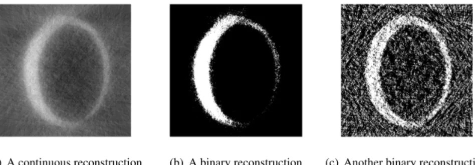
problem, but an approximation of it. When one is interested in finding a specific feature in binary tomography images, a specific reconstruction (either a solution or an approximate one) may not truly represent the original ground truth image. As an example, Figure 1.3 presents three different reconstructions of a ring-like shaped original image in which it is very difficult to determine, based on these reconstructions, whether the bottom right part of the ring is open.

(a) A continuous reconstruction (b) A binary reconstruction (c) Another binary reconstruction

Figure 1.3:Reconstructions of a ring-like shaped object using three different reconstruction

meth-ods. Is the “ring” open?

Even in cases when insufficient information is available to compute an accurate recon-struction of the complete image, it may still be possible to answer certain questions about the original image, or to determine certain features of it. Although finding a binary solution of the reconstruction problem is typically hard, it is often easier to prove that a solution with a specific featurecannotexist. For example, if the projections do not satisfy certain consistency conditions, a solution will certainly not exist.

When developing the error bounds for binary tomography, an existence condition for binary solutions of the reconstruction problem was found. In Chapter 8 we study the case where a pre-defined binary structure is enforced in the reconstruction problem and then a

consistencycondition for binary solutions is checked. By applying this methodology, it can be determined whether such a substructure can possibly occur, or whether it can certainly not occur in any binary image of the solution set.

1.5. Overview

As a conclusion of this introduction, we now provide a brief overview of the material con-tained in each of the next chapters.

InChapter 2, we derive a series of upper bounds that can be used to guarantee the quality

of a reconstructed binary image. The bounds limit the number of pixels that can be incorrect in the reconstructed image, in binary tomography, with respect to the original image. We provide several versions of these bounds, ranging from bounds on the difference between

(17)

approximate solutions and the original object.

In Chapter 3, we consider the problem of reconstructing a high-resolution binary image

from several low-resolution scans. Each of the pixels in a low-resolution scan yields the value of the sum of the pixels in a rectangular region of the high-resolution image. For any given set of such pixel sums, we derive an upper bound on the difference between a certain binary image which can be computed efficiently andanybinary image that corresponds with the given measurements. We also derive a bound on the difference between any two binary images having these pixel sums.

In Chapter 4 we expand the theory of error bounds for binary tomography of Chapter

2 to the case of noisy projection data. Despite the fact that the noiseless projection data is not available, we develop error bounds with respect to the solution set of the noiseless reconstruction problem.

InChapter 5we show how the error bounds of Chapter 2 can be adapted to be useful for

bounding the quality of experimental images. Our experimental results suggest that even though approximations have to be made due to noise and other errors in the data, the result-ing bounds can still provide guidance on estimatresult-ing the reconstruction quality in practice.

InChapter 6, we present a series of computable bounds that can be used with any projection

model. The approach developed in Chapter 2 is restricted to projection models where the corresponding matrix has constant column sums. We generalize these results and thereby broaden their applicability to include fan beam and cone beam projection models. In fact, the study presented here is not restricted to tomography and works for more general linear systems. We report the results of computational experiments for several phantom images, focused on parallel and fan beam projection models.

InChapter 7, we develop a discrete approximate reconstruction algorithm. Our algorithm

computes an image that has only grey values belonging to a given finite set. It also guar-antees that the difference between the given projections and the projections of the recon-structed discrete image is bounded. The bound, which is computable, is independent of the image size.

InChapter 8, we present a computational technique for discovering the possible presence of

(18)

Chapter 2

Bounds on the quality of

reconstructed images in binary

tomography

This chapter (with minor modifications) has been published as: K. J. Batenburg, W. For-tes, L. Hajdu, and R. Tijdeman. Bounds on the quality of reconstructed images in binary tomography. Discrete Applied Mathematics, Vol. 161(15), 2236–2251, 2013.

2.1. Introduction

Tomographyis a technique for reconstructing an image of an object from a series of pro-jections of this object, acquired from a range of viewing angles. The projection images are typically recorded using a scanning device, which can employ various types of beams (e.g., X-rays, neutrons, electrons) that traverse the object, after which a detector measures the res-ult of the beam-object interaction. Provided that a large number of high-quality projections are available, sampled from a full range of angles, an accurate reconstruction of the object can be computed using a tomographic reconstruction algorithm [25, 33].

In practice, the set of angles for which projections are acquired is often limited. Due to dose constraints, it can be desirable to record as few projection images as possible, while still attaining sufficient image quality. Also, the angular range can be restricted by the particular scanning setup, such as in electron tomography, where the shape of the sample holder limits the angular range of the projections [36]. The resulting image reconstruction problems, based on just a small number of projections, are known aslimited data problems.

For tomographic reconstruction from severely limited data, classical algorithms based on analytical inversion of the Radon transform, such as the Filtered Backprojection al-gorithm, often yield inferior reconstructions that are polluted by strong artefacts. In such cases, it makes sense to exploit available prior knowledge of the unknown object. Incorpor-ation of this knowledge in the reconstruction algorithm can potentially result in a reduction

(19)

of the required number of projections, increased accuracy of the reconstruction, or an im-proved ability to deal with noisy projection data. A prior that has received much attention recently concerns the sparsity of the image, or of its gradient, which is exploited in the field of Compressed Sensing [14, 16, 41, 42].

A related, but more strict type of prior knowledge is exploited inDiscrete Tomography, which focuses on the reconstruction of images that consist of a small, discrete set of grey values [27, 28]. The actual set of grey levels is typically assumed to be known in advance. Here, we focus specifically on the reconstruction ofbinaryimages, which consist of just two grey levels, 0 and 1. Several reconstruction algorithms have demonstrated the ability to reconstruct binary images from a very small number of projections, often even less than 6 [4, 6, 40].

Despite the strong constraint imposed on the grey values in discrete tomography, many valid solutions of the reconstruction problem can exist, all corresponding to the same set of projections. If the projections are obtained by performing measurements on some unknown ground truth object, the reconstruction can then deviate substantially from the true object.

As a consequence, there is a need for an upper bound on the difference between binary

solutions of the reconstruction problem. As the ground truth is a solution by itself, this would also yield a bound on the reconstruction error with respect to the ground truth.

A related problem in discrete tomography is the so-calledstability problem, which deals with the question how the reconstruction changes if the projections are slightly perturbed. For images represented on a discrete grid, both lower and upper bounds have been obtained for the magnitude of such changes [2–4, 46]. For the case of binary image reconstruction from just two projections, horizontal and vertical, bounds on the difference between binary images having the same projections have been obtained by Van Dalen [44, 45].

In this chapter, we present a series of bounds which are highly general. Our bounds can be computed for any set of projections and in different geometrical settings, for lattice images as well as discretized continuous images. A key idea in deriving these bounds is an observation first made by Hajdu and Tijdeman in [22], concerning the fact that all binary solutions of the reconstruction problem must lie on a certain hypersphere, of which both the center and radius can be computed. The center of this hypersphere, which we call the

central reconstruction, is the shortest real-valued solution of the tomography problem. This hypersphere construction leads directly to a simple bound on the distance between any two binary solutions, based on the triangle inequality. Stronger bounds can be derived by fo-cusing on the distance between binary solutions of the tomography problem and the binary

image that is obtained by roundingthe central reconstruction. We derive several bounds

that combine properties of the real-valued solution with combinatorial properties that are satisfied by the binary solutions. In particular, the fact that the sum of the pixel values in the unknown image is fully determined by the projection data can be used to improve the error bounds for binary images.

(20)

2.2. Notation and model 9

of the tomography problem. It is divided in three parts: in Section 2.4.1, a general bound is derived on the difference between two binary images having a given set of projections. Section 2.4.2 deals with bounds that are based on properties of the binary images that are obtained by rounding the central reconstruction. These bounds are subsequently refined in Section 2.4.3 by including the knowledge of the total number of 1’s in any binary solution, which can be determined from the projection data.

Section 2.5 presents a series of simulation experiments and their results. From these results, the practical value of the proposed bounds can be evaluated for different types of images. The results are further discussed in Section 2.6. Section 2.7 concludes the chapter.

2.2. Notation and model

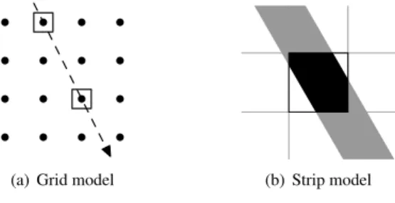
Throughout the discrete tomography literature, several imaging models have been

con-sidered. In the grid model, an image is formed by assigning a value to each point in a

regular grid. In the case of binary images, each point is assigned a value of either 0 or 1. Here, we consider square grids of the form A={(i,j)∈_Z2_{: 1}_≤_i_,_j_≤_s_}_for _s_∈

N,s≥1; see Fig. 2.1(a). For the grid model, we refer to the points inAas pixels. A binary image defined onAcan be represented by a mapA→ {0,1}. Aprojectionof an image f is formed by considering the set of parallel lines through one or more grid points in a certain direction (a,b)∈_Z2, witha≥0 and (a,b) coprime, and summing the values of the points on each line. For a line given by the equationax−by=t(t∈_Z), theline projection pis defined as

p= X

(x,y)∈A:ax−by=t

f(x,y).

The grid model can be used to model nanocrystals, that consist of discrete atoms positioned in a regular grid [1, 31].

(a) Grid model (b) Strip model

Figure 2.1:Two different projection models.

In many tomography applications, a continuousrepresentation of the object is more

(21)

strips in a given direction and for each strip computing the weighted sum of all the pixels which intersect that strip with a weight equal to the intersection area of the strip and the pixel.

We now define some general notation. Animageis represented by a vectorx=(xi)∈Rn. We refer to the entries of xaspixels, which correspond to unit squares in the strip model and to points in the grid model. The derivation of our main results does not depend on the particular projection model. Throughout this chapter we assume that all images are square, consisting ofcrows andccolumns, wheren=c2_{. A}_{binary image}_{corresponds with a vector}

¯

x∈ {0,1}n_.

For a given set ofkprojection directions, theprojection mapmaps an imagexto a vector

p∈_Rmofprojection data, wheremdenotes the total number of line measurements. As the projection map is a linear transformation, it can be represented by a matrixW=(wi j)∈Rm×n, called the projection matrix. Entry wi j represents the weight of the contribution ofxj to

projected linei. Note that for the grid model the projection matrix is a binary matrix, while for the strip model its entries are real values in [0,1]. The projection matrixWand vector p

can be decomposed intokblocks as

W=             W1 .. . Wk            

, p=

            p1 .. . pk             , (2.1)

where each blockWd(d=1,...,k) represents the projection map for a single direction and each block pdrepresents the corresponding projection data.

From this point on, we assume that the projection matrix has the property that Pm

i=1wi j=kfor all j=1,...,n. This property is certainly satisfied for the grid model, as

every xj is counted with weight 1 for exactly one line in each projection direction. The

property is also satisfied for the strip projection model, as the total pixel weight for each projection angle is equal to the area of a pixel, which is 1. For most other projection models commonly used in tomography, such as the line model, where the weight of a pixel is de-termined by the length of its intersection with a line, this property is approximately satisfied, but not always exactly.

Thegeneral reconstruction problemconsists of finding a solution of the systemW x=p

for given projection data p, i.e., to find an image that has the given projections. Inbinary tomography, one seeks a binary solution of the system. For a given projection matrixWand given projection data p, letSW(p)={x∈Rn:W x=p}, the set of all real-valued solutions corresponding with the projection data, and let ¯SW(p)=SW(p)∩ {0,1}n, the set of binary

solutionsof the system. As the main goal of incorporating prior knowledge of the binary grey levels in the reconstruction is to reduce the number of required projections, we focus on the case wheremis small with respect ton, such that the real-valued reconstruction problem is severely underdetermined.

Despite the strong constraint that each pixel valuexi must belong to the set{0,1}, the

(22)

2.3. The central reconstruction 11

thatanysuch solution must be close to the original object from which the projections have been obtained, even if the exact set of differences cannot be determined.

For any two vectors ¯u,v¯∈ {0,1}n, define thedifference setD( ¯u,v¯)={i: ¯ui,v¯i}and the

number of differencesd( ¯u,¯v)=#D( ¯u,v¯), where the symbol # denotes the cardinality operator for a finite set. Note that d( ¯u,v¯)=ku¯−vk¯ 1.

2.3. The central reconstruction

As the projection matrix is typically not a square matrix, and also does not have full rank, it does not have an inverse. Recall that theMoore-Penrose pseudo inverseof anm×nmatrixA

is ann×mmatrixA†, which can be uniquely characterized by the two geometric conditions

A†b⊥ N(A) and (I−A A†)b⊥ R(A) for all b∈_Rm,

whereN(A) is the nullspace ofAandR(A) is the range ofA, [12, page 15].

Letx∗=W†p. Thenx∗has the property (see Chapter 3 of [11]) that it is the real-valued solution of minimal Euclidean norm of the systemW x=p, provided that the latter system is solvable. We callx∗thecentral reconstructionof p. The central reconstruction plays an important role in the bounds we derive for the binary reconstruction problem. We will show in the next section that all binary solutions of the system have equal distance tox∗, so that one can consider the central reconstruction as lying “in the middle” of all binary solutions.

As all bounds presented in this chapter depend on x∗_{, accurate computation of} _x∗ _is

necessary to compute the corresponding difference bounds. One approach to computing

the central reconstruction of a consistent systemW x=pis to use the QR decomposition ofWT_{. We will only sketch the computation here and refer to [5] for details. For clarity of}

presentation, we assume thatWhas full row rank. In fact, this assumption is not satisfied for

tomography, and theextended QR decomposition should be used. The QR decomposition

factorizes the matrixWT _{into an orthogonal matrix}_Q_{and an uppertriangular matrix}_R_of

full column rank, as

WT =Q R

0

! .

The central reconstruction is then given by x∗=Q(RT)−1p, which can be computed effi -ciently by first solving the systemRTy=pforyby back substitution, and then computing

x∗=Qy.

However, due to the size of the matrixW, calculation of the QR decomposition is usually unpractical for large images. For the casem<n, the QR decomposition requiresO(n3) oper-ations. Moreover, then×nmatrixQis typically dense, requiring a vast amount of computer memory. As an alternative, an iterative method for solving the systemW x=p, calledCGLS

(Conjugate Gradient Least Squares), can be used [39]. The CGLS algorithm can effectively exploit the sparse structure of the projection matrix to reduce the required computation time, and does not require storage of large, dense matrices. Apart from numerical errors, applying CGLS to the systemW x=presults, after convergence, in the computation ofW†_p_{, while}

not computing the matrixW†_{explicitly (see also [47]). For all experiments in Section 2.5,}

(23)

2.4. Quality bounds for binary solutions

In all the results in the following subsections, we consider a fixed systemW x=p corres-ponding to a binary tomography problem, and refer to the central reconstruction of this system asx∗.

As a substantial number of bounds will be given throughout this chapter, we introduce the following notation that will be further defined in the remainder of the chapter:

• The expressionsa(i) (i=1,2,3,4) will represent bounds on the number of pixel dif-ferences between any two binary solutions of the reconstruction problem.

• The expressionsb(i) (i=1,2,3,4) will represent bounds on the number of pixel diff er-ence between a certain given binary image (not necessarily a solution) and any binary solution of the reconstruction problem.

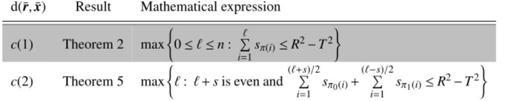
• The expressionsc(i) (i=1,2) will represent bounds on the number of pixel differences between therounded central reconstruction¯rand any binary solution.

The bounds within each class a,b, andc represent upper bounds for the same distance

measure and can therefore be compared.

2.4.1. Elementary bounds based on the central reconstruction

In this subsection, a first set of bounds are derived. They follow from the fact that the Eu-clidean distance between the central reconstruction and any binary solution of the recon-struction problem can be determined from the projections. We start by noticing that the Euclidean norm of any binary solution of the tomography problem is determined by the projection data:

Lemma 1. Letx¯∈S¯W(p). Then,kxk¯ 2₂=kp_kk1.

Proof. By the definition of the`1-norm,kpk1=Pmi=1|pi|=Pmi=1pi, sincepi≥0 (i=1,...,n).

Also,

m

X

i=1

pi= m

X

i=1

         n X

j=1

wi jx¯j

         = n X

j=1

        m X

i=1

wi j

        ¯

xj= n

X

j=1

kx¯j, (2.2)

and thereforekpk1=kPn_j₌₁x¯j.

As ¯x∈ {0,1}n_{, we have}_k_xk_¯ 2

2=kxk¯ 1=

Pn j=1x¯j=

kpk1

k .

The following lemma illustrates the importance of the central reconstruction, the shortest real-valued solution inSW(p), by showing that the binary solutions are the shortest among all integer solutions of the system.

Lemma 2. Letx¯∈S¯W(p)andy∈SW(p)∩Zn. Thenkxk¯ 2≤ kyk2, with equality if and only

(24)

2.4. Quality bounds for binary solutions 13

Proof. Note that the statement is proved in [22], see Problem 2 and the subsequent para-graph. However, for the convenience of the reader we give the proof here.

We have

||x||¯ 2₂=

n

X

i=1

¯

x2_i =

n

X

i=1

¯

xi= n

X

i=1

yi=

kpk1

k . (2.3)

Observing that

n

X

i=1

yi≤ n

X

i=1

y2_i =||y||2₂, (2.4)

with equality if and only ifyis binary, yields the result.

Lemma 3. Letx¯∈S¯W(p). Thenkx¯−x∗k2=

q

kpk₁

k − kx

∗_k2 2.

Proof. From the definition of x∗ we have ( ¯x−x∗)∈ N(W), andx∗⊥( ¯x−x∗). Applying Pythagoras’ Theorem and Lemma 1 yields

kx¯−x∗k2

2=

kpk1

k − kx

∗_k2

2. (2.5)

DefineR=

q

kpk1

k − kx∗k22. We will use this constant throughout the remainder of this

chapter, and refer toRas thecentral radius. According to Lemma 3, any binary solution of the reconstruction problem is on the hypersphere centered inx∗with radiusR.

Supposing the existence of at least two different binary solutions, Lemma 3 allows us to derive an upper bound for the number of pixel differences between those solutions.

Theorem 1. Letx¯,¯y∈S¯W(p)and put a(1)=4R2. Thend( ¯x,y¯)≤a(1).

Proof. According to Lemma 3, we havekx¯−x∗k₂=ky¯−x∗k₂=R. Therefore,

kx¯−yk¯ 2≤ kx¯−x∗k2+ky¯−x∗k2=2R.

As ¯xand ¯yare binary, we have d( ¯x,y¯)=kx¯−yk¯ 1=kx¯−yk¯ 2₂.

Using the triangle inequality, a simple bound can also be given for the distance between

anybinary image and a solution of the reconstruction problem, as follows:

Corollary 1. Letv¯∈ {0,1}n_{be a given binary image and put b}₍₁₎₌₍_R₊_k_v_¯₋_x∗_k

2)2. Then

(25)

2.4.2. Bounds based on rounding the central reconstruction

The fact that all elements of ¯SW(p) have equal distance to the central reconstruction x∗, combined with the facts that binary solutions are the shortest solutions among all integer solutions (Lemma 2) and that x∗ is the shortest real-valued solution, suggests that binary solutions can often be found near x∗_{. It is therefore natural to consider the image that is}

obtained by rounding each entry of x∗_{to the nearest binary value. In this section, we will}

derive several bounds based on the number of differences between a binary solution of the reconstruction problem and a binary image obtained by roundingx∗_.

Forα∈_R, let bin(α)=min(|α|,|1−α|). PutT=

q Pn

i=1bin 2₍_x∗

i), i.e., the Euclidean

dis-tance fromx∗to the nearest binary vector. We will use this constant throughout this chapter and refer toT as thecentral rounding distance.

Corollary 2. If R<T , thenS¯W(p)=∅.

If R=T , then all solutions inS¯W(p)can be obtained by rounding the values inx∗to the

nearest binary values, and variations are only possible for the entries i where x∗_i =1₂.

LetT ={v¯∈ {0,1}n_: _k_v−_¯ _x∗_k

2=T}and let ¯r∈ T, i.e., ¯ris among the binary vectors that

are nearest tox∗_{in the Euclidean sense.}

IfR>T andR−T is small, it is possible to say that a fraction of the rounded values are correct, i.e., to provide an upper bound on thenumberof pixel differences between any solution in ¯SW(p) and ¯r. In most cases we can not saywhichrounded values are correct.

Lemma 4. Letr¯∈ T and letv¯∈ {0,1}nbe any binary vector.

Thenkv¯−x∗_k2

2=T

2₊P

i∈D(¯v,¯r)|2x∗i−1|.

Proof. We have the following identities:

kv¯−x∗k2

2 = kv¯−¯r+r¯−x ∗_k2

2

= k¯r−x∗k2

2+2h¯r−x ∗_,

¯

v−¯ri+hv¯−r¯,v−¯ ¯ri

= T2+2h¯r−v¯,x∗i+kvk¯ 2₂− k¯rk2₂

= T2+2

n

X

i=1

(¯ri−v¯i)x∗i+ n

X

i=1

¯

vi− n

X

i=1

¯

ri

= T2+

n

X

i=1

(¯ri−v¯i)(2x∗i−1)

= T2+ X

i∈D(¯v,¯r)

|2x∗_i −1|.

Lemma 4 can be interpreted as follows: consider the set of entries where ¯rand ¯vare different. If we transform ¯rinto ¯vby performing a sequence of single-entry changes (either from 0 to 1, or from 1 to 0), each time an entryi of ¯ris changed the squared Euclidean distance from the current vector tox∗_{increases by}_s

i=|2x∗_i−1|.

Letπbe a permutation of {1,...,n} such that sπ(1)≤sπ(2)≤...≤sπ(n), which can be

(26)

2.4. Quality bounds for binary solutions 15

Corollary 3. Letr¯∈ T and letv¯∈ {0,1}nbe any binary vector. Then

kv−¯ x∗k2 2≥T

2₊

` X

i=1

sπ(i),

where`=d(¯r,v¯).

Proof. According to Lemma 4 we have

kv¯−x∗k2₂=T2+ X

i∈D(¯r,v¯)

si≥T2+

` X

i=1

sπ(i).

As the Euclidean distance fromx∗_{to any ¯}_x_∈_S_¯

W(p) isR, a bound can now be derived on the maximal number of pixels in ¯rthat must be changed to move from ¯rto ¯x.

Theorem 2. Let¯r∈ T,x¯∈S¯W(p). Put

c(1)=max       

0≤`≤n: ` X

i=1

sπ(i)≤R2−T2

       .

Thend( ¯x,¯r)≤c(1).

Proof. As ¯x∈S¯W(p), we havekx¯−x∗k2₂=R2.Applying Lemma 4, we find that

R2−T2= X

i∈D( ¯x,¯r)

si≥ d( ¯x,r¯)

X

i=1

sπ(i),

which implies that d( ¯x,r¯)≤c(1).

The proof of Theorem 2 can be interpreted as follows: consider the set of entries where ¯

rand ¯xare different. If we transform ¯rinto ¯x by performing a sequence of single-entry changes (either from 0 to 1, or from 1 to 0), each time an entryiof ¯ris changed the squared Euclidean distance from the current vector to x∗_{increases by} _s

i=|2x∗_i−1|. As all binary

solutions of the reconstruction problem are on a hypersphere centered inx∗_{with radius}_R_,

we know that once we have crossed the boundary of this hypersphere, a binary solution can no longer be obtained by changing the values of additional entries that have not yet been changed. An upper bound on the number of differences between ¯rand ¯xcan be obtained by counting the number of steps required to cross the hypersphere, each time choosing a pixel which results in the minimal increase of the distance tox∗. The following two Corollaries follow directly from Theorem 2:

Corollary 4. Let ¯r∈ T,x¯,y¯∈S¯W(p)and let a(2)=2c(1)with c(1)defined as in Theorem

2. Thend( ¯x,¯y)≤a(2).

Corollary 5. Let¯r∈ T and letv¯∈ {0,1}n_{be a given binary image and let b}₍₂₎₌_c₍₁₎₊_d(¯_r_,_v_¯₎

(27)

In fact, the bound from Corollary 4 can be sharpened by noting that we can assume that the sets D(¯r,x¯) and D(¯r,y¯) are disjoint, as entries that occur in both sets do not contrib-ute to the number of differences between ¯xand ¯y. This observation leads to the following Theorem:

Theorem 3. Let¯r∈ T,x¯,y¯∈S¯W(p). Put

a(3)=max       

0≤`≤n: ` X

i=1

sπ(i)≤2(R2−T2)

       .

Thend( ¯x,¯y)≤a(3).

Proof. Define ˆx by ˆxi=r¯i if ¯xi=y¯i, and ˆxi=x¯i otherwise. Define ˆyanalogously. Then

d( ˆx,yˆ)=d( ¯x,¯y),kxˆ−x∗k2

2≤R

2_{, and}_k_y_ˆ₋_y∗_k2

2≤R

2_{. Hence,}

2R2≥ kxˆ−x∗k2₂+kˆy−y∗k2₂=2T2+ X

i∈D(¯r,xˆ)

si+

X

i∈D(¯r,yˆ)

si.

AsD(¯r,xˆ) andD(¯r,yˆ) are disjoint, we have 2R2−2T2≥Pd(¯r,xˆ)+d(¯r,yˆ)

i=1 sπ(i).This implies that

d( ¯x,y¯)=d( ˆx,ˆy)≤d(¯r,xˆ)+d(¯r,yˆ)≤a(3).

A similar bound can be derived for the case where a particular binary image ¯v, not necessarily a solution of the tomography problem, is given. For this, we transform ¯vinto ¯r

and then we perform a sequence of single-entry changes in ¯rwith the exclusion of the pixels that differ between ¯vand ¯rbecause they have already been counted as wrong pixels of ¯v.

Theorem 4. Let¯r∈ T and letv¯∈ {0,1}nbe a given binary image. Consider the sequence

(φ(1),φ(2),...,φ(˜n))defined by removing all numbers i for whichv¯i,r¯ifrom the sequence

(π(1),...,π(n)). Put

U=max       

0≤`≤n˜: ` X

i=1

sφ(i)≤R2−T2

      

and let b(3)=U+d(¯r,v¯). Then for any binary imagex¯∈S¯W(p), we haved( ¯x,v¯)≤b(3).

Proof. Define ˆxby ˆxi=r¯iif ¯xi=v¯i, and ˆxi=x¯iotherwise. Similarly, define ˆvby ˆvi=r¯iif

¯

xi=v¯i, and ˆvi=v¯i otherwise. Then d( ˆx,vˆ)=d( ¯x,v¯), d(ˆv,¯r)≤d(¯v,¯r), andkxˆ−x∗k2₂≤R2.

Hence, R2_{≥ k}_x_ˆ₋_x∗_k2

2=T2+

P

i∈D(¯r,xˆ)si. As D(¯r,xˆ) and D(¯r,v¯) are disjoint, we have

R2−T2≥Pd(¯r,xˆ)

i=1 sφ(i).This implies that d( ¯x,v¯)=d( ˆx,vˆ)≤d( ˆx,¯r)+d(¯r,vˆ)≤U+d(¯r,v¯).

2.4.3. Bounds involving the number of ones in binary solutions

The fact that the`1-normkxk¯ 1of any binary solution is determined by the projection data,

(28)

2.5. Experiments and results 17

For any two vectors ¯u,v¯∈ {0,1}n, define the sets D0( ¯u,v¯)={i: ¯ui=0∧v¯i=1} and

D1( ¯u,v¯)={i: ¯ui=1∧v¯i=0}. We also define d0( ¯u,v¯)=#D0( ¯u,v¯) and d1( ¯u,v¯)=#D1( ¯u,v¯).

Ifkxk¯ 1=k¯rk1, we have d0(¯r,x¯)=d1(¯r,x¯)=d(¯r,x¯)/2. In other words, in order to

trans-form ¯r into ¯x, the number of pixels of ¯r assigned to 0 that must be changed to 1 is equal to the number of pixels of ¯r assigned to 1 that must be changed to 0. In general, when kxk¯ 1=krk¯ 1is not necessarily true, lett=kxk¯ 1− k¯rk1. Hence, d0(¯r,x¯)=d1(¯r,x¯)+t,

which gives d0(¯r,x¯)−t/2=d1(¯r,x¯)+t/2=d(¯r,x¯)/2. Therefore, d0(¯r,x¯)=d(¯r,x¯)/2+t/2

and d1(¯r,x¯)=d(¯r,x¯)/2−t/2.

Theorem 5. Let¯r∈ T and t=kxk¯ 1− k¯rk1. Construct the sequence(π0(1),π0(2),...,π0(n0))

by removing all numbers i for which ¯ri=1 from the sequence(π(1),...,π(n)). Similarly,

construct the sequence(π1(1),π1(2),...,π1(n1))by removing all numbers i for whichr¯i=0

from the sequence(π(1),...,π(n)). Let

c(2)=max         

`: `+tis even and

min((`+t)/2,n0)

X

i=1

sπ0(i)+

min((`−t)/2,n1)

X

i=1

sπ1(i)≤R 2₋_T2

         .

Then for any binary imagex¯∈S¯W(p), we haved(¯r,x¯)≤c(2).

Proof. Let ¯x∈S¯W(p).Put ˜`=d(¯r,x¯). Then

R2−T2= X

i∈D(¯r,x¯)

si=

X

i∈D0(¯r,x¯)

si+

X

i∈D1(¯r,x¯)

si≥ ( ˜`+t)/2

X

i=1

sπ0(i)+ ( ˜`−t)/2

X

i=1

sπ1(i)

with ( ˜`+t)/2≤n0and ( ˜`−t)/2≤n1, which implies that ˜`=d(¯r,x¯)≤c(2).

Corollary 6. Let c(2)be as defined in Theorem 5 and define a(4)=2c(2). Then for any pair

of binary imagesx¯,¯y∈S¯W(p), we haved( ¯x,y¯)≤a(4).

Corollary 7. Letv¯∈ {0,1}n_{be a given binary image and let b}₍₄₎₌_c₍₂₎₊_d(¯_r_,_v_¯₎_{with c}₍₂₎

as defined in Theorem 5. Then for any binary imagex¯∈S¯W(p), we haved(¯v,x¯)≤b(4).

2.5. Experiments and results

A series of experiments have been performed to investigate the practical value of the bounds given in the several theorems and corollaries presented, for a range of images. The experi-ments are all based on simulated projection data obtained by computing the projections of the test images (so-calledphantoms) in Fig. 2.2:

Phantom 1represents a very simple, convex shaped object.

Phantom 2represents an object with a more complex boundary. Also, the object is not

convex and the boundary is fairly complex.

Phantom 3represents a cross-section of a cylinder head in a combustion engine. It

(29)

(a) Phantom 1 (b) Phantom 2 (c) Phantom 3 (d) Phantom 4

Figure 2.2:Original phantom images used for the experiments.

Phantom 4was constructed from a micro-CT image of a rat bone, acquired with a SkyScan

1072 cone-beam micro-CT scanner.

All phantom images have a size of 512×512 pixels. To perform images with varying image size (smaller than 512×512), the phantoms have been downscaled to obtain binary images of the appropriate sizes.

In each experiment, the central reconstruction x∗ was first computed using the CGLS algorithm. For some of the bounds, it is necessary to compute the rounded central recon-struction ¯rwhich was performed by roundingx∗to the nearest binary vector, choosing ¯ri=1

if x∗_i =1₂. Based on x∗ _{and ¯}_r_{, the various upper bounds described in Sections 2.4.1–2.4.3}

were computed.

When presenting the results, we express the bounds on the pixel differences between two images as afractionof the total number of image pixels. This allows for more straight-forward interpretation of the results than using the absolute number of pixel differences. To aid in the identification of the bounds, Tables 2.1–2.3 provide a summary of all bounds and their respective theorems/corollaries.

d( ¯x,y¯) Result Mathematical expression

a(1) Theorem 1 4R2

a(2) Corollary 4 2 max

(

0≤`≤n: P`

i=1

sπ(i)≤R2−T2 )

a(3) Theorem 3 max

(

0≤`≤n: P`

i=1

sπ(i)≤2(R2−T2) )

a(4) Corollary 6 2 max

(

`: `+sis even and

(`+s)/2 P i=1

sπ0(i)+

(`−s)/2 P i=1

sπ1(i)≤R

2₋_T2 )

Table 2.1: List of symbolic expressions used for the bounds on the number of pixel differences

(30)

d(¯v,x¯) Result Mathematical expression

b(1) Corollary 1 (R+kv¯−x∗_k

2)2

b(2) Corollary 5 max

(

0≤`≤n: P`

i=1

sπ(i)≤R2−T2 )

+d(¯r,v¯)

b(3) Theorem 4 max

(

0≤`≤n:

` P i=1

sφ(i)≤R2−T2 )

+d(¯r,¯v)

b(4) Corollary 7 max

(

`: `+sis even and

(`+s)/2 P i=1

sπ0(i)+

(`−s)/2 P i=1

sπ1(i)≤R

2₋_T2 )

+d(¯r,¯v)

between a given¯v∈ {0,1}n_{and any binary solution, their respective theorems}_/_{corollaries and}

math-ematical expressions.

d(¯r,x¯) Result Mathematical expression

c(1) Theorem 2 max

(

0≤`≤n: ` P

i=1

sπ(i)≤R2−T2

)

c(2) Theorem 5 max

(

`: `+sis even and

(`+s)/2

P

i=1 sπ0(i)+

(`−s)/2

P

i=1

sπ1(i)≤R

2₋_T2

)

between ¯rand any binary solution, their respective theorems/corollaries and mathematical expres-sions.

All graphs presented in the following subsections use a logarithmic scale for the error bounds. In some cases, the bound may become very small, or even 0, resulting in a point on the graph that cannot be plotted. These points are simply removed from the plot, causing the graph to be disconnected.

The remainder of this section is structured as follows. First, the concepts of central re-construction, central radius, and rounded central reconstruction are illustrated for a concrete example in Section 2.5.1. Next, experimental results for the grid model and the strip model are presented in Sections 2.5.2 and 2.5.3, respectively. In Section 2.5.4, we consider a scen-ario where a binary reconstruction has been computed by a certain reconstruction algorithm, and we are interested in bounding the error with respect to the phantom for this particular reconstruction.

2.5.1. Concepts and interpretation

Fig. 2.3(a) shows the central reconstructionx∗_{of size 128}_×_{128, based on}_k₌_{4 projections}

(31)

using the grid model for the directions{(0,1),(1,0),(1,1),(1,−1)}. The central reconstruc-tion was computed using the CGLS algorithm, as explained in Secreconstruc-tion 2.3. The difference between the phantom image and the central reconstruction is shown in Fig. 2.3(b), where the grey levels are scaled between−1 (black) and 1 (white). Note that this difference vec-tor ¯x−x∗_{is in the nullspace of}_W_{, as ¯}_x_and_x∗ _{are both solutions of the system}_{W x}₌_p_.

Therefore, the difference image can be considered as aswitching componentin the sense that it can be added to any other image without changing the projections in the four chosen directions.

Thecentral radius Rcorresponds to the Euclidean norm of the difference vector ¯x−x∗, which is around 31.3152 in this case. Fig. 2.3(c) shows the rounded central reconstruction ¯

r, which is formed by rounding each pixel of x∗ to the nearest binary value. Thecentral rounding distance Tcorresponds with the Euclidean norm of the difference ¯r−x∗, which is around 25.5704 in this case. Note that ¯ris usuallynota solution of the systemW x=p. The difference between the phantom ¯xand the image ¯ris shown in Fig. 2.3(d). This difference image is a three-valued image, with pixel values from the set{−1,0,1}. The bounds from Section 2.4.2 and onwards are based on bounding the norm of this difference image.

Similar images for the case ofk=16 projections are shown in Fig. 2.3e-h, based on the direction set{(1,0),(0,1),(1,1),(1,−1),(1,2),(1,−2),(2,1),(2,−1),(1,3),(1,−3),(2,3), (2,−3),(3,1),(3,−1),(3,2),(3,−2)}. It can be clearly observed that, as the number of pro-jections increases, the central reconstruction and the rounded central reconstruction both become better approximations of the phantom image. For the case of 16 projections, the difference between ¯xand ¯ris already surprisingly small (approximately 0.45% of the total number of pixels), even though the systemW x=pis highly underdetermined.

(a) k=4 :x∗ _(b)_k₌_{4 : ¯}_x₋_x∗ _(c)_k₌_{4 : ¯}_r _(d)_k₌_{4 : ¯}_x₋_¯_r

(e) k=16 :x∗ _(f)

k=16 : ¯x−x∗ _(g)

k=16 : ¯r (h)k=16 : ¯x−¯r

(32)

2.5.2. Error bounds for the grid model

In the grid model, a projection direction is represented by a pair of integers (a,b)∈_Z2_,

such that gcd(a,b)=1 anda≥0. LetAbe the set of all such pairs. For any positive in-teger c, put A_c:={(a,b)∈ A: max(a,|b|)=c}and order the elements of A_c, firstly by increasing value ofa, secondly by increasing value of|b|, and thirdly by decreasing value of b. For example, A₃={(1,3),(1,−3),(2,3),(2,−3),(3,1),(3,−1),(3,2),(3,−2)}. For any positive integerc, the ordered setD_cis formed by concatenatingA₁,...,A_c; for example,

D₃={(0,1),(1,0),(1,1),(1,−1),(1,2),(1,−2),(2,1),(2,−1),(1,3),(1,−3),(2,3),(2,−3), (3,1),(3,−1),(3,2),(3,−2)}. To perform an experiment withkprojection angles, the firstk

directions were selected from the setD₂₀. This means that when the number of directions is increased, the old set of directions is always included in the new set of directions.

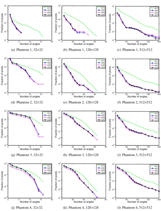
Experiments have been performed based on the three phantom images, scaled to sizes of 32×32, 128×128 and 512×512 respectively, varying the number of projection directions. The maximum number of projection directions for each image size is of 16, 64 and 200, respectively.

The first set of results are shown in Fig. 2.6, where bounds on the distance between any two binary solutions of the reconstruction problem, bounds on the number of differences between ¯rand the phantom image ¯x, and the exact error between ¯rand the phantom image

¯

x are jointly plotted. The bounds a andcwere obtained by computing the minimum of

all bounds in Tables 2.1 and 2.3 for each test case, i.e.,a=min{a(1),a(2),a(3),a(4)}and

c=min{c(1),c(2),c(3),c(4)}. In Fig. 2.7, the individual boundsa(1)–a(4) are shown for the same experiments.

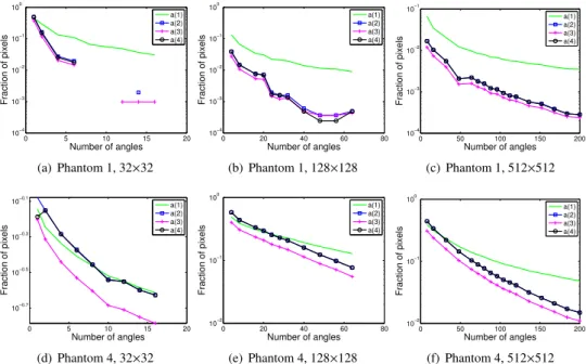
2.5.3. Error bounds for the strip model

The experiments for the strip model have been performed using projection angles selec-ted to coincide with the projection directions specified for the grid model. The projection angles were selected in this way to make the two models comparable. Projections have been computed based on sets of parallel strips, each strip having a width that equals the pixel size.

Experiments have been performed based on the four phantom images, scaled to sizes of 32×32, 128×128 and 512×512 respectively, varying the number of projection directions. The maximum number of projection directions for each image size is of 16, 64 and 200, respectively.

For the sake of compactness, we include the results for Phantoms 1 and 4. We did not observe strong deviations in the general behaviour of the bounds for the two other phantoms. The first set of results are shown in Fig. 2.8, where bounds on the distance between any two binary solutions of the reconstruction problem, bounds on the number of differences between ¯rand the phantom image ¯x, and the exact error between ¯rand the phantom image

¯

x are jointly plotted. The bounds a andcwere obtained by computing the minimum of

all bounds in Tables 2.1 and 2.3 for each test case, i.e.,a=min{a(1),a(2),a(3),a(4)}and

(33)

2.5.4. Error bounds for a particular reconstruction

So far, the experiments were focused on bounding the difference between any two binary solutions, or the difference between ¯rand any binary solution. In practice, it can also be important to know bounds on the difference between any binary solution and aparticular

binary image, computed by a certain reconstruction algorithm. As the problem of computing a binary solution of the reconstruction problem is usually very hard, we will not assume that such a binary reconstruction is an exact solution to the reconstruction problem.

Several algorithms have been proposed in the literature for reconstructing binary im-ages from their projections, see, e.g., [6, 9, 28, 40]. As an example, we focus here on the Discrete Algebraic Reconstruction Technique (DART), which has recently been proposed as a promising reconstruction algorithm for discrete tomography [7, 9]. The binary recon-struction computed by DART is not guaranteed to be an exact solution of the tomography problem.

(a)k=4 (b)k=6 (c)k=8 (d)k=10

Figure 2.4:DART reconstructions of Phantom 3 from 4, 6, 8 and 10 projections.

DART reconstructions have been computed for Phantoms 1, 2 and 3, using the strip model with projection angles equally distributed between 0 and 180 degrees. As an illus-tration of the reconstruction results, Fig. 2.4 shows reconstructions of Phantom 3 for an increasing number of projections.

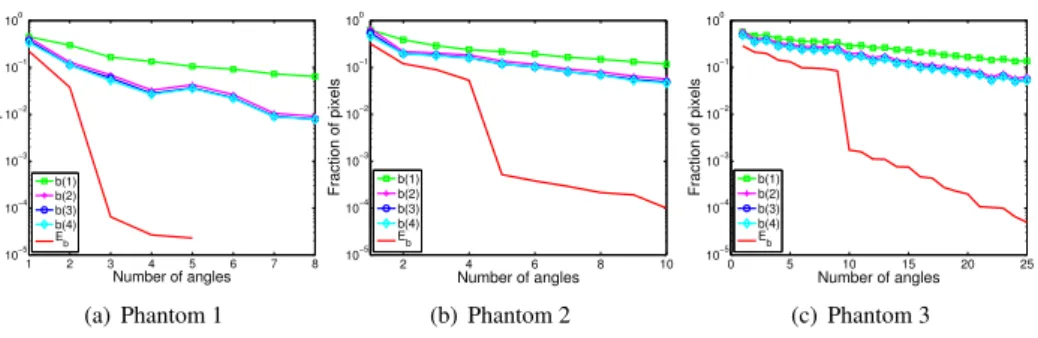
The boundsb(1),...,b(4) were computed, which bound the fraction of different pixels between the DART reconstruction and the original phantom. The results are shown in Fig. 2.5. The figure also contains graphs for the actual fraction of pixel differencesEbbetween

the DART reconstruction ¯vand the phantom.

(34)

2.6. Discussion of the results 23

1 2 3 4 5 6 7 8

10−5 10−4

10−3

10−2

10−1

100

Number of angles Fraction of pixels b(1)_b(2)

b(3) b(4) E_b

(a) Phantom 1

2 4 6 8 10

10−5 10−4 10−3 10−2 10−1 100

Number of angles Fraction of pixels b(1)b(2)

b(3) b(4) E_b

(b) Phantom 2

0 5 10 15 20 25

10−5 10−4 10−3 10−2 10−1 100

Number of angles Fraction of pixels b(1)b(2)

b(3) b(4) E_b

(c) Phantom 3

Figure 2.5:Error bounds for DART reconstruction of the three phantoms (size512×512) as function

the number of projection angles. Note that the graphs for b(2), b(3), and b(4)have strong overlap and can hardly be distinguished.

2.6. Discussion of the results

Despite the facts that the four phantoms have strong differences in shape and morphology, and that the grid and strip models are quite different, the results shown in Figs. 2.6–2.9 are surprisingly consistent throughout all experiments. Most of the bounds become smaller as the number of projection directions is increased but monotonicity is not a property of all the bounds presented in Section 2.4.

From the difference between the bounds presented in Section 2.4.1 and the bounds based on the rounded central reconstruction, we see that in most cases the phantom ¯xis substan-tially closer to ¯rthan tox∗.

In Figs. 2.6 and 2.8, it can be observed that the true fraction of pixel differences between the phantom image ¯x and the rounded central reconstruction ¯r, denoted byEc, is often

approximated quite well by the boundc, in particular for the grid model. This indicates that with respect to ¯r, the bounds presented in this chapter can be quite sharp.

In Fig. 2.8(a), parts of the graphs for the boundsaandc, for more than 6 projections, are missing. In fact, in this case all of them are zero, such that they cannot be displayed in the logarithmic scale. This illustrates that our theorems for bounding the distance between any two binary solutions can be used to prove uniqueness of a binary solution, even when the corresponding real-valued system of equations is underdetermined.

(35)

2.7. Outlook and conclusions

In this chapter, we have presented a range of general bounds on the accuracy of recon-structions in binary tomography, with respect to the unknown original object. The bounds can be computed within reasonable time and give guarantees on the number of pixels that can be different between any two binary solutions of the tomography problem, on the dif-ference between an image obtained by rounding the central reconstruction and any binary

solution, and on the difference betweenany binary image and any binary solution. The

(36)

2.7. Outlook and conclusions 25

1 2 3 4 5 6 7

10−3 10−2 10−1 100

Number of angles

Fraction of pixels

a c E

c

(a) Phantom 1, 32×32

0 5 10 15 20 25 30

10−4 10−3 10−2 10−1

Number of angles

Fraction of pixels

a c E_c

(b) Phantom 1, 128×128

0 50 100 150 200

10−6 10−5 10−4 10−3 10−2 10−1

Number of angles

Fraction of pixels

a c E_c

(c) Phantom 1, 512×512

0 2 4 6 8 10 12

10−3 10−2 10−1 100

Number of angles

Fraction of pixels

a c E_c

(d) Phantom 2, 32×32

0 10 20 30 40 50 60

10−4 10−3 10−2 10−1 100

Number of angles

Fraction of pixels

a c E_c

(e) Phantom 2, 128×128

0 50 100 150 200

10−5 10−4 10−3 10−2 10−1

Number of angles

Fraction of pixels

a c E_c

(f) Phantom 2, 512×512

0 5 10 15

10−3 10−2 10−1 100

Number of angles

Fraction of pixels

a c E_c

(g) Phantom 3, 32×32

0 10 20 30 40 50 60

10−4 10−3 10−2 10−1 100

Number of angles

Fraction of pixels

a c E_c

(h) Phantom 3, 128×128

0 50 100 150 200

10−6 10−4 10−2 100

Number of angles

Fraction of pixels

a c E_c

(i) Phantom 3, 512×512

0 5 10 15

10−3 10−2 10−1 100

Number of angles

Fraction of pixels

a c E_c

(j) Phantom 4, 32×32

0 20 40 60 80

10−5 10−4 10−3 10−2 10−1 100

Number of angles

Fraction of pixels

a c E_c

(k) Phantom 4, 128×128

0 50 100 150 200

10−6 10−4 10−2 100

Number of angles

Fraction of pixels

a c E_c

(l) Phantom 4, 512×512

(37)

0 5 10 15 20 10−3 10−2 10−1 100 101

Number of angles

Fraction of pixels

a(1) a(2) a(3) a(4)

0 20 40 60 80

10−5 10−4 10−3 10−2 10−1 100

Number of angles

Fraction of pixels

a(1) a(2) a(3) a(4)

(b) Phantom 1, 128×128

0 50 100 150 200

10−5 10−4 10−3 10−2 10−1

Number of angles

Fraction of pixels

a(1) a(2) a(3) a(4)

(c) Phantom 1, 512×512

0 5 10 15 20

10−4 10−3 10−2 10−1 100

Number of angles

Fraction of pixels

a(1) a(2) a(3) a(4)

0 20 40 60 80

10−4 10−3 10−2 10−1 100

Number of angles

Fraction of pixels

a(1) a(2) a(3) a(4)

(e) Phantom 2, 128×128

0 50 100 150 200

10−4 10−3 10−2 10−1 100

Number of angles

Fraction of pixels

a(1) a(2) a(3) a(4)

(f) Phantom 2, 512×512

0 5 10 15 20

10−4 10−3 10−2 10−1 100

Number of angles

Fraction of pixels

a(1) a(2) a(3) a(4)

(g) Phantom 3, 32×32

0 20 40 60 80

10−5 10−4 10−3 10−2 10−1 100

Number of angles

Fraction of pixels

a(1) a(2) a(3) a(4)

(h) Phantom 3, 128×128

0 50 100 150 200

10−4 10−3 10−2 10−1 100

Number of angles

Fraction of pixels

a(1) a(2) a(3) a(4)

(i) Phantom 3, 512×512

0 5 10 15 20

10−3 10−2 10−1 100

Number of angles

Fraction of pixels

a(1) a(2) a(3) a(4)

(j) Phantom 4, 32×32

0 20 40 60 80

10−4 10−3 10−2 10−1 100

Number of angles

Fraction of pixels

a(1) a(2) a(3) a(4)

(k) Phantom 4, 128×128

0 50 100 150 200

10−4 10−3 10−2 10−1 100

Number of angles

Fraction of pixels

a(1) a(2) a(3) a(4)

(l) Phantom 4, 512×512

Figure 2.7:Grid model: computed bounds as a function of the number of projection directions. Note

(38)

2.7. Outlook and conclusions 27

0 2 4 6 8

10−3 10−2 10−1 100

Number of angles

Fraction of pixels

a c E_c

0 20 40 60 80

10−5 10−4 10−3 10−2 10−1

Number of angles

Fraction of pixels

a c E_c

(b) Phantom 1, 128×128

0 50 100 150 200

10−6 10−5 10−4 10−3 10−2 10−1

Number of angles

Fraction of pixels

a c E_c

(c) Phantom 1, 512×512

0 5 10 15 20

10−2 10−1 100

Number of angles

Fraction of pixels

a c E

c

0 20 40 60 80

10−2 10−1 100

Number of angles

Fraction of pixels

a c E

c

(e) Phantom 4, 128×128

0 50 100 150 200

10−3 10−2 10−1 100

Number of angles

Fraction of pixels

a c E_c

(f) Phantom 4, 512×512

Figure 2.8:Strip model: computed bounds as a function of the number of projection directions for

Phantoms 1 and 4.

0 5 10 15 20

10−4 10−3 10−2 10−1 100

Number of angles

Fraction of pixels

a(1) a(2) a(3) a(4)

0 20 40 60 80

10−4 10−3 10−2 10−1 100

Number of angles

Fraction of pixels

a(1) a(2) a(3) a(4)

(b) Phantom 1, 128×128

0 50 100 150 200

10−4 10−3 10−2 10−1

Number of angles

Fraction of pixels

a(1) a(2) a(3) a(4)

(c) Phantom 1, 512×512

0 5 10 15 20

10−0.7 10−0.5 10−0.3 10−0.1

Number of angles

Fraction of pixels

a(1) a(2) a(3) a(4)

0 20 40 60 80

10−2 10−1 100

Number of angles

Fraction of pixels

a(1) a(2) a(3) a(4)

(e) Phantom 4, 128×128

0 50 100 150 200

10−2 10−1 100

Number of angles

Fraction of pixels

a(1) a(2) a(3) a(4)

(f) Phantom 4, 512×512

Figure 2.9:Strip model: computed bounds as a function of the number of projection directions for

(39)

(40)

Chapter 3

Error bounds on the

reconstruction of binary images

from low resolution scans

This chapter (with minor modifications) has been published as: W. Fortes and K. J. Baten-burg. Error bounds on the reconstruction of binary images from low resolution scans. In Berciano, A., DÃŋaz-Pernil, D., Kropatsch, W., Molina-Abril, H., Real, P. (eds.), Proceed-ings of the Fourteenth International Conference on Computer Analysis of Images and Pat-terns (CAIP), Lecture Notes in Computer Science, Vol. 6855, 152–160. Heidelberg, 2011. Springer.

3.1. Introduction

Black-and-white images, also calledbinary images, occur in a wide range of imaging ap-plications. In many such applications, the images are actually acquired as grey level images by a scanning device. When scanning text, for example, binary characters are often scanned by a grey level scanner. When taking pictures of numberplates using a low resolution digital camera, the structure of the binary characters may even be unrecognizable in the resulting grey level images. Another example can be found in the single-pixel camera, which has recently been proposed within the framework of compressive sensing. Instead of recording individual fine-resolution pixels, such a camera records the total intensity over various areas of the object being photographed [34, 49].

If several such grey level images are available, each representing a low resolution scan of some unknown "original" binary image, one can attempt to reconstruct the binary image by combining the information from multiple scans [8, 17, 18]. In particular, if the relative position of the different scans is well-known, this may lead to a high quality reconstruction. However, if the number of low resolution images available is relatively small in compar-ison with the resolution needed to properly represent the binary image, this reconstruction

Error bounds for discrete tomography

Cover Page

The handle http://hdl.handle.net/1887/21763

holds various files of this Leiden University

dissertation.

Author: Fortes, Wagner Rodrigues

Error bounds for discrete tomography

Proefschrift

ter verkrijging van

de graad van Doctor aan de Universiteit Leiden,

op gezag van Rector Magnificus prof.mr. C.J.J.M. Stolker,

volgens besluit van het College voor Promoties

te verdedigen op woensdag 18 september 2013

klokke 13.45 uur

door

Wagner Rodrigues Fortes

Samenstelling van de promotiecommissie:

promotor:

Prof. dr. K. J. Batenburg

promotor:

Prof. dr. ir. B. Koren, Eindhoven University of Technology

overige leden:

Prof. dr. R. Tijdeman

Prof. dr. P. Stevenhagen

Prof. dr. J. Sijbers, University of Antwerp, Belgium

Dr. P. Balázs, University of Szeged, Hungary

Contents

Chapter 1

Introduction

1.1. Discrete Tomography

1.2. Di

ff

erence between reconstructions

1.3. Discrete reconstruction algorithms

1.4. Feature detection

1.5. Overview

Chapter 2

Bounds on the quality of

reconstructed images in binary

tomography

2.1. Introduction

2.2. Notation and model

2.3. The central reconstruction

2.4. Quality bounds for binary solutions

2.4.1. Elementary bounds based on the central reconstruction

2.4.2. Bounds based on rounding the central reconstruction

2.4.3. Bounds involving the number of ones in binary solutions

2.5. Experiments and results

2.5.1. Concepts and interpretation

2.5.2. Error bounds for the grid model

2.5.3. Error bounds for the strip model

2.5.4. Error bounds for a particular reconstruction

2.6. Discussion of the results

2.7. Outlook and conclusions

Chapter 3

Error bounds on the

reconstruction of binary images

from low resolution scans

3.1. Introduction