Exploring households' responsiveness to energy price changes using microdata

(1)

McIntyre, Stuart (2018) Exploring households' responsiveness to energy

price changes using microdata. Working paper. University of

Strathclyde, Glasgow. ,

This version is available at

https://strathprints.strath.ac.uk/64685/

Strathprints is designed to allow users to access the research output of the University of Strathclyde. Unless otherwise explicitly stated on the manuscript, Copyright © and Moral Rights for the papers on this site are retained by the individual authors and/or other copyright owners. Please check the manuscript for details of any other licences that may have been applied. You may not engage in further distribution of the material for any profitmaking activities or any

commercial gain. You may freely distribute both the url (https://strathprints.strath.ac.uk/) and the

content of this paper for research or private study, educational, or not-for-profit purposes without prior permission or charge.

Any correspondence concerning this service should be sent to the Strathprints administrator: [email protected]

(2)

D

EPARTMENT OF

E

CONOMICS

U

NIVERSITY OF

S

TRATHCLYDE

G

LASGOW

EXPLORING HOUSEHOLDS

’

RESPONSIVENESS TO ENERGY

PRICE CHANGES USING MICRODATA

B

Y

STUART MCINTYRE

N

O

18-06

S

TRATHCLYDE

(3)

Exploring households’ responsiveness to energy price

changes using microdata

Stuart G. McIntyre

∗

Abstract

How households respond to energy prices is central to understanding the impact of a range of energy policies. Many empirical models and applied research rely upon outdated or generic energy price elasticities of demand, with little attention paid to whether these elas-ticities are the most appropriate. For example, it is typically assumed that the relevant price for the calculation of these elasticities of demand is the contemporaneous price but, except consumers on pre-payment or ‘smart meters’, consumers do not observe electricity prices contemporaneously. As this paper shows, what one assumes about the reference price matters empirically. Furthermore, there are good reasons to think that households of dif-ferent incomes might respond difdif-ferently to changing energy prices. This matters given the prominence of price as an instrument of energy policy and the need to understand distribu-tional impacts. This paper explores these issues using a QUAIDS model and data from the UK Living Cost and Food survey. We show that different reference prices produce different elasticity estimates, and that there are important differences in how households respond to energy prices across the income distribution. These results have important implications for understanding the impact of energy prices on households and the environment.

Keywords: Distributional Analysis; Energy Elasticity; Household Energy Consumption; Microdata

JEL: Q40, Q41, D12

∗_{Department of Economics, Duncan Wing, Strathclyde Business School, 199 Cathedral Street,}

(4)

1

Introduction

Households are a main focus of the UK Government’s policies to tackle what is referred to as the energy ‘trilemma’ of security of energy supply, low carbon energy, and affordable energy. It is not hard to see why, households made up 27% of the UK’s total final consumption of energy products in 20141_{, of which 87% was electricity or natural gas} (hereafter, simply ‘gas’)2_{. In their effort to achieve low carbon energy, for instance,} the UK government have brought in a Feed-in Tariff scheme (FiTS) to provide financial incentives for households to invest in renewable energy devices for their homes, this policy also aims to help with security of supply. The FiTS policy is paid for from a levy on electricity consumption, increasing the cost of electricity consumption. One would expect that this flat levy on electricity consumption will impact households across the income distribution differently but byhow muchrequires the kind of detailed estimates presented in this paper. Similarly, the UK Government introduced a Carbon Price Floor in 2013, complementing the operation of the EU Emissions Trading Scheme, with the aim of supporting a higher price for carbon emissions. One effect of which was to increase the cost of electricity generation, given lags in the development of new low carbon generating capacity. The distributional impact of this increase in electricity prices on households depends on how households respond to changes in energy prices. Finally, there has been a recurring debate in the UK about measures to control energy prices though some sort of ‘cap’ on energy prices. All three of these policies will impact, directly and indirectly, on energy prices for UK consumers. There are a number of other examples of energy policy initiatives which will impact on energy prices, and which will therefore have differential distributional impacts which need to be understood.

Aside from these more microeconomic impacts, there are also economy-wide impacts of these interventions which rely upon microeconometric evidence. Economy wide

anal-1

https://www.gov.uk/government/uploads/system/uploads/attachment_data/file/449134/ECUK_Chapter_3_-_ Domestic_factsheet.pdf

2

This was comprised of 62.7% gas and 24.5% electricity, while the other 13% comprised: 1.1% coal, 4.4% Bioenergy, 6.7% Petroleum, with<1% other solid fuels.

(5)

yses of changes in energy prices or in the efficiency of energy use typically makes use of energy-environment-economy models such as computable general equilibrium (CGE) models (examples include: Beckman et al. (2011); B¨ohringer and Rutherford (2013); Allan et al. (2014); Fujimori et al. (2014); Lecca et al. (2014)). These models rely on the kind of household energy elasticity measures presented in this paper, and as Hanley et al. (2009) note the results of these analysis depend heavily on such empirical concerns. More generally, these kinds of household elasticity estimates could usefully contribute to a wider range of economic analysis. For instance, in the approach of Igos et al. (2015), combining life cycle assessment, partial and general equilibrium approaches. Or in the the calibration of bioenergy models which are surveyed in Kretschmer and Peterson (2010). The number of uses for these estimates is large, and it is on these small set of num-bers that much of the sensitivity of applied modeling of the energy-economy-environment interaction rests.

To help develop this literature further, this paper presents estimates of Great Britain (GB) price elasticities of demand for electricity and gas. A variant of the almost ideal demand system (AIDS) of Deaton and Muellbauer (1980) is adopted, using data from the Living Cost and Food (LCF) Survey for 2007-2014 (ONS, 2007, 2008, 2009, 2010, 2011, 2012, 2013, 2014). In doing so, we explore whether there is variation in these estimates as we consider different lags of the price index and as we move across the income distribution. It is well understood that the magnitude of households’ demand response to energy price changes will have important implications for their environmental impacts. In applied work it is almost always the case that we consider households response to contemporaneous price change when, in fact, households rarely observe price changes with anything like this degree of timeliness. In addition, as we consider the important overlap in the energy trilemma between measures to deliver a decarbonized energy system and to tackle fuel poverty and energy affordability, we need to develop a better understanding of differences in household behaviour across the income distribution. This paper makes an important contribution to our understanding in both these areas. The remainder of this paper

(6)

is organized as follows: Section 2 reviews the relevant literature, Section 3 introduces the model estimated here, Section 4 describes the data used in this analysis, Section 5 presents our results and Section 6 concludes.

2

Literature review

In order to motivate and explain the context for the methodology used in this paper, this section provides a brief literature review focussing on the existing empirical literature on estimating household elasticities of demand for energy from microdata. There are two main aims, firstly to discuss the main methods of estimating these parameters and secondly, to review the variation in existing estimates of these parameters.

Our starting point in thinking about estimating household elasticities of demand for energy is Micklewright (1989). This paper powerfully and memorably makes the case for estimating energy elasticities at the household level, rather than defaulting to estimating aggregate economy-wide elasticities (standard practice prior to Micklewright (1989)):

“A study of demand for carrots could safely be presumed to be free of aggre-gation errors since household characteristics pertaining to carrot demand will not vary in a way that remains unexplained to any significant degree in an aggregate model. However, heterogeneity is present on a massive scale when we consider household energy demand.” (Micklewright, 1989, 264)

The essential point of Micklewright (1989) is that it is important to condition on the many different characteristics of households in estimating their responsiveness to changes in energy prices. Failure to do so renders any conclusions derived from these estimates potentially unsound. Previous studies at that point had instead focused on understanding how aggregate household energy demand responded to changing energy prices. Given heterogeneity across households, there were clear reasons to believe that this approach could be improved upon. In a similar way, this paper will explore elasticity estimates across the income distribution to shed further light on differences across households.

(7)

Studies which do not exploit microdata to produce household level estimates tend in-stead to use aggregate level (e.g. national, regional, etc) data. One example3 _{is Bernstein} et al. (2006) who used a reduced–form modeling approach. Two reasons typically explain this choice of approach, firstly data availability and secondly computational/statistical considerations. In Bernstein et al. (2006) the emphasis is on producing regional level estimates which, as a result of reduced sample sizes at a regional level in survey data, can be difficult to estimate with microdata. In addition to being easier to estimate these models, using this reduced–form approach also enables the estimation of long and short run elasticities, compared to the short-run elasticities produced by the AIDS type mod-eling used in this paper (explained in detail in the next section) and in Micklewright (1989). However, it does so without conditioning on the characteristics of the individual residential consumers as Micklewright (1989) emphasizes is important, and Espey and Espey (2004) argues provide more accurate estimates albeit at a computational and data cost.

The results of Micklewright (1989) are in line with those of Baker et al. (1989), although the former emphasizes the impact of differences in household characteristics more intuitively, whilst the latter provides the theoretical framework under which this issue can be examined. Baker et al. (1989) is one of the most widely used and cited studies on the responsiveness of households to changes in the price of energy. Using data from the Family Expenditure Survey (the predecessor of the LCF survey used in this paper), and estimating a model based on the AIDS specification, Baker et al. (1989) produced price and income elasticity of demand estimates for electricity and gas. From a theoretical perspective, the own price elasticity estimates in Baker et al. (1989) are reasonable in terms of their sign, with increases in gas and electricity prices leading to reductions in gas and electricity prices respectively, and in their magnitude with a 1% increase in price

3

There are a number of similar studies, for instance Summerfield et al. (2010) and Hunt et al. (2003), which focus on estimating aggregate price elasticities for ‘energy’ as a whole for the aggregate economy. However, given this paper’s interest in household level electricity and gas elasticities, this existence of this literature is noted and not discussed further. Similarly, we do not further discuss the interesting work of Reiss and White (2008) who explore the responsiveness of household electricity demand to sudden changes in prices.

(8)

leading to a 0.758% decrease in electricity consumption and a 0.311% decrease in gas consumption. Similarly, the income elasticity of electricity and gas demand estimates seem plausible; with estimates of 0.131 and 0.115 respectively.

One thing that stands out from the results of Baker et al. (1989), is that the cross price elasticities have different signs and magnitudes. The results suggest that an in-crease in the price of gas inin-creases consumption of electricity (and therefore these goods are substitutes). A 1% increase in gas prices increases electricity consumption by 0.185%. While an increases in the price of electricity reduces gas consumption (suggesting that these goods are complements), with a 1% increase in electricity prices reducing gas con-sumption by 0.373%. Conditioning on the characteristics of the household, over the same time horizon, these goods must either be complements or substitutes, not both as implied by Baker et al. (1989). This situation is unsatisfactory for those engaged in empirical work requiring such estimates. Demand theory suggests that the cross price elasticities between electricity and gas should be positive (Espey and Espey, 2004, 71).

There are a small number of papers which review existing empirical estimates of household elasticities of demand starting with Espey and Espey (2004) who provide a meta-analysis of household elasticities of demand for electricity using 31 studies published between 1971 and 2000. The short and long run price elasticities had mean and median values of -0.35 and -0.85 and -0.28 and -0.81 respectively. For income elasticities, they found the short run average elasticity to be 0.28 (0.97 in the long run) and a median of 0.15 (0.92 in the long run). A more recent summary paper in this area (Cho et al., 2015) found that almost all of the estimates of residential electricity elasticities of demand in the literature have the own price elasticity of demand for electricity being negative, indicating that as the price of electricity increases, electricity consumption decreases (as we would expect). These estimates range from -2.25 (Espey and Espey, 2004) to the only positive estimate at 0.983 (Jamasb and Meier, 2010), more generally they found the own price elasticity of demand in the literature were typically between zero and one.

(9)

for Great Britain (i.e. the United Kingdom without Northern Ireland) as is our work here. They used a panel data approach with the British Household Panel Survey (BHPS) to estimate price and income elasticities of demand. Unlike Baker et al. (1989) who take a structural equation modelling approach, Jamasb and Meier (2010) estimate fixed and random effect models and test between these (concluding that the fixed effect approach is the most appropriate). Using panel data for this kind of study has some advantages, namely that one can control for time invariant household specific characteristics in your estimation. Interestingly, Jamasb and Meier (2010) do not include any weather variables, nor do they include regional fixed effects. Given the importance of weather fluctuations on energy use this is a key weakness of their study. In addition, one important downside to using the BHPS data for this kind of study is that it is an annual dataset, as most panel datasets are. This means that you cannot control for, or explore, the seasonal variation in energy use by households, and in energy prices, which is so important.

It is worth noting that most of the papers reviewed in Cho et al. (2015) use aggregate rather than micro data. Partly this is a reflection of the focus of their own paper, focusing on spatial spillover effects, but it also reflects the relative lack of studies using microdata given difficulties in getting these kinds of data on which to estimate such elasticities. Cho et al. (2015) also produce their own estimates of the elasticity of demand for electricity for the residential sector in South Korea. In line with Bernstein et al. (2006), they estimate a reduced form demand model rather than a structural model to understand household responses to changes in energy prices. Given that they then extend this model to capture spatial heterogeneity, this is a sensible route to proceed to explore this spatial dimension. However they do so at the cost of being unable to capture the heterogeneity of households which Micklewright (1989) emphasized as critical in understanding the true responsiveness of households to changing energy prices. Cho et al.’s (2015) estimates suggest an own price elasticity of -0.13 with a gas cross-price elasticity of demand for electricity of 0.18, although neither are statistically significant at the 5% level. Cho et al. (2015) do consider a sub-national dimension to understanding residential (as well

(10)

as manufacturing, agricultural and retail) demand for electricity, however they do not produce sub-national elasticity estimates. Rather they incorporate regional heterogeneity through the use of spatial econometric models enabling them to capture ‘spillover’ effects between areas.

Compared to all the studies which have sought to produce estimates of household energy price elasticities of demand, and mentioned so far, relatively little work has been done to unpick these economy-wide elasticity estimates. Furthermore, most of the litera-ture views the production of such elasticity measures as little more than a necessary step in producing other outputs. However, there is growing recognition in the literature that this approach misses much that is important in capturing household behaviour. There is a nascent literature studying the broader area of how household energy demands evolve which has begun to bring prominence to this issue. One recent paper (Volland, 2017) considers the important and, until now, largely neglected issue of how household attitudes shape their energy demands. Volland (2017) use panel data from the British Household Panel Survey to begin to unpick the relationship between household attitudes to risk and their energy demands. It is clear that we must move away from a top down and generic understanding of how household energy demands evolve. This paper aims to contribute to this emerging literature by illustrating the important differences between households, even just on the one dimension of income, with respect to their energy demands.

3

Demand system modelling

Having briefly reviewed the estimates that already exist in the literature and the means used to produce these estimates, in this section we outline the methodology that we will use to produce our elasticity estimates using household data for GB. Given that we have cross section data which is quarterly in nature, something which is important to capture the seasonality of household energy demand, we cannot use the alternative approach to estimating household elasticities of demand with microdata utilised by Jamasb and Meier

(11)

(2010). Therefore in this paper we will utilise a variant of the almost ideal demand system (AIDS) of Deaton and Muellbauer (1980) previously used for this purpose by Baker et al. (1989). This has been a hugely influential and widely used approach to estimating demand systems. The subsequent improvement to the model by Banks et al. (1997), incorporating non-linear Engel curves to better align with empirical evidence is known as the quadratic almost ideal demand system (QUAIDS), and this is the variant that we use in this paper. This section begins with an introduction to the AIDS model, before showing the extension embodied in the QUAIDS model to incorporate non-linearities in the Engel curves. The final part of this section provides the elasticity calculations implemented in this paper.

3.1

Almost ideal demand system

This section details the AIDS model of Deaton and Muellbauer (1980) which superseded the previous Rotterdam and translog models as the dominant approach to estimating demand systems. The first element of this model is the cost function, which is linearly homogeneous in prices, p, and is represented as:

logc(u, p) = α0+ X k αklogpk+ 1 2 X k X j γ∗

kjlogpklogpj+uβ0

Y

k

pβk

k (1)

From which it is straightforward to derive the budget share for good i, wi, as:

∂logc(u, p) ∂logpi = piqi c(u, p) =wi =αi+ X j γijlogpj +βiuβ0 Y pβk_k (2) where,γij = 1₂(γij∗ +γji∗). A consumer maximising her utility will setc(u, p) equal to total

expenditure m. This can then be used to derive a demand function for this model in expenditure shares as:

wi =αi+ X

j

γijlogpj+βilog{m/P} (3)

(12)

Subject to some restrictions outlined in Deaton and Muellbauer (1980) (relating to adding up, homogeneity, and symmetry), equation (3) represents a series of demand equa-tions, in other words a demand system encompassing all expenditure. Changes in total real expenditure impact on the system through theβi parameter, and changes in relative

prices operate through theγij term. In moving to consider how one might aggregate such

a system across households, Deaton and Muellbauer (1980) augment equation (3) to in-corporate a parameterkh which controls for a range of what one might call ‘demographic’

characteristics. This provides a generalised version of equation (3) as:

wih=αi+ X

j

γijlogpj+βilog{mh/khP} (4)

The importance of equation (4), lies in the fact that, as Deaton and Muellbauer (1980) show, under reasonable assumptions one can consider these aggregate expenditure shares to be the budget shares of the ‘rational representative household’.

3.2

Quadratic almost ideal demand system

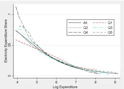
The essential difference between the AIDS and the QUAIDS model relates to the spec-ification of the relationship between expenditure on goods in the system and income, commonly represented as Engel curves. If households of different income levels react (via their expenditure on certain goods) differently to a change in their income, then the AIDS formulation will not capture these effects, but the QUAIDS model will. In our dataset, we can see from Figure 1 and 2 that both electricity and natural gas have Engel Curves which exhibit non–linearities even when the data are split out by income quintile; ex–ante motivating the selection of the QUAIDS model4_{. Ex-post consideration of the} model results will determine whether this is indeed appropriate.

[Figure 1 - 2 about here.]

4

(13)

In order to capture these non-linearities, Banks et al. (1997), extend Equation 3 to give: wi =αi+ n X j γijlnpj+βilog m a(p) + λi b(p) ln m a(p) 2 (5)

where a(p) = α0 +Pn_i₌₁αilnpi and b(p) = Qn_i₌₁pβii (the Cobb-Douglas price

aggre-gator). The first two terms are the same in Equations 3 and 5, the difference is the alteration of the specification of the impact of income on expenditure shares. In Equa-tion 3 expenditure is linear in income. In EquaEqua-tion 5 the linear term is still there, but there is an additional non-linear term _bλi₍_p₎

ln m a(p) 2

to capture non-linearities in the impact of income on expenditure shares. Note, importantly, that this non-linear term depends explicitly on prices. This means that the Engel curves for different goods can take different forms, better reflecting observed heterogeneity.

In order to capture differences between households which, for example, are based on demographic characteristics, requires expenditure shares which depend upon these characteristics. This has been outlined by Poi (2002). The essential modification adds into equation 5 a term to scale the expenditure function. This is best explained as follows. First we defineeR₍_p_,_u_{) as the household expenditure function and} _z_{as a vector}

of household characteristics. We then define a new function m0(p,z, u) = ¯m0(z) ×

φ(p,z, u). This can then be used to produce a new expenditure function e(p,z, u) =

m0(p,z, u) ×eR(p, u) which scales household expenditure according to some function of its characteristics z. Central to this scaling are the two terms ¯m0(z) and φ(p,z, u), which we now define. The first, ¯m0(z) = 1 +ρ′z depends on the vector of household characteristics and some estimated parameters, basically estimating the effect of these characteristics on household expenditure. The second, φ(p,z, u), captures changes in relative prices and differences in the composition of expenditure across different types of goods by households. In practice this is parametrised as:

(14)

lnφ(p,z, u) = Qk j=1p βj j ( Qk j=1p η′_jz j )−1 1 u − Pk j=1λjlnpj (6) This enables the introduction of this scaling by the demographic characteristics into the expenditure share equation (Equation 5 above) as follows:

wi =αi+ n X j γijlnpj+ (βi+η ′ iz) log m ¯ m0(z)a(p) + λi b(p)c(p,z) ln m ¯ m0(z)a(p) 2 (7) where c(p,z) = Qn j p η′_jz j .

Equation 7 makes clear how this scaling by household characteristics is implemented into the demand system affecting both the linear and quadratic expenditure terms. This provides us with a model which allows for differences in the shape of the Engel curves for different goods, and allows us to control for the characteristics of each household in estimating their responsiveness to changes in prices. This QUAIDS model is the model which we will implement later in this paper. Having outlined the AIDS and QUAIDS model, the final element to review is how one calculates the elasticities in such a model. The next section outlines the calculation of the compensated (Hicksian) and uncompensated (Marshallian) price elasticities of demand, and the income (expenditure) elasticity of demand.

3.3

Price elasticities

Having estimated this model the main task is to calculate price and income elasticities of demand. This section details how this is done for both the compensated and uncom-pensated elasticities of demand. Hicksian (comuncom-pensated) elasticities of demand differ from Marshallian (uncompensated) elasticities of demand in that the former keep the consumers’ utility constant while the latter keeps her income constant. The term com-pensated refers to the assumption that we make in the Hicksian case that the consumer

(15)

receives a compensation in their income in response to the price change to maintain the initial utility level. In practice what this means is that the compensated elasticity reflects only the substitution effect, unlike the uncompensated elasticity of demand which also includes an income effect.

The uncompensated price elasticity of demand for the QUAIDS model is:

ǫij =−δij + 1 wi γij − βi +η ′ iz+ 2λi b(p)c(p, z)ln m ¯ m0(z)a(p) x αj + X l γjllnpl − (βj +η ′ jz)λi b(p)c(p, z) ln m ¯ m0(z)a(p) 2 (8)

While the compensated price elasticities of demand are obtained through application of the Slutsky equation:

ǫCij =ǫij +µiwj (9)

The income (expenditure) elasticities of demand are calculated as:

µi = 1 + 1 wi βi+η ′ iz+ 2λi b(p)c(p, z)ln m ¯ m0(z)a(p) (10) Having outlined the demand system, and the calculation of each of the key elasticities, the next section describes the data used in this empirical exercise.

4

Data and estimation

The data used in this paper come primarily from the Living Cost and Food Survey (previously known as Expenditure and Food Survey) produced annually by the UK Office of National Statistics. The questions in the survey cover a range of topics related to the household. These include: household income, expenditure by the household on different goods and services, and housing details. In this study we use data from this survey for

(16)

the period covering 2007-2014. We extract from the survey data information related to the energy consumption of households, household demographic characteristics, housing characteristics (including ownership of domestic appliances), and household income. A summary of the variables extracted from the survey is contained in Table 1.

[ Table 1 about here ]

In selecting household characteristics to include in the QUAIDS model our starting point was the factors controlled for in Baker et al. (1989). While a quarter of a century have passed since its publication, Baker et al. (1989) provides an useful starting point in the exploration of these same issues in this present study. In updating these control variables, we added household ownership of televisions, dishwashers and internet connec-tion. Figure 3 demonstrates the change, and in some cases lack of change, in appliance ownership by UK Households over the 5 decades to 2014. We can see the emergence of washing machines as a household staple, the ever presence of televisions in households, and the more recent developments in tumble dryer, DVD player, dish-washer, microwave and computer ownership.

[ Tables 2 - 3 about here ]

In addition to those data taken from the Living Cost and Food Survey, this paper utilised information on the average temperature in each region of the UK in each of the quarters during which measurements of income and expenditure were taken. These data came from the UK Meteorological Office or ‘Met Office’, and enabled us to match each quarter-region data entry with the appropriate average outside air temperature. Data on gas prices, electricity prices, and the general price level were taken from the UK Department of Energy & Climate Change. Descriptive statistics for each of the variables, by year, are contained in Table 2.

(17)

These models have traditionally been estimated by maximum likelihood, for example using commands written by Poi (2002). More recently there has been a move to use nonlinear seemingly unrelated regression to estimate these demand systems for largely computational reasons (e.g. Poi (2008, 2012))5_{. This is the approach used in this paper} where we estimate the quadratic version of the AIDS model developed by Banks et al. (1997), outlined earlier. Finally, given the inclusion of a regional level covariates in these estimation (the temperature variable), cluster robust standard errors are used in all estimations. The next section presents our estimation results.

5

Results

This section is structured into two parts. First, we review the results for the whole of Great Britain, varying the price vector that is used for electricity and gas. Second, we present our estimates of the elasticity of demand for each of five income quintiles. We focus on the elasticity estimates derived from these results using the formula outlined earlier rather than discussing individual model parameter estimates, although these are available on request and were sent to the referees. The only element which we will comment directly on here is that the coefficients (λ) on the non–linear income term for all three goods (electricity, gas and non-energy) are all highly significant for all our models, justifying the selection of the QUAIDS and not the AIDS model in our analysis.

5.1

Price elasticities of demand using different price lags

We outlined earlier that it has typically been assumed in the literature that the rele-vant reference price when estimating elasticities of demand for electricity and gas is the contemporaneous electricity and gas price. The sensitivity of empirical results to this assumption, to our knowledge, has never been tested. There are a number of reasons to question this assumption. The first, and most obvious, is that with the exception

5

It is perhaps worth noting that, as Poi (2012) points out, this approach is: “equivalent to the multivariate normal maximum-likelihood estimator for this class of problems”.

(18)

of customers on pre-payment meters (15% of UK electricity consumers6_{) and those just} getting access to smart meters (just over 3% of UK electricity and gas consumers by the end of 20147_{), consumers do not observe electricity prices contemporaneously. The} second, is that consumers on direct debit and credit meters typically receive bills with a lag, thus the ‘signal’ that they receive about the cost of their electricity and/or gas use is received with some delay after the quarter in which they consume that electricity and/or gas. Finally, even if one believed that consumers track the wholesale price of electricity contemporaneously, they are not billed on the basis of these prices.

For these reasons, we begin our analysis of how households respond to changing elec-tricity and gas prices by considering the elasticity of household elecelec-tricity and gas demand with respect to different reference prices, namely: contemporaneous prices, with a one quarter lag, with a two quarter lag, with a three quarter lag, and with a four quarter lag. Table 4 presents the results from our model of the price elasticity of demand for electricity and gas using these different reference prices.

[ Tables 4 & 5 about here ]

Results are presented for the compensated and uncompensated elasticities of demand for completeness, but they are broadly similar and we focus in this section on the com-pensated elasticity of demand results. We can see that for Gas, the contemporaneous price elasticity of demand for GB households is -0.655, suggesting that a 1% increase in gas prices reduces gas consumption, on average in GB, by 0.655%. This estimate is statistically significantly different from zero with a t-statistic in excess of 9.6. If instead of using the contemporaneous price we instead look at the price lagged by one quarter, we can see that the elasticity estimate drops to 0.546, with a two quarter lag in the price we can see that the elasticity falls slightly again to -0.514, thereafter (with a three and four quarter lag) the elasticity increases with it’s highest value with respect to gas prices four quarters before.

6

https://www.gov.uk/government/statistical-data-sets/quarterly-domestic-energy-price-stastics\#history

7

(19)

For electricity, a similar pattern is observed with the contemporaneous elasticity of demand estimate (-0.357) higher than the elasticity with respect to prices in the quar-ter before (-0.350) and two quarquar-ters before (-0.251, albeit only statistically significantly different from zero at the 10% level) before increasing again with respect to prices three (-0.493) and four quarters before (-0.876). In terms of the cross price elasticity of demand between electricity and gas, we can see that the cross price elasticity estimates, unlike Baker et al. (1989), have a consistent sign and indicate that these goods are comple-ments. However, only with respect to prices lagged by two quarters are these estimates statistically significantly different from zero, and then only at the 10% level.

These results show two things. Firstly, they provide useful information on how GB households’ electricity and gas demands respond to electricity and gas prices. Secondly, these results suggest that the common use of contemporaneous prices in the estimation of household elasticities for electricity and gas may be over-estimating the size of the response of demand to changes in prices if the prices that consumers actually observe and respond to are the prices in the quarter or two quarters before (and underestimating the magnitude of the response if the relevant price signal is three or four quarters before). There are good reasons, outlined earlier, to believe that in the UK the relevant price signal for households is not contemporaneous. Which alternative one should use, absent a more formal test, is something that each analyst should decide upon, although we do not think it likely that households take a full year to recognise electricity/gas prices changing, and with billing typically lagged by a quarter, we would tend to use the estimates lagged by at least a quarter and more likely two quarters. In the next set of results we focus on the results from our model with the best log-likelihood which is the results using price data lagged by two quarters.

5.2

Price elasticities of demand across the income distribution

Key to understanding the distributional impacts of a range of energy policies which affect the price that consumers pay for electricity and gas is understanding how the value of

(20)

the price elasticity of demand changes across the income distribution. These results are presented in Tables 6 & 7.

[ Tables 6 & 7 about here ]

For natural gas, as we move from the lowest income quintile group to the highest income quintile group the elasticity of demand with respect to the price, while inelastic in all cases, becomes less so. Given that gas is used by households primarily for heating and cooking, it makes sense that the poorest households have the most inelastic demand for gas; with a 1% increase in gas price reducing gas consumption on average among this group by 0.394%. This estimate is barely insignificant at the 10% level, this means that for the poorest households we cannot conclude that their elasticity of demand for gas is anything other than perfectly inelastic (elasticity estimate of zero) based on these results. For all other income groups, gas consumption appears to respond inelastically to changes in gas prices, with households in the second income quintile on average reducing consumption of gas by 0.432% in response to a 1% increase in gas prices. This compares to the highest income households who, on average, would reduce their gas consumption by 0.698% in response to the same change in gas prices.

For electricity a similar pattern emerges of lower income households having less elastic demand than higher income households. Here we find that electricity demand for the three lowest income quintiles in GB is inelastic with respect to changes in electricity prices, and with low t-statistic scores we must accept the null hypothesis that these elasticities are not statistically significantly different from zero and thus demand is perfectly inelastic. For higher income households demand is similarly inelastic, although less so for the highest income group (-0.705) relative to the second highest income quintile (-0.450).

These results suggest that changes in energy policy which have the effect of raising electricity and gas prices will raise revenue, given that demand is inelastic, and may be attractive to government for that reason. However, what these results also demonstrate is that it will do so in a way which impacts most acutely on the poorest income households.

(21)

Given the important role of electricity and gas in everyday life, in providing heating, cooking and use of basic household appliances, it isn’t a surprise that the poorest house-holds are less able to change their demand for energy in response to changing electricity and gas prices. It therefore remains a puzzle why much of energy policy in the U.K. focuses on measures which will increase energy prices, or will have the effect of doing so, without an associated focus on helping the poorest households who are disproportionately affected by these measures as these results illustrate.

6

Conclusions

This article has produced up-to-date estimates of household elasticity of demand for elec-tricity and gas using microdata for Great Britain as a whole under different reference prices and across the income distribution; updating and extending Baker et al. (1989). In doing so, we have established that using contemporaneous electricity and gas prices produces higher estimates of the household price elasticity of demand than those pro-duced using lagged prices from the quarter or two quarters before (and conversely lower estimates than those produced using prices from three or four quarters before). It is not clear, ex-ante, which of these alternative price signals is the relevant one for households in making decisions about energy consumption, however we have argued that since house-holds generally do not observe prices contemporaneously then analysts seeking short term elasticity estimates should not use estimates produced on this basis.

Given the importance of price -directly and indirectly- in delivering UK energy policy objectives, we also explored whether there are differences in the how households respond to changes in electricity and gas prices over the income distribution. We found that for the lowest income households their gas demand responded less to changes in gas prices than higher income households, while for households in the lowest income quintile their demand for gas appears to be perfectly inelastic. For electricity, we found that for the bottom three income quintiles their elasticity of demand was statistically insignificantly different

(22)

from zero (i.e. perfectly inelastic). With the lowest income households having short-run elasticities of demand which are not statistically significantly different from zero, it is clear that increases in energy prices will disproportionately affect the households budgets of the poorest households. The results of this analysis demonstrate that the use of price as an instrument -directly and indirectly- of energy policy something which will have profound distributional impacts.

(23)

Figure 1: Engel Curve for Electricity

(24)

a

Figure 3: UK Appliance Ownership by households, 1973-2014

a_{Source: Department of Energy & Climate Change: ‘Energy Consumption in the UK Domestic data}

(25)

V ar iab le n am e D efi n it ion Y ear S ou rc e G E XP S H G as ex p en d it u re /t ot al ex p en d it u re 2007-2014 C al cu lat ed b y au th or fr om Li v in g C os ts an d F o o d S u rv ey d at a E LE XP S H E le ct ri ci ty ex p en d it u re /t ot al ex p en d it u re 2007-2014 C al cu lat ed b y au th or fr om Li v in g C os ts an d F o o d S u rv ey d at a NE NE R Non -e n er gy ex p en d it u re /t ot al ex p en d it u re 2007-2014 C al cu lat ed b y au th or fr om Li v in g C os ts an d F o o d S u rv ey d at a E P IXY E le ct ri ci ty p ri ce 2007-2014 O ffi ce for Nat ion al S tat is ti cs C P IH In d ex 04. 5. 1: E le ct ri ci ty G P IXY G as p ri ce 2007-2014 O ffi ce for Nat ion al S tat is ti cs C P IH In d ex 04. 5. 2: G as F P IXP P ri ce of n on -e n er gy go o d s 2007-2014 O ffi ce for Nat ion al S tat is ti cs C P IH In d ex : E x cl u d in g en er gy P 600 T ot al HH ex p en d it u re 2007-2014 Li v in g C os ts an d F o o d S u rv ey log INC O M E log of n or m al w ee k ly d is p os ab le h ou se h ol d in com e 2007-2014 Li v in g C os ts an d F o o d S u rv ey logHS IZ E log of n u m b er of p eop le in th e h ou se h ol d 2007-2014 Li v in g C os ts an d F o o d S u rv ey K ID S D = 1 if th er e ar e ch il d re n u n d er 5 y ear s ol d in HH 2007-2014 Li v in g C os ts an d F o o d S u rv ey HAD UL T = 1 if an y ad u lt in HH is ou t of lab ou r for ce 2007-2014 Li v in g C os ts an d F o o d S u rv ey A G E 40 = 1 if HH h ead is age d > 40 2007-2014 Li v in g C os ts an d F o o d S u rv ey A G E 65 = 1 if HH h ead is age d > 65 2007-2014 Li v in g C os ts an d F o o d S u rv ey logR O O M S log of n u m b er of ro om s in th e ac com m o d at ion 2007-2014 Li v in g C os ts an d F o o d S u rv ey E LE C T O NL Y E le ct ri ci ty on ly in th e HH 2007-2014 Li v in g C os ts an d F o o d S u rv ey G C H G as ce n tr al h eat in g in HH 2007-2014 Li v in g C os ts an d F o o d S u rv ey E C H E le ct ri c ce n tr al h eat in g in HH 2007-2014 Li v in g C os ts an d F o o d S u rv ey O C H O il ce n tr al h eat in g in HH 2007-2014 Li v in g C os ts an d F o o d S u rv ey T E M P Av er age ou ts id e te m p er at u re in th e re gi on an d q u ar te r of ex p en d it u re 2007-2014 http://www.metoffice.gov.uk/climate/uk/summaries/datasets W AS H = 1 if th er e is a w as h in g m ac h in e in th e ac com m o d at ion 2007-2014 Li v in g C os ts an d F o o d S u rv ey F R ID G E = 1 if th er e is a fr id ge in th e ac com m o d at ion 2007-2014 Li v in g C os ts an d F o o d S u rv ey T E LE = 1 if th er e is a te le v is ion in th e ac com m o d at ion 2007-2014 Li v in g C os ts an d F o o d S u rv ey D IS H = 1 if th er e is a d is h w as h er in th e ac com m o d at ion 2007-2014 Li v in g C os ts an d F o o d S u rv ey W W W = 1 if th er e is in te rn et ac ce ss in th e ac com m o d at ion 2007-2014 L iv in g C os ts an d F o o d S u rv ey C O UNC IL = 1 if ac com m o d at ion is re n te d fr om lo cal au th or it y 2007-2014 Li v in g C os ts an d F o o d S u rv ey R E NT = 1 if ac com m o d at ion is p ri vat el y re n te d 2007-2014 Li v in g C os ts an d F o o d S u rv ey R E NT F R E E = 1 if ac com m o d at ion is li v ed in re n t fr ee 2007-2014 Li v in g C os ts an d F o o d S u rv ey O W NC O M P = 1 if ac com m o d at ion is ow n ed ou tr igh t 2007-2014 Li v in g C os ts an d F o o d S u rv ey S P R A UT = 1 if ex p en d it u re in Ap ri l-J u n e or O ct ob er -D ec em b er 2007-2014 Li v in g C os ts an d F o o d S u rv ey S UM M E R = 1 if ex p en d it u re in J u ly -S ep te m b er 2007-2014 Li v in g C os ts an d F o o d S u rv ey R E G IO N2-R E G IO N 11 R egi on al F ix ed E ff ec ts 2007-2014 Li v in g C os ts an d F o o d S u rv ey T ab le 1: V ar ia b le d et ai ls

(26)

W h o le S a mp le Q u in ti le 1 Q u in ti le 2 V a ri a b le O b s M e a n S td . D e v . M in M a x O b s M e a n S td . D e v . M in M a x O b s M e a n S td . D e v . M in M a x G a s E x p S h a re 4 1 ,4 2 9 0 .0 3 1 0 .0 3 4 0 .0 0 0 0 .2 5 0 7 ,8 7 1 0 .0 4 2 0 .0 4 9 0 .0 0 0 0 .2 5 0 8 ,6 5 5 0 .0 3 6 0 .0 3 7 0 .0 0 0 0 .2 5 0 E le c E x p S h a re 4 1 ,4 2 9 0 .0 3 1 0 .0 2 9 0 .0 0 0 0 .2 4 9 7 ,8 7 1 0 .0 4 3 0 .0 4 2 0 .0 0 0 0 .2 4 9 8 ,6 5 5 0 .0 3 6 0 .0 3 2 0 .0 0 0 0 .2 4 9 N o n -E n e rg y E x p S h a re 4 1 ,4 2 9 0 .9 3 7 0 .0 5 4 0 .5 0 4 1 .0 0 0 7 ,8 7 1 0 .9 1 5 0 .0 7 7 0 .5 0 4 1 .0 0 0 8 ,6 5 5 0 .9 2 8 0 .0 5 8 0 .5 2 4 1 .0 0 0 G a s P ri c e 4 1 ,4 2 9 0 .7 6 8 0 .1 4 1 0 .5 3 4 1 .0 0 6 7 ,8 7 1 0 .7 6 7 0 .1 4 0 0 .5 3 4 1 .0 0 6 8 ,6 5 5 0 .7 6 8 0 .1 4 1 0 .5 3 4 1 .0 0 6 E le c P ri c e 4 1 ,4 2 9 0 .8 1 0 0 .1 0 4 0 .6 3 3 1 .0 0 7 7 ,8 7 1 0 .8 0 9 0 .1 0 4 0 .6 3 3 1 .0 0 7 8 ,6 5 5 0 .8 1 0 0 .1 0 4 0 .6 3 3 1 .0 0 7 N o n -E n e rg y P ri c e 4 1 ,4 2 9 0 .9 1 4 0 .0 5 1 0 .8 3 4 1 .0 0 0 7 ,8 7 1 0 .9 1 4 0 .0 5 1 0 .8 3 4 1 .0 0 0 8 ,6 5 5 0 .9 1 5 0 .0 5 2 0 .8 3 4 1 .0 0 0 T o ta l E x p e n d it u re 4 1 ,4 2 9 4 1 2 .1 4 5 3 2 5 .3 7 5 5 0 .0 3 5 9 3 9 4 .7 2 0 7 ,8 7 1 1 8 9 .2 0 0 1 4 9 .0 5 6 5 0 .0 3 5 3 1 0 4 .5 2 5 8 ,6 5 5 2 7 9 .8 2 7 1 7 3 .2 2 1 5 0 .2 9 5 3 3 6 5 .9 5 5 lo g (I n c o me ) 4 1 ,4 2 9 6 .0 9 8 0 .7 2 8 -3 .2 1 9 7 .3 9 7 7 ,8 7 1 5 .0 1 1 0 .5 3 3 -3 .2 1 9 5 .6 2 4 8 ,6 5 5 5 .7 4 2 0 .1 5 8 5 .3 9 3 6 .1 0 0 lo g (# p e o p le in H H ) 4 1 ,4 2 9 0 .7 2 3 0 .5 2 5 0 .0 0 0 2 .1 9 7 7 ,8 7 1 0 .2 7 9 0 .4 3 2 0 .0 0 0 2 .1 9 7 8 ,6 5 5 0 .5 6 6 0 .4 9 2 0 .0 0 0 2 .1 9 7 C h il d < 5 in H H 4 1 ,4 2 9 0 .1 2 3 0 .3 2 8 0 .0 0 0 1 .0 0 0 7 ,8 7 1 0 .0 7 7 0 .2 6 7 0 .0 0 0 1 .0 0 0 8 ,6 5 5 0 .0 9 6 0 .2 9 5 0 .0 0 0 1 .0 0 0 H A D U L T 4 1 ,4 2 9 0 .0 6 5 0 .2 4 7 0 .0 0 0 1 .0 0 0 7 ,8 7 1 0 .1 1 4 0 .3 1 8 0 .0 0 0 1 .0 0 0 8 ,6 5 5 0 .0 6 6 0 .2 4 8 0 .0 0 0 1 .0 0 0 A G E 4 0 4 1 ,4 2 9 0 .7 5 7 0 .4 2 9 0 .0 0 0 1 .0 0 0 7 ,8 7 1 0 .8 1 7 0 .3 8 7 0 .0 0 0 1 .0 0 0 8 ,6 5 5 0 .7 9 4 0 .4 0 4 0 .0 0 0 1 .0 0 0 A G E 6 5 4 1 ,4 2 9 0 .2 7 8 0 .4 4 8 0 .0 0 0 1 .0 0 0 7 ,8 7 1 0 .4 4 1 0 .4 9 7 0 .0 0 0 1 .0 0 0 8 ,6 5 5 0 .4 2 8 0 .4 9 5 0 .0 0 0 1 .0 0 0 lo g (# ro o ms in H H ) 4 1 ,4 2 9 1 .6 1 4 0 .2 3 3 0 .0 0 0 1 .7 9 2 7 ,8 7 1 1 .4 7 5 0 .2 8 2 0 .0 0 0 1 .7 9 2 8 ,6 5 5 1 .5 7 0 0 .2 4 3 0 .0 0 0 1 .7 9 2 O n ly E le c in H H 4 1 ,4 2 9 0 .1 4 4 0 .3 5 1 0 .0 0 0 1 .0 0 0 7 ,8 7 1 0 .1 8 2 0 .3 8 6 0 .0 0 0 1 .0 0 0 8 ,6 5 5 0 .1 6 0 0 .3 6 6 0 .0 0 0 1 .0 0 0 G a s C e n tr a l H e a ti n g 4 1 ,4 2 9 0 .8 2 1 0 .3 8 4 0 .0 0 0 1 .0 0 0 7 ,8 7 1 0 .7 6 8 0 .4 2 2 0 .0 0 0 1 .0 0 0 8 ,6 5 5 0 .7 9 8 0 .4 0 1 0 .0 0 0 1 .0 0 0 E le c C e n tr a l H e a ti n g 4 1 ,4 2 9 0 .0 6 9 0 .2 5 3 0 .0 0 0 1 .0 0 0 7 ,8 7 1 0 .1 1 9 0 .3 2 4 0 .0 0 0 1 .0 0 0 8 ,6 5 5 0 .0 9 1 0 .2 8 8 0 .0 0 0 1 .0 0 0 O il C e n tr a l H e a ti n g 4 1 ,4 2 9 0 .0 6 9 0 .2 5 3 0 .0 0 0 1 .0 0 0 7 ,8 7 1 0 .0 4 9 0 .2 1 6 0 .0 0 0 1 .0 0 0 8 ,6 5 5 0 .0 5 9 0 .2 3 6 0 .0 0 0 1 .0 0 0 R e g io n a l T e mp e ra tu re 4 1 ,4 2 9 9 .7 1 2 4 .0 8 8 1 .5 0 0 1 6 .9 0 0 7 ,8 7 1 9 .6 3 6 4 .0 9 9 1 .5 0 0 1 6 .9 0 0 8 ,6 5 5 9 .6 4 1 4 .0 4 6 1 .5 0 0 1 6 .9 0 0 W a sh in g M a c h in e in H H 4 1 ,4 2 9 0 .9 7 0 0 .1 7 2 0 .0 0 0 1 .0 0 0 7 ,8 7 1 0 .9 0 5 0 .2 9 3 0 .0 0 0 1 .0 0 0 8 ,6 5 5 0 .9 6 4 0 .1 8 6 0 .0 0 0 1 .0 0 0 F ri d g e in H H 4 1 ,4 2 9 0 .9 7 6 0 .1 5 2 0 .0 0 0 1 .0 0 0 7 ,8 7 1 0 .9 4 7 0 .2 2 4 0 .0 0 0 1 .0 0 0 8 ,6 5 5 0 .9 7 3 0 .1 6 1 0 .0 0 0 1 .0 0 0 T e le v is io n in H H 4 1 ,4 2 9 0 .9 8 5 0 .1 2 1 0 .0 0 0 1 .0 0 0 7 ,8 7 1 0 .9 7 4 0 .1 5 8 0 .0 0 0 1 .0 0 0 8 ,6 5 5 0 .9 8 5 0 .1 2 0 0 .0 0 0 1 .0 0 0 D is h w a sh e r in H H 4 1 ,4 2 9 0 .4 1 8 0 .4 9 3 0 .0 0 0 1 .0 0 0 7 ,8 7 1 0 .1 5 8 0 .3 6 5 0 .0 0 0 1 .0 0 0 8 ,6 5 5 0 .2 6 9 0 .4 4 3 0 .0 0 0 1 .0 0 0 In te rn e t in H H 4 1 ,4 2 9 0 .7 5 5 0 .4 3 0 0 .0 0 0 1 .0 0 0 7 ,8 7 1 0 .4 3 0 0 .4 9 5 0 .0 0 0 1 .0 0 0 8 ,6 5 5 0 .6 2 8 0 .4 8 3 0 .0 0 0 1 .0 0 0 P ro p e rt y re n te d fr o m C o u n c il 4 1 ,4 2 9 0 .1 6 6 0 .3 7 2 0 .0 0 0 1 .0 0 0 7 ,8 7 1 0 .3 9 6 0 .4 8 9 0 .0 0 0 1 .0 0 0 8 ,6 5 5 0 .2 3 4 0 .4 2 4 0 .0 0 0 1 .0 0 0 P ro p e rt y R e n te d P ri v a te ly 4 1 ,4 2 9 0 .1 2 7 0 .3 3 3 0 .0 0 0 1 .0 0 0 7 ,8 7 1 0 .1 5 9 0 .3 6 5 0 .0 0 0 1 .0 0 0 8 ,6 5 5 0 .1 4 3 0 .3 5 0 0 .0 0 0 1 .0 0 0 H H L iv e s R e n t F re e 4 1 ,4 2 9 0 .0 1 1 0 .1 0 6 0 .0 0 0 1 .0 0 0 7 ,8 7 1 0 .0 1 8 0 .1 3 2 0 .0 0 0 1 .0 0 0 8 ,6 5 5 0 .0 1 4 0 .1 1 9 0 .0 0 0 1 .0 0 0 P ro p e rt y O w n e d O u tr ig h t 4 1 ,4 2 9 0 .3 4 2 0 .4 7 4 0 .0 0 0 1 .0 0 0 7 ,8 7 1 0 .3 4 8 0 .4 7 6 0 .0 0 0 1 .0 0 0 8 ,6 5 5 0 .4 2 7 0 .4 9 5 0 .0 0 0 1 .0 0 0 S p ri n g / A u tu mn 4 1 ,4 2 9 0 .5 0 0 0 .5 0 0 0 .0 0 0 1 .0 0 0 7 ,8 7 1 0 .4 9 4 0 .5 0 0 0 .0 0 0 1 .0 0 0 8 ,6 5 5 0 .5 0 4 0 .5 0 0 0 .0 0 0 1 .0 0 0 S u mme r 4 1 ,4 2 9 0 .2 5 4 0 .4 3 5 0 .0 0 0 1 .0 0 0 7 ,8 7 1 0 .2 5 6 0 .4 3 7 0 .0 0 0 1 .0 0 0 8 ,6 5 5 0 .2 4 7 0 .4 3 2 0 .0 0 0 1 .0 0 0 T ab le 2: D es cr ip ti ve S ta ti st ic s 1

(27)

Q u in ti le 3 Q u in ti le 4 Q u in ti le 5 V a ri a b le O b s M e a n S td . D e v . M in M a x O b s M e a n S td . D e v . M in M a x O b s M e a n S td . D e v . M in M a x G a s E x p S h a re 8 ,5 5 6 0 .0 3 0 0 .0 2 8 0 .0 0 0 0 .2 4 9 8 ,2 5 8 0 .0 2 6 0 .0 2 4 0 .0 0 0 0 .2 4 8 8 ,0 8 9 0 .0 2 2 0 .0 2 0 0 .0 0 0 0 .2 2 9 E le c E x p S h a re 8 ,5 5 6 0 .0 3 0 0 .0 2 5 0 .0 0 0 0 .2 3 6 8 ,2 5 8 0 .0 2 6 0 .0 2 0 0 .0 0 0 0 .2 4 7 8 ,0 8 9 0 .0 2 2 0 .0 1 7 0 .0 0 0 0 .2 1 3 N o n -E n e rg y E x p S h a re 8 ,5 5 6 0 .9 4 0 0 .0 4 4 0 .5 4 6 1 .0 0 0 8 ,2 5 8 0 .9 4 8 0 .0 3 7 0 .5 6 7 1 .0 0 0 8 ,0 8 9 0 .9 5 6 0 .0 3 0 0 .6 4 8 1 .0 0 0 G a s P ri c e 8 ,5 5 6 0 .7 6 9 0 .1 4 1 0 .5 3 4 1 .0 0 6 8 ,2 5 8 0 .7 6 7 0 .1 4 1 0 .5 3 4 1 .0 0 6 8 ,0 8 9 0 .7 6 9 0 .1 4 1 0 .5 3 4 1 .0 0 6 E le c P ri c e 8 ,5 5 6 0 .8 1 1 0 .1 0 4 0 .6 3 3 1 .0 0 7 8 ,2 5 8 0 .8 0 9 0 .1 0 4 0 .6 3 3 1 .0 0 7 8 ,0 8 9 0 .8 1 0 0 .1 0 4 0 .6 3 3 1 .0 0 7 N o n -E n e rg y P ri c e 8 ,5 5 6 0 .9 1 5 0 .0 5 2 0 .8 3 4 1 .0 0 0 8 ,2 5 8 0 .9 1 4 0 .0 5 1 0 .8 3 4 1 .0 0 0 8 ,0 8 9 0 .9 1 5 0 .0 5 1 0 .8 3 4 1 .0 0 0 T o ta l E x p e n d it u re 8 ,5 5 6 3 7 9 .0 8 1 2 2 2 .2 7 8 5 6 .2 1 5 8 7 8 8 .7 5 0 8 ,2 5 8 4 8 8 .7 9 5 2 4 7 .3 2 5 5 0 .5 9 5 3 6 8 1 .9 6 0 8 ,0 8 9 7 2 7 .3 8 1 4 4 7 .4 3 3 6 0 .1 3 0 9 3 9 4 .7 2 0 lo g (I n c o me ) 8 ,5 5 6 6 .1 6 3 0 .1 2 5 5 .8 9 6 6 .4 5 8 8 ,2 5 8 6 .5 3 4 0 .1 2 2 6 .2 7 9 6 .8 3 8 8 ,0 8 9 7 .0 2 4 0 .1 9 9 6 .6 6 6 7 .3 9 7 lo g (# p e o p le in H H ) 8 ,5 5 6 0 .7 8 0 0 .4 7 3 0 .0 0 0 2 .1 9 7 8 ,2 5 8 0 .9 3 3 0 .4 3 9 0 .0 0 0 2 .1 9 7 8 ,0 8 9 1 .0 4 8 0 .4 0 5 0 .0 0 0 2 .1 9 7 C h il d < 5 in H H 8 ,5 5 6 0 .1 3 5 0 .3 4 1 0 .0 0 0 1 .0 0 0 8 ,2 5 8 0 .1 5 4 0 .3 6 1 0 .0 0 0 1 .0 0 0 8 ,0 8 9 0 .1 5 0 0 .3 5 7 0 .0 0 0 1 .0 0 0 H A D U L T 8 ,5 5 6 0 .0 5 6 0 .2 3 0 0 .0 0 0 1 .0 0 0 8 ,2 5 8 0 .0 5 1 0 .2 2 1 0 .0 0 0 1 .0 0 0 8 ,0 8 9 0 .0 4 0 0 .1 9 7 0 .0 0 0 1 .0 0 0 A G E 4 0 8 ,5 5 6 0 .7 3 3 0 .4 4 3 0 .0 0 0 1 .0 0 0 8 ,2 5 8 0 .6 9 7 0 .4 5 9 0 .0 0 0 1 .0 0 0 8 ,0 8 9 0 .7 4 4 0 .4 3 6 0 .0 0 0 1 .0 0 0 A G E 6 5 8 ,5 5 6 0 .2 7 6 0 .4 4 7 0 .0 0 0 1 .0 0 0 8 ,2 5 8 0 .1 5 4 0 .3 6 1 0 .0 0 0 1 .0 0 0 8 ,0 8 9 0 .0 9 0 0 .2 8 6 0 .0 0 0 1 .0 0 0 lo g (# ro o ms in H H ) 8 ,5 5 6 1 .6 2 8 0 .2 1 0 0 .0 0 0 1 .7 9 2 8 ,2 5 8 1 .6 7 1 0 .1 8 0 0 .6 9 3 1 .7 9 2 8 ,0 8 9 1 .7 2 5 0 .1 4 7 0 .0 0 0 1 .7 9 2 O n ly E le c in H H 8 ,5 5 6 0 .1 3 3 0 .3 4 0 0 .0 0 0 1 .0 0 0 8 ,2 5 8 0 .1 2 2 0 .3 2 7 0 .0 0 0 1 .0 0 0 8 ,0 8 9 0 .1 2 4 0 .3 3 0 0 .0 0 0 1 .0 0 0 G a s C e n tr a l H e a ti n g 8 ,5 5 6 0 .8 3 2 0 .3 7 4 0 .0 0 0 1 .0 0 0 8 ,2 5 8 0 .8 4 9 0 .3 5 8 0 .0 0 0 1 .0 0 0 8 ,0 8 9 0 .8 5 4 0 .3 5 3 0 .0 0 0 1 .0 0 0 E le c C e n tr a l H e a ti n g 8 ,5 5 6 0 .0 6 0 0 .2 3 8 0 .0 0 0 1 .0 0 0 8 ,2 5 8 0 .0 4 5 0 .2 0 7 0 .0 0 0 1 .0 0 0 8 ,0 8 9 0 .0 3 1 0 .1 7 2 0 .0 0 0 1 .0 0 0 O il C e n tr a l H e a ti n g 8 ,5 5 6 0 .0 6 8 0 .2 5 1 0 .0 0 0 1 .0 0 0 8 ,2 5 8 0 .0 7 3 0 .2 6 0 0 .0 0 0 1 .0 0 0 8 ,0 8 9 0 .0 9 4 0 .2 9 2 0 .0 0 0 1 .0 0 0 R e g io n a l T e mp e ra tu re 8 ,5 5 6 9 .6 6 2 4 .1 0 0 1 .5 0 0 1 6 .9 0 0 8 ,2 5 8 9 .7 1 2 4 .0 9 5 1 .5 0 0 1 6 .9 0 0 8 ,0 8 9 9 .9 1 7 4 .0 9 7 1 .5 0 0 1 6 .9 0 0 W a sh in g M a c h in e in H H 8 ,5 5 6 0 .9 8 6 0 .1 1 8 0 .0 0 0 1 .0 0 0 8 ,2 5 8 0 .9 9 3 0 .0 8 1 0 .0 0 0 1 .0 0 0 8 ,0 8 9 0 .9 9 7 0 .0 5 3 0 .0 0 0 1 .0 0 0 F ri d g e in H H 8 ,5 5 6 0 .9 8 4 0 .1 2 7 0 .0 0 0 1 .0 0 0 8 ,2 5 8 0 .9 8 6 0 .1 1 7 0 .0 0 0 1 .0 0 0 8 ,0 8 9 0 .9 9 0 0 .1 0 1 0 .0 0 0 1 .0 0 0 T e le v is io n in H H 8 ,5 5 6 0 .9 8 6 0 .1 1 8 0 .0 0 0 1 .0 0 0 8 ,2 5 8 0 .9 8 9 0 .1 0 6 0 .0 0 0 1 .0 0 0 8 ,0 8 9 0 .9 9 1 0 .0 9 5 0 .0 0 0 1 .0 0 0 D is h w a sh e r in H H 8 ,5 5 6 0 .3 9 3 0 .4 8 8 0 .0 0 0 1 .0 0 0 8 ,2 5 8 0 .5 2 8 0 .4 9 9 0 .0 0 0 1 .0 0 0 8 ,0 8 9 0 .7 4 6 0 .4 3 5 0 .0 0 0 1 .0 0 0 In te rn e t in H H 8 ,5 5 6 0 .8 1 7 0 .3 8 7 0 .0 0 0 1 .0 0 0 8 ,2 5 8 0 .9 2 1 0 .2 7 0 0 .0 0 0 1 .0 0 0 8 ,0 8 9 0 .9 7 0 0 .1 7 0 0 .0 0 0 1 .0 0 0 P ro p e rt y re n te d fr o m C o u n c il 8 ,5 5 6 0 .1 2 7 0 .3 3 3 0 .0 0 0 1 .0 0 0 8 ,2 5 8 0 .0 6 4 0 .2 4 5 0 .0 0 0 1 .0 0 0 8 ,0 8 9 0 .0 1 7 0 .1 2 8 0 .0 0 0 1 .0 0 0 P ro p e rt y R e n te d P ri v a te ly 8 ,5 5 6 0 .1 3 8 0 .3 4 5 0 .0 0 0 1 .0 0 0 8 ,2 5 8 0 .1 1 5 0 .3 1 9 0 .0 0 0 1 .0 0 0 8 ,0 8 9 0 .0 8 1 0 .2 7 3 0 .0 0 0 1 .0 0 0 H H L iv e s R e n t F re e 8 ,5 5 6 0 .0 0 9 0 .0 9 5 0 .0 0 0 1 .0 0 0 8 ,2 5 8 0 .0 0 9 0 .0 9 5 0 .0 0 0 1 .0 0 0 8 ,0 8 9 0 .0 0 7 0 .0 8 1 0 .0 0 0 1 .0 0 0 P ro p e rt y O w n e d O u tr ig h t 8 ,5 5 6 0 .3 8 6 0 .4 8 7 0 .0 0 0 1 .0 0 0 8 ,2 5 8 0 .2 8 7 0 .4 5 2 0 .0 0 0 1 .0 0 0 8 ,0 8 9 0 .2 5 7 0 .4 3 7 0 .0 0 0 1 .0 0 0 S p ri n g / A u tu mn 8 ,5 5 6 0 .4 9 7 0 .5 0 0 0 .0 0 0 1 .0 0 0 8 ,2 5 8 0 .4 9 5 0 .5 0 0 0 .0 0 0 1 .0 0 0 8 ,0 8 9 0 .5 0 7 0 .5 0 0 0 .0 0 0 1 .0 0 0 S u mme r 8 ,5 5 6 0 .2 5 5 0 .4 3 6 0 .0 0 0 1 .0 0 0 8 ,2 5 8 0 .2 5 5 0 .4 3 6 0 .0 0 0 1 .0 0 0 8 ,0 8 9 0 .2 5 8 0 .4 3 7 0 .0 0 0 1 .0 0 0 T ab le 3: D es cr ip ti ve S ta ti st ic s 2

(28)

a G a s P ri ce E le ct ri ci ty P ri ce C o n te m p . 1 Q la g 2 Q la g 3 Q la g 4 Q la g C o n te m p . 1 Q la g 2 Q la g 3 Q la g 4 Q la g Co mp en sa ted C o effi ci en t G a s C o n su m p . -0 .6 5 5 -0 .5 4 6 -0 .5 1 4 -0 .6 7 5 -0 .8 3 5 -0 .3 6 6 -0 .0 6 1 -0 .1 6 7 -0 .1 5 2 -0 .0 9 8 E le ct ri ci ty C o n su m p . -0 .1 2 2 -0 .0 6 1 -0 .1 6 7 -0 .1 5 3 -0 .0 9 8 -0 .3 5 7 -0 .3 5 0 -0 .2 5 1 -0 .4 9 3 -0 .8 7 6 N o n -E n er g y C o n su m p . 0 .0 2 6 0 .0 2 0 0 .0 2 3 0 .0 2 8 0 .0 3 1 0 .0 1 7 0 .0 1 4 0 .0 1 4 0 .0 2 2 0 .0 3 3 R o b u st S ta n d a rd E rr o rs G a s C o n su m p . 0 .0 6 8 0 .0 6 6 0 .0 7 3 0 .0 7 9 0 .0 8 0 0 .1 0 3 0 .1 0 2 0 .0 9 9 0 .1 0 3 0 .0 9 8 E le ct ri ci ty C o n su m p . 0 .1 0 3 0 .1 0 1 0 .0 9 9 0 .1 0 3 0 .0 9 8 0 .1 5 4 0 .1 5 4 0 .1 4 9 0 .1 5 9 0 .1 5 0 N o n -E n er g y C o n su m p . 0 .0 0 3 0 .0 0 3 0 .0 0 3 0 .0 0 3 0 .0 0 2 0 .0 0 3 0 .0 0 3 0 .0 0 3 0 .0 0 3 0 .0 0 3 t-st a ti st ic G a s C o n su m p . -9 .6 2 1 -8 .2 2 0 -7 .0 7 0 -8 .5 0 9 -1 0 .3 9 8 -3 .5 5 3 -0 .6 0 0 -1 .6 8 2 -1 .4 7 5 -0 .9 9 2 E le ct ri ci ty C o n su m p . -1 .1 8 7 -0 .6 0 7 -1 .6 8 9 -1 .4 8 2 -1 .0 0 0 -2 .3 1 6 -2 .2 7 1 -1 .6 8 1 -3 .0 9 4 -5 .8 5 7 N o n -E n er g y C o n su m p . 8 .7 0 0 7 .3 5 1 7 .8 4 3 9 .9 8 1 1 3 .4 2 3 5 .6 9 4 4 .4 8 2 4 .5 0 2 6 .4 7 3 1 0 .7 2 8 Un co mp en sa ted C o effi ci en t G a s C o n su m p . -0 .6 6 1 -0 .5 5 1 -0 .5 2 0 -0 .6 8 1 -0 .8 4 1 -0 .1 2 7 -0 .0 6 7 -0 .1 7 3 -0 .1 5 8 -0 .1 0 3 E le ct ri ci ty C o n su m p . -0 .1 2 7 -0 .0 6 7 -0 .1 7 3 -0 .1 5 8 -0 .1 0 3 -0 .3 7 1 -0 .3 5 6 -0 .2 5 7 -0 .4 9 8 -0 .8 8 2 N o n -E n er g y C o n su m p . -0 .0 0 7 -0 .0 1 3 -0 .0 1 0 -0 .0 0 5 -0 .0 0 2 -0 .0 1 7 -0 .0 1 9 -0 .0 1 9 -0 .0 1 2 -0 .0 0 1 R o b u st S ta n d a rd E rr o rs G a s C o n su m p . 0 .0 6 8 0 .0 6 6 0 .0 7 3 0 .0 7 9 0 .0 8 0 0 .1 0 3 0 .1 0 2 0 .0 9 9 0 .1 0 3 0 .0 9 8 E le ct ri ci ty C o n su m p . 0 .1 0 3 0 .1 0 1 0 .0 9 9 0 .1 0 3 0 .0 9 8 0 .1 5 4 0 .1 5 4 0 .1 4 9 0 .1 5 9 0 .1 5 0 N o n -E n er g y C o n su m p . 0 .0 0 3 0 .0 0 3 0 .0 0 3 0 .0 0 3 0 .0 0 2 0 .0 0 3 0 .0 0 3 0 .0 0 3 0 .0 0 3 0 .0 0 3 t-st a ti st ic G a s C o n su m p . -9 .7 0 3 -8 .3 0 8 -7 .1 5 2 -8 .5 8 4 -1 0 .4 7 1 -1 .2 3 5 -0 .6 5 6 -1 .7 3 9 -1 .5 2 9 -1 .0 4 9 E le ct ri ci ty C o n su m p . -1 .2 3 9 -0 .6 6 0 -1 .7 4 3 -1 .5 3 3 -1 .0 5 3 -2 .4 0 5 -2 .3 0 6 -1 .7 1 7 -3 .1 2 8 -5 .8 9 3 N o n -E n er g y C o n su m p . -2 .3 6 6 -4 .6 1 8 -3 .5 3 1 -1 .9 3 8 -0 .8 0 2 -5 .7 4 7 -6 .3 0 8 -6 .1 5 7 -3 .4 5 7 -0 .1 7 2 N u m b er o f o b s 4 1 4 2 9 4 1 4 2 9 4 1 4 2 9 4 1 4 2 9 4 1 4 2 9 4 1 4 2 9 4 1 4 2 9 4 1 4 2 9 4 1 4 2 9 4 1 4 2 9 L o g -l ik el ih o o d 1 9 4 0 4 0 .5 1 9 4 0 6 3 .2 1 9 4 0 6 7 .4 1 9 4 0 4 6 .6 1 9 4 0 3 7 .8 1 9 4 0 4 0 .5 4 0 1 9 4 0 6 3 .1 8 0 1 9 4 0 6 7 .3 7 0 1 9 4 0 4 6 .6 0 0 1 9 4 0 3 7 .8 4 0 T ab le 4: P ri ce el as ti ci ti es of d em an d , G B a O w n -p ri ce E las ti ci ty E st im at es in B O LD

(29)

a N o n -E n er g y C o n su m p ti o n C o n te m p . 1 Q la g 2 Q la g 3 Q la g 4 Q la g C o effi ci en t G a s C o n su m p . 0 .7 7 7 0 .6 0 7 0 .6 8 1 0 .8 2 8 0 .9 3 3 E le ct ri ci ty C o n su m p . 0 .4 8 8 0 .4 1 2 0 .4 1 9 0 .6 4 6 0 .9 7 4 N o n -E n er g y C o n su m p . -0 .0 4 2 -0 .0 3 4 -0 .0 3 7 -0 .0 4 9 -0 .0 6 4 R o b u st S ta n d a rd E rr o rs G a s C o n su m p . 0 .0 8 9 0 .0 8 3 0 .0 8 7 0 .0 8 3 0 .0 7 0 E le ct ri ci ty C o n su m p . 0 .0 8 7 0 .0 9 2 0 .0 9 3 0 .1 0 0 0 .0 9 1 N o n -E n er g y C o n su m p . 0 .0 0 4 0 .0 0 4 0 .0 0 5 0 .0 0 5 0 .0 0 4 t-st a ti st ic G a s C o n su m p . 8 .6 9 3 7 .3 4 3 7 .8 3 4 9 .9 7 2 1 3 .4 1 1 E le ct ri ci ty C o n su m p . 5 .5 7 8 4 .4 9 0 4 .5 1 1 6 .4 8 1 1 0 .7 3 6 N o n -E n er g y C o n su m p . -1 0 .0 4 5 -8 .1 6 7 -7 .8 7 8 -1 0 .1 9 3 -1 4 .8 8 5 C o effi ci en t G a s C o n su m p . 0 .6 0 7 0 .4 3 6 0 .5 1 2 0 .6 6 0 0 .7 6 5 E le ct ri ci ty C o n su m p . 0 .3 2 7 0 .2 5 0 0 .2 5 8 0 .4 8 7 0 .8 1 7 N o n -E n er g y C o n su m p . -1 .0 3 1 -1 .0 2 3 -1 .0 2 6 -1 .0 3 8 -1 .0 5 3 R o b u st S ta n d a rd E rr o rs G a s C o n su m p . 0 .0 9 0 0 .0 8 4 0 .0 8 9 0 .0 8 5 0 .0 7 2 E le ct ri ci ty C o n su m p . 0 .0 8 9 0 .0 9 4 0 .0 9 5 0 .1 0 1 0 .0 9 3 N o n -E n er g y C o n su m p . 0 .0 0 4 0 .0 0 4 0 .0 0 5 0 .0 0 5 0 .0 0 4 t-st a ti st ic G a s C o n su m p . 6 .7 3 9 5 .1 9 2 5 .7 2 8 7 .7 2 0 1 0 .6 0 2 E le ct ri ci ty C o n su m p . 3 .6 6 3 2 .6 6 4 2 .7 1 4 4 .8 1 1 8 .7 9 1 N o n -E n er g y C o n su m p . -2 3 9 .9 5 5 -2 3 6 .4 7 8 -2 1 1 .3 1 5 -2 0 7 .9 4 0 -2 3 5 .5 3 5 N u m b er o f o b s 4 1 4 2 9 4 1 4 2 9 4 1 4 2 9 4 1 4 2 9 4 1 4 2 9 L o g -l ik el ih o o d 1 9 4 0 4 0 .5 4 0 1 9 4 0 6 3 .1 8 0 1 9 4 0 6 7 .3 7 1 9 4 0 4 6 .6 1 9 4 0 3 7 .8 4 T ab le 5: P ri ce el as ti ci ti es of d em an d , G B a O w n -p ri ce E las ti ci ty E st im at es in B O LD

(30)

a G a s P ri ce E le ct ri ci ty P ri ce 1 st Q 2 n d Q 3 rd Q 4 th Q 5 th Q 1 st Q 2 n d Q 3 rd Q 4 th Q 5 th Q Co mp en sa ted C o effi ci en t G a s C o n su m p . -0 .3 9 4 -0 .4 3 2 -0 .4 5 5 -0 .5 8 3 -0 .6 9 8 0 .1 9 3 0 .0 1 4 -0 .2 0 2 -0 .1 1 1 -0 .0 0 1 E le ct ri ci ty C o n su m p . 0 .0 8 0 0 .0 1 3 -0 .2 0 2 -0 .1 1 4 -0 .0 0 4 -0 .3 5 7 -0 .2 6 4 -0 .0 7 5 -0 .4 5 0 -0 .7 0 5 N o n -E n er g y C o n su m p . 0 .0 1 0 0 .0 1 4 0 .0 2 2 0 .0 2 3 0 .0 2 3 0 .0 1 7 0 .0 0 8 0 .0 0 9 0 .0 1 9 0 .0 2 4 R o b u st S ta n d a rd E rr o rs G a s C o n su m p . 0 .2 4 4 0 .1 7 3 0 .1 0 9 0 .0 9 7 0 .1 0 6 0 .3 2 7 0 .2 2 6 0 .1 4 9 0 .1 1 9 0 .1 0 4 E le ct ri ci ty C o n su m p . 0 .3 2 6 0 .2 2 5 0 .1 4 9 0 .1 1 9 0 .1 0 3 0 .4 7 7 0 .3 5 9 0 .2 6 6 0 .2 3 9 0 .2 3 7 N o n -E n er g y C o n su m p . 0 .0 0 9 0 .0 0 6 0 .0 0 6 0 .0 0 4 0 .0 0 3 0 .0 1 0 0 .0 0 7 0 .0 0 5 0 .0 0 5 0 .0 0 6 t-st a ti st ic G a s C o n su m p . -1 .6 1 5 -2 .5 0 4 -4 .1 8 3 -6 .0 4 0 -6 .5 5 6 0 .5 9 0 0 .0 6 1 -1 .3 5 4 -0 .9 3 6 -0 .0 0 6 E le ct ri ci ty C o n su m p . 0 .2 4 7 0 .0 5 6 -1 .3 6 2 -0 .9 6 1 -0 .0 4 3 -0 .7 5 0 -0 .7 3 6 -0 .2 8 0 -1 .8 8 6 -2 .9 7 8 N o n -E n er g y C o n su m p . 1 .2 2 2 2 .2 8 1 3 .5 7 0 6 .0 2 3 7 .3 5 6 1 .6 9 6 1 .1 7 9 1 .7 0 7 3 .8 4 2 3 .8 8 9 Un co mp en sa ted C o effi ci en t G a s C o n su m p . -0 .3 9 8 -0 .4 3 8 -0 .4 6 1 -0 .5 8 7 -0 .7 0 4 0 .0 7 9 0 .0 0 8 -0 .2 0 8 -0 .1 1 5 -0 .0 0 7 E le ct ri ci ty C o n su m p . 0 .0 7 9 0 .0 0 8 -0 .2 0 9 -0 .1 1 7 -0 .0 0 9 0 .1 9 1 -0 .2 6 9 -0 .0 8 1 -0 .4 5 3 -0 .7 1 0 N o n -E n er g y C o n su m p . -0 .0 2 3 -0 .0 1 9 -0 .0 1 1 -0 .0 1 0 -0 .0 1 0 -0 .0 4 3 -0 .0 2 5 -0 .0 2 4 -0 .0 1 4 -0 .0 0 9 R o b u st S ta n d a rd E rr o rs G a s C o n su m p . 0 .2 4 4 0 .1 7 3 0 .1 0 9 0 .0 9 7 0 .1 0 6 0 .3 2 7 0 .2 2 6 0 .1 4 9 0 .1 1 9 0 .1 0 3 E le ct ri ci ty C o n su m p . 0 .3 2 6 0 .2 2 5 0 .1 4 9 0 .1 1 8 0 .1 0 3 0 .4 7 7 0 .3 5 9 0 .2 6 6 0 .2 3 9 0 .2 3 7 N o n -E n er g y C o n su m p . 0 .0 0 9 0 .0 0 6 0 .0 0 6 0 .0 0 4 0 .0 0 3 0 .0 1 0 0 .0 0 7 0 .0 0 5 0 .0 0 5 0 .0 0 6 t-st a ti st ic G a s C o n su m p . -1 .6 3 2 -2 .5 4 0 -4 .2 2 3 -6 .0 4 0 -6 .6 5 8 0 .2 4 3 0 .0 3 4 -1 .3 9 1 -0 .9 6 4 -0 .0 7 2 E le ct ri ci ty C o n su m p . 0 .2 4 2 0 .0 3 4 -1 .4 0 3 -0 .9 9 1 -0 .0 9 1 0 .4 0 1 -0 .7 5 0 -0 .3 0 4 -1 .8 9 5 -2 .9 9 7 N o n -E n er g y C o n su m p . -2 .6 5 6 -3 .0 9 7 -1 .7 8 9 -2 .5 3 3 -3 .0 2 0 -4 .3 3 0 -3 .4 7 4 -4 .4 0 8 -2 .9 5 4 -1 .5 5 6 N u m b er o f o b s 7 ,8 7 1 8 ,6 5 5 8 ,5 5 6 8 ,2 5 8 8 ,0 8 9 7 ,8 6 7 8 ,6 3 1 8 ,5 9 5 8 ,2 6 6 8 ,0 7 0 L o g -l ik el ih o o d 3 0 5 7 6 .6 3 8 8 1 3 .6 4 3 1 0 7 .8 4 5 0 7 9 .1 4 7 0 5 1 .3 3 0 9 3 7 .8 3 8 1 9 1 .8 4 3 1 6 1 .9 4 4 7 4 0 .9 4 6 8 9 5 .1 T ab le 6: P ri ce el as ti ci ti es of d em an d , G B aO w n -p ri ce E las ti ci ty E st im at es in B O LD

(31)

a N o n -E n er g y C o n su m p ti o n 1 st Q 2 n d Q 3 rd Q 4 th Q 5 th Q Co mp en sa ted C o effi ci en t G a s C o n su m p . 0 .3 1 1 0 .4 1 9 0 .6 5 7 0 .6 9 5 0 .6 9 8 E le ct ri ci ty C o n su m p . -0 .2 7 3 0 .2 5 2 0 .2 7 7 0 .5 6 4 0 .7 1 0 N o n -E n er g y C o n su m p . -0 .0 0 1 -0 .0 2 2 -0 .0 3 1 -0 .0 4 2 -0 .0 4 7 R o b u st S ta n d a rd E rr o rs G a s C o n su m p . 0 .2 5 6 0 .1 8 4 0 .1 8 4 0 .1 1 5 0 .0 9 5 E le ct ri ci ty C o n su m p . 0 .2 9 4 0 .2 1 3 0 .1 6 2 0 .1 4 6 0 .1 8 2 N o n -E n er g y C o n su m p . 0 .0 1 5 0 .0 1 0 0 .0 0 8 0 .0 0 4 0 .0 0 7 t-st a ti st ic G a s C o n su m p . 1 .2 1 1 2 .2 7 3 3 .5 6 3 6 .0 1 6 7 .3 1 6 E le ct ri ci ty C o n su m p . -0 .9 3 1 1 .1 8 4 1 .7 1 4 3 .8 6 1 3 .9 0 9 N o n -E n er g y C o n su m p . -0 .0 8 2 -2 .2 7 9 -4 .0 4 6 -1 0 .5 8 3 -6 .5 4 3 Un co mp en sa ted C o effi ci en t G a s C o n su m p . 0 .1 8 6 0 .2 3 9 0 .4 8 5 0 .5 8 5 0 .4 9 3 E le ct ri ci ty C o n su m p . -0 .3 2 5 0 .1 0 7 0 .0 9 2 0 .4 6 8 0 .5 6 1 N o n -E n er g y C o n su m p . -0 .9 9 5 -1 .0 1 2 -1 .0 1 9 -1 .0 3 5 -1 .0 3 5 R o b u st S ta n d a rd E rr o rs G a s C o n su m p . 0 .2 6 1 0 .1 8 9 0 .1 7 8 0 .0 9 8 0 .1 2 2 E le ct ri ci ty C o n su m p . 0 .2 9 8 0 .2 1 5 0 .1 5 9 0 .1 3 4 0 .1 7 6 N o n -E n er g y C o n su m p . 0 .0 1 5 0 .0 1 0 0 .0 0 8 0 .0 0 3 0 .0 0 8 t-st a ti st ic G a s C o n su m p . 0 .7 1 4 1 .2 6 5 2 .7 3 4 6 .0 0 2 4 .0 4 6 E le ct ri ci ty C o n su m p . -1 .0 9 1 0 .4 9 7 0 .5 8 1 3 .4 9 9 3 .1 7 9 N o n -E n er g y C o n su m p . -6 5 .6 9 8 -1 0 0 .5 2 6 -1 3 4 .9 0 0 -3 0 6 .1 7 5 -1 3 5 .8 6 1 N u m b er o f o b s 7 ,8 6 7 .0 8 ,6 3 1 .0 8 ,5 9 5 .0 8 ,2 6 6 .0 8 ,0 7 0 .0 L o g -l ik el ih o o d 3 0 9 3 7 .8 0 5 3 8 1 9 1 .8 2 3 4 3 1 6 1 .8 6 7 4 4 7 4 0 .8 8 8 4 6 8 9 5 .1 4 1 T ab le 7: P ri ce el as ti ci ti es of d em an d , G B aO w n -p ri ce E las ti ci ty E st im at es in B O LD

(32)

Bibliography

Allan, G., Lecca, P., McGregor, P., and Swales, K. (2014). The economic and environ-mental impact of a carbon tax for Scotland: A computable general equilibrium analysis. Ecological Economics, 100:40–50.

Baker, P., Blundell, R., and Micklewright, J. (1989). Modelling household energy expen-ditures using micro-data. The Economic Journal, pages 720–738.

Banks, J., Blundell, R., and Lewbel, A. (1997). Quadratic Engel curves and consumer demand. Review of Economics and Statistics, 79(4):527–539.

Beckman, J., Hertel, T., and Tyner, W. (2011). Validating energy-oriented CGE models. Energy Economics, 33(5):799–806.

Bernstein, M. A., Griffin, J. M., and Infrastructure, S. (2006). Regional differences in the price-elasticity of demand for energy. National Renewable Energy Laboratory.

B¨ohringer, C. and Rutherford, T. F. (2013). Transition towards a low carbon economy: A computable general equilibrium analysis for Poland. Energy Policy, 55:16–26. Cho, S.-H., Kim, T., Kim, H. J., Park, K., and Roberts, R. K. (2015).

Regionally-varying and regionally-uniform electricity pricing policies compared across four usage categories. Energy Economics, 49:182–191.

Deaton, A. and Muellbauer, J. (1980). An almost ideal demand system. The American economic review, pages 312–326.

Espey, J. A. and Espey, M. (2004). Turning on the lights: a meta-analysis of residen-tial electricity demand elasticities. Journal of Agricultural and Applied Economics, 36(01):65–81.

(33)

general equilibrium model coupled with detailed energy end-use technology. Applied Energy, 128:296–306.

Hanley, N., McGregor, P. G., Swales, J. K., and Turner, K. (2009). Do increases in energy efficiency improve environmental quality and sustainability? Ecological Economics, 68(3):692–709.

Hunt, L. C., Judge, G., and Ninomiya, Y. (2003). Underlying trends and seasonality in UK energy demand: a sectoral analysis. Energy Economics, 25(1):93–118.

Igos, E., Rugani, B., Rege, S., Benetto, E., Drouet, L., Zachary, D., and Hass, T. (2015). Integrated environmental assessment of future energy scenarios based on economic equilibrium models. FEEM Working Paper.

Jamasb, T. and Meier, H. (2010). Household energy expenditure and income groups: evi-dence from Great Britain. University of Cambridge, Faculty of Economics Cambridge. Kretschmer, B. and Peterson, S. (2010). Integrating bioenergy into computable general

equilibrium models – A survey. Energy Economics, 32(3):673–686.

Lecca, P., McGregor, P. G., Swales, J. K., and Turner, K. (2014). The added value from a general equilibrium analysis of increased efficiency in household energy use. Ecological Economics, 100:51–62.

Micklewright, J. (1989). Towards a household model of UK domestic energy demand. Energy Policy, 17(3):264–276.

ONS (2007). Office for National Statistics, Department for Environment, Food and Rural Affairs, Living Costs and Food Survey 2007. UK Data Service, SN: 6118.

(34)

Poi, B. P. (2002). From the help desk: Demand system estimation. Stata Journal, 2(4):403–410.

Poi, B. P. (2008). Demand-system estimation: Update. Stata Journal, 8(4):554–556. Poi, B. P. (2012). Easy demand-system estimation with quaids.Stata Journal, 12(3):433–

446.

Reiss, P. C. and White, M. W. (2008). What changes energy consumption? Prices and public pressures. The RAND Journal of Economics, 39(3):636–663.

Summerfield, A., Lowe, R., and Oreszczyn, T. (2010). Two models for benchmarking UK domestic delivered energy. Building Research & Information, 38(1):12–24.

Volland, B. (2017). The role of risk and trust attitudes in explaining residential energy demand: Evidence from the united kingdom. Ecological Economics, 132:14–30.

(https://strathprints.strath.ac.uk/