Extensions to the ant-miner classification rule discovery algorithm

(1)

American University in Cairo American University in Cairo

AUC Knowledge Fountain

Theses and Dissertations

2-1-2011

Extensions to the ant-miner classification rule discovery algorithm

Khalid Magdy Salama

Follow this and additional works at: https://fount.aucegypt.edu/etds

Recommended Citation Recommended Citation

APA Citation

Salama, K. (2011).Extensions to the ant-miner classification rule discovery algorithm [Master’s thesis, the American University in Cairo]. AUC Knowledge Fountain.

https://fount.aucegypt.edu/etds/1202

MLA Citation

Salama, Khalid Magdy. Extensions to the ant-miner classification rule discovery algorithm. 2011. American University in Cairo, Master's thesis. AUC Knowledge Fountain.

https://fount.aucegypt.edu/etds/1202

This Thesis is brought to you for free and open access by AUC Knowledge Fountain. It has been accepted for inclusion in Theses and Dissertations by an authorized administrator of AUC Knowledge Fountain. For more information, please contact [email protected].

(2)

The American University in Cairo

School of Sciences and Engineering

EXTENSIONS TO THE ANT-MINER CLASSIFICATION

RULE DISCOVERY ALGORITHM

A Thesis Submitted to

Department of Computer Science and Engineering

In partial fulfillment of the requirements for the degree of Master of Science

By

Khalid Magdy Nagib Salama B.Sc., Computer Science The American University in Cairo

Under the supervision of

Prof. Ashraf Abdebar, Prof. Ahmed Rafea and Prof. Awad Khalil

(3)

ii

The American University in Cairo School of Sciences and Engineering

EXTENSIONS TO THE ANT-MINER CLASSIFICATION RULE

DISCOVERY ALGORITHM

A Thesis Submitted to

Department of Computer Science and Engineering in partial fulfillment of the requirements for

the degree of Master of Science has been approved by

Dr. . .

Thesis Committee Chair / Adviser _______________________________________ Affiliation __________________________________________________________ Dr. . .

Thesis Committee Reader / examiner _____________________________________ Affiliation ___________________________________________________________ Dr. . .

Thesis Committee Reader / examiner _____________________________________ Affiliation ___________________________________________________________ __________________ __________ _____________________ _________ Department Chair/ Date Dean Date

(4)

iii

ACKNOWLEDGMENTS

First, I thank god for enabling me to complete this thesis along with my work. It was hard to balance between working and studying. However, with god‘s help, I did it.

I am deeply indebted to my supervisor Prof. Ashraf Abdelbar who was very encouraging in the research and tried to pull the best out of me. His ideas and advice were great help for me. I hope we would be always together in the research.

I would like to express my gratitude to my parents, who were very supportive to me in to complete this work. Thanks to my mother for her love and care and praying for me. Thanks to me father for his support and encouragements and pushing me to the limits. Special thanks to my college and friend, Ismail, who helped me to improve the English style and grammar for the thesis. Another special thanks to my Syrian friend, Ramiz, who helped me with his experience and advice.

I dedicate this thesis to my supervisor, family and my friends, Ismail, Ramiz, Yosri, Essam, Bassem and Risha.

(5)

iv

ABSTRACT

Ant Colony Optimization (ACO) is a subfield of swarm intelligence which studies algorithms inspired by the observation of the behavior of biological ant colonies. It has been proposd by M. Dorigo and colleagues [8 – 9] as a meta-heuristic for solving combinatorial optimization problems. Ant-Miner is an application of ACO in data mining. It has been introduced by Parpinelli et al. [20] in 2002 as an ant-based algorithm for the discovery of classification rules. The classification rules are generated in the following form:

IF <Conditions> THEN <class>

The <conditions> part (antecedent) of the rule contains a logical combination of predictor attributes, in the form: term1 AND term2 AND... . Each term is in the form of <attribute = value>, where value belongs to the domain of attribute. Ant-Miner has proved to be a very promising technique for classification rules discovery. Ant-Miner generates a fewer number of rules, fewer terms per each rule and performs competitively in terms of efficiency compared to the C4.5 algorithm (see experimental results in [20]). Hence, it has been a focus area of research and a lot of modification has been done to it in order to increase its quality in terms of classification accuracy and output rules comprehensibility (reducing the size of the rule set).

The thesis proposes five extensions to Ant-Miner. 1) The thesis proposes the use of a logical negation operator in the antecedents of constructed rules, so the terms in the rule antecedents could be in the form of <attribute NOT= value>. This tends to generate rules with higher coverage and reduce the size of the generated rule set. 2) The thesis proposes the use stubborn ants, an ACO-variation in which an ant is allowed to take into

(6)

v

consideration its own personal past history. Stubborn ants tend to generate rules with higher classification accuracy in fewer trials per iteration. 3) The thesis proposes the use multiple types of pheromone; one for each permitted rule class, i.e. an ant would first select the rule class and then deposit the corresponding type of pheromone. The multi-pheromone system improves the quality of the output in terms of classification accuracy as well as it comprehensibility. 4) Along with the multi-pheromone system, the thesis proposes a new pheromone update strategy, called quality contrast intensifier. Such a strategy rewards rules with high confidence by depositing more pheromone and penalizes rules with low confidence by removing pheromone. 5) The thesis proposes that each ant to have its own value of α and β parameters, which in a sense means that each ant has its own individual personality.

In order to verify the efficiency of these modifications, several cross-validation experiments have been applied on each of eight datasets used in the experiment. Average output results have been recorded, and a test of statistical significance has been applied to indicate improvement significance. Empirical results show improvements in the algorithm's performance in terms of the simplicity of the generated rule set, the number of trials, and the predictive accuracy.

Keywords: Ant Colony Optimization (ACO), Data Mining, Classification, Multi-pheromone, Stubborn Ants, Ants with Personality.

(7)

vi

LIST OF FIGURES

Figure ‎1.1 - Biological Swarm Behavior Examples. [2] ... 1

Figure ‎1.2 - Basic Structure of PSO. [2] ... 2

Figure ‎2.1 - Experimental Setup for the Double Bridge Experiment. [6] ... 12

Figure ‎2.2 - Traffic Behavior for each Case in the Double Bridge Experiment. [6] ... 13

Figure ‎2.3 - Construction Graph for TSP with Four Cities. ... 22

Figure ‎2.4 - Knowledge Discovery Process. ... 25

Figure ‎2.5 - Process of Building a Classification Model. ... 30

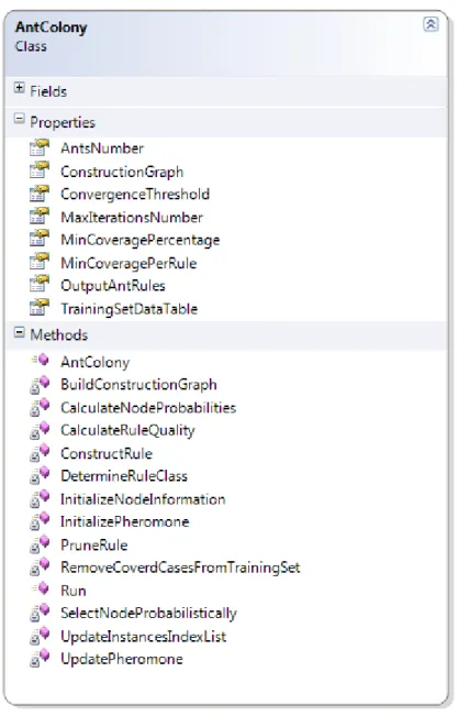
Figure ‎3.1 - AntColony Class Diagram. ... 66

Figure ‎4.1 - Construction Graph for AntMiner+. [18] ... 89

Figure ‎4.2 - A Path of an Ant in AntMiner+. [18] ... 90

(13)

xii

LIST OF ALGORITHMS

Algorithm ‎2.1 - Ant Colony Optimization Meta-heuristic. ... 18

Algorithm ‎3.1 - Original Ant-Miner. ... 44

Algorithm ‎4.1 - Ant_Miner3 State Transition Rule. ... 75

Algorithm ‎4.2 - Rule Pruning Procedure of the Original Version of Ant-Miner. ... 77

Algorithm ‎4.3 - Hybrid Rule Pruning Procedure. ... 78

Algorithm ‎4.4 - Multi-Label Ant-Miner (MuLAM). ... 81

Algorithm ‎4.5 - Unordered Rule Set Ant-Miner. ... 85

Algorithm ‎6.1 - Ant-Miner with Stubborn Ants. ... 105

(14)

xiii

LIST OF TABLES

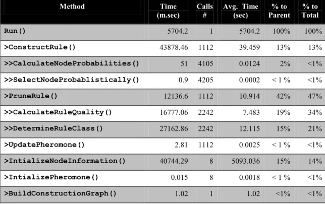
Table ‎3.1 - Ant-Miner Execution Profile. ... 70

Table ‎5.1 - Ant-Miner with Logical Negation Execution Profile. ... 101

Table ‎6.1 - Stubborn Ants Excution Profile. ... 111

Table ‎7.1 - Multi-pheromone Ant-Miner Execution Profile. ... 133

Table ‎8.1 - Ants with Personality Execution Profile. ... 140

Table ‎9.1 - Description of Dataset Used in the Experiments ... 143

Table ‎9.2 - Car Evaluation Dataset Experimental Results Summary ... 147

Table ‎9.3 - Car Evaluation Dataset Detailed Results for ANOVA Test ... 148

Table ‎9.4 - Tic-Tac-To Dataset Experimental Results Summary ... 149

Table ‎9.5 - Tic-Tac-To Dataset Detailed Results for ANOVA Test ... 150

Table ‎9.6 - Mushrooms Dataset Experimental Results Summary ... 151

Table ‎9.7 - Mushrooms Dataset Detailed Results for ANOVA Test ... 152

Table ‎9.8 - Nursery Dataset Experimental Results Summary ... 153

Table ‎9.9 - Nursery Dataset Detailed Results for ANOVA Test ... 154

Table ‎9.10 - Dermatology Dataset Experimental Results Summary ... 155

Table ‎9.11 - Dermatology Dataset Detailed Results for ANOVA Test ... 156

Table ‎9.12 - Soybean Dataset Experimental Results Summary ... 157

Table ‎9.13 - Soybean Dataset Detailed Results for ANOVA Test ... 158

Table ‎9.14 - Contraceptive Method Choice Dataset Experimental Results Summary . 159 Table ‎9.15 - Contraceptive Method Choice Dataset Detailed Results for ANOVA Test160 Table ‎9.16 - BDS Dataset Experimental Results Summary ... 161

Table ‎9.17 - BDS Dataset Detailed Results for ANOVA Test ... 162

(15)

1

Chapter 1

INTRODUCTION

1.1

Overview

Swarm intelligence is a branch of soft computing in which the biological collective behavior is applied [2]. Many animal groups, such as fish schools and bird flocks exhibit such a swarm behavior. This behavior can also be seen in insects like ants and bees that display structural order and integrated behavior (see figure 1.2). At a high-level, a swarm can be viewed as a group of homogenous agents cooperating in some purposeful behavior to achieve some goal. This collective intelligence seems to emerge from what are often large groups of relatively simple agents. The agents use simple local rules to govern their actions and via the interactions of the entire group, the swarm achieves its objectives. A type of self-organization emerges from the continuing actions of the group.

(16)

2

Since the early 90‘s, several collective behavior (like social insects, bird flocking) inspired algorithms have been proposed and applied studied optimization problems like NP-hard problems (Traveling Salesman Problem, Quadratic Assignment Problem, Graph problems), network routing, clustering, data mining, job scheduling and many other areas in order to solve problems that are combinatorial in nature.

Particle Swarm Optimization (PSO) and Ant Colonies Optimization (ACO) are the most popular algorithms in the swarm intelligence domain. PSO is a population-based search algorithm and is initialized with a population of random solutions, called particles [2]. Unlike in the other evolutionary computation techniques, each particle in PSO is also associated with a velocity. Particles move through the search space with velocities which are dynamically adjusted according to their historical behaviors. Therefore, the particles have the tendency to move towards better search areas over the course of search process. The following figure describes the basic structure for PSO algorithms.

(17)

3

Ant Colonies Optimization (ACO) algorithms were introduced around 1990 [8], [9], [10], [12]. These algorithms were inspired by the behavior of ant colonies. Ants are social insects, living in colonies and exhibit an effective collective behavior. Although each ant is relatively a simple insect with limited individual abilities, a swarm of ants has the ability to find the shortest path from their nest to food. This idea was the source of the proposed algorithms.

When searching for food, ants initially explore the area surrounding their nest in a random manner. While moving, ants leave a chemical pheromone trail on the ground. Ants are guided by pheromone smell. Ants tend to choose the paths marked by the strongest pheromone concentration. When an ant finds a food source, it evaluates the quantity and the quality of the food and carries some of it back to the nest. During the return trip, the quantity of pheromone that an ant leaves on the ground may depend on the quantity and quality of the food. The pheromone trails will guide other ants to the food source. The indirect communication between the ants via pheromone trails enables them to find shortest paths between their nest and food sources. As given by Dorigo et al. [13], the main steps of the ACO algorithm are given below:

1. Pheromone trail initialization.

2. Solution construction using pheromone. 3. State transition rule.

4. Pheromone trail update.

This process is iterated until a termination condition is reached. More details on the ACO algorithm are discussed in Chapter 3.

One of the most important application of swarm intelligence algorithms is data mining. Data mining is the application of specific algorithms for extracting patterns from

(18)

4

data. The additional steps in the Knowledge Discovery and Data mining process (KDD), such as data selection, data cleaning, and proper display and interpretation of the results are essential to ensure that useful knowledge is derived from the data.

The task of interest here is classification, which is the task of assigning a data point (a case in given a dataset) to a predefined class or group according to its predictive attributes. The classification problem and accompanying data mining techniques are relevant in a wide variety of domains such as financial engineering, medical diagnostic and marketing. The result of a classification technique is a model which makes it possible to classify future cases (in other words, predict the class of a new case) based on a set of specific attributes in an automated way, with a sufficient level of confidence.

In the literature, there is a lot of different techniques proposed for this classification task, some of the most commonly used being C4.5-based decision trees, logistic regression, linear and quadratic discriminate analysis, k-nearest neighbor, artificial neural networks and support vector machines. The performance of the classifier is typically determined by its predictive accuracy on an independent test set. Benchmarking studies have shown that the non-linear classifier generated by neural networks and support vector machines score best on this performance measure. However, comprehensibility can be a key requirement as well, demanding that the user can interpret the model to understand the motivations behind the model‘s prediction.

In some domains, such as credit scoring and medical diagnostics, the lack of comprehensibility is a major issue and causes a reluctance to use the classifier or even complete rejection of the model. In a credit scoring context, when credit has been denied the Equal Credit Opportunity Act of the U.S. requires that the financial institution

(19)

5

provides specific reasons why the customer‘s application was rejected, whereby vague reasons for denial are illegal. In the medical diagnostic domain as well, clarity and explainability are major constraints besides the classifier efficiency. The most suited classifiers for this type of problem are of course rules and trees. C4.5 is one of the techniques that construct such comprehensible, user-interpretable classification model with efficient predictive accuracy. On the other hand, other techniques, such as artificial neural network and support vector machine classifiers, are known for their predictive accuracy. However, they do not produce a comprehensive, explainable output.

Ant-Miner is an ACO algorithm, proposed by Parpinelli et al. [20], that discovers classification rules of the form:

IF <Term-1> AND <Term-2> AND . . . <Term-n> THEN <Class>

where each term is of the form <attribute = value>, and the consequent of a rule is the predicted class. Chapter 3 is dedicated to describe the Ant-Miner algorithm in detail, where its related work is discussed in Chapter 4.

1.2

Motivation

Ant-Miner performance was compared with the performance of the well-known C4.5 algorithm in six public domain data sets [26]. Overall the results show that, concerning predictive accuracy, Miner is competitive with C4.5. In addition, Ant-Miner has consistently found considerably simpler (smaller) rules than C4.5. Although applying ACO in the field of classification rule discovery was a new trend, Ant-Miner produced promising results compared to a well-known, sophisticated decision tree algorithm, which has been evolving from early decision tree algorithms for at least a couple of decades. This has motivated a lot of research to focus on such an algorithm.

(20)

6

Since the birth of this ACO-based classification algorithm, several ideas and modification have been applied to the original Ant-Miner version in order to enhance its performance, yet various enhancements and extensions can be investigated, tried and tested to develop Ant-Miner from the perspective of a classification algorithm. From another perspective, as an ACO-based technique, a lot of ACO-based ideas and updates that arise in the literature of swarm intelligence can be easily applied to the Ant-Miner algorithm.

1.3

Thesis Statement and Objective

According to the state of Ant-Miner as a new, promising classification rule discovery technique and its ACO-based algorithm nature, my objective is to:

“Implement effective extensions to the original version of Ant-Miner in order to improve its performance in terms of1) Produced model comprehensibility, via reducing the number of generated rules resulting in a smaller (simpler) model, 2) algorithm running time, via decreasing the number of iterations and the trials performed per iteration, and 3) produced model efficiency, via elevating the predictive accuracy of the generated rule set.”

1.4

Thesis Contribution

The main contribution of this Master‘s thesis consists of five extensions on the original Ant-Miner algorithm:

1. Logical Negation Operator: this allows the usage of a logical negation operator in the antecedents of constructed rules, so that the constructed rules would have a higher coverage. This should decrease the number of the generated rules, thus improving output comprehensibility, as well as increasing its classification accuracy.

(21)

7

2. Applying Stubborn Ants: an ACO-variation in which an ant is allowed to take into consideration its own personal history. The technique was introduced in 2008 in [1]. The idea is to promote search diversity by having each ant be influenced by its own history of constructing solutions in addition to the pheromone trails left by other ants. This tends to reduce the number of trials needed to converge on a rule per iteration. Besides, stubborn ants produce better results in terms of classification accuracy.

3. Multi-Pheromone Ant-Miner: using multiple types of pheromone, one for each permitted rule class, i.e. an ant would first select the rule class and then deposit the corresponding type of pheromone. An ant is only influenced by the amount of the pheromone deposited for the class for which it is trying to construct a rule. In this case, pheromone is not shared amongst ants constructing rules for different classes. This allows choosing terms that are only relevant to the selected class. This improves the classification accuracy of the generated rules.

4. Quality Contrast Intensifier: A new pheromone updates procedure where a rule whose quality is higher than a specific threshold would be rewarded by allowing it to deposit higher quantities of pheromone. In the same manner, rules with lower levels of quality are penalized by removing pheromone from their terms in the construction graph. This is used to direct the ants to use the good tried paths and unexplored paths rather than the low-quality-tried paths. The result of such an extension is to reduce the trials per rule and find better classification rules in term of accuracy. Moreover, a new convergence test is applied in order to insure that the discovered rule satisfies a minimum quality threshold. Otherwise, new different rules should be sought.

5. Ants with Personality: we allow each ant to have its own value of α and β parameters, which represent the weight of the cognitive component and the social

(22)

8

component respectively in the state transition formula (see formula 2.2). This in a sense means that each ant has its own individual personality. This promotes search diversity and helps in finding new better solutions.

1.5

Thesis Overview

This thesis is structured as follows:

Chapter 2 consists of two parts. Part1 describes the Ant Colony Optimization (ACO) technique in detail. It starts by explaining the biological behavior of the swarms, and then it moves to the artificial collective behavior and ACO meta-heuristic algorithm. Some ACO variations are discussed in the end of the chapter. The second part of Chapter 2 talks about data mining and knowledge discovery. Knowledge discovery steps are explained, followed by discussion of various data mining tasks. Challenges of data mining are tackled and different applications of data mining are mentioned at the end of this chapter.

Chapter 3 introduces the original version of Ant-Miner algorithm. A detailed description of the algorithm steps, results and algorithm issues are tackled in this chapter as well.

Chapter 4 exhibits some of the most important related work to the original version of Ant-Miner.

Chapter 5 to Chapter 8 introduce the extensions that have been applied on the original version of the Ant-Miner algorithm in the following order: Chapter 5 explains the use of logical negation operator in rule construction, Chapter 6 describes the use stubborn ants, Chapter 7 explains multi-pheromone system, applying a quality contrast intensifier

(23)

9

in pheromone update as well as introducing the new convergence test, and Chapter 8 shows the use of ants with personality.

Chapter 9 describes the experimental approach that was used to test the performance of the new modifications on the algorithm. Experimental results and their discussion are shown in this chapter as well.

(24)

10

Chapter 2

BACKGROUND

PART 1: ANT COLONY OPTIMIZATION

2.1

Introduction to ACO

Ant Colony Optimization (ACO) is subfield of swarm intelligence which studies algorithms inspired by the observation of the behavior of biological ant colonies. ACO was proposed by M. Dorigo et al. [8 – 9] as meta-heuristic method for solving optimization problems. As was described in Chapter 1, swarm intelligence algorithms are self-organizing systems that are made up of simple individuals cooperating with each other to achieve a goal, without any form of central control over the swarm members. Although ants are simple insects, ant colonies are able to solve complex problems such as finding shorts path from the nest to the food utilizing the collective behavior of the whole swarm communicating indirectly with each other via pheromone trails. This chapter illustrates the basic ideas of ACO and describes some variations in the literature for the algorithm. A comprehensive overview about ACO can be found in ―Ant Colony Optimization‖, a book by M. Dorigo and T. Stützle [13].

2.2

Biological Ants Behavior

Social insect swarms like ant colonies are distributed systems that, in spite of the simplicity of their individuals, produce a collective behavior that enables a swarm of insects to accomplish complex tasks that, in some cases, far exceed the individual capabilities of a single insect [13]. The high coordinated, self-organizing structure that is exhibited by colonies of ants can be used to build an agent-based artificial system to solve

(25)

11

hard computational problems. Ants coordinate their activities via stigmergy, a form of indirect communication mediated by altering the environment.

As an example of stigmergy observed in colonies of ants, an ant drops a chemical substance called a pheromone while waking from source to food and vice versa. Other ants are able to smell this pheromone, and its presence influences the choices they make along their path. An ant is more likely to follow route containing high concentrations of pheromone over one that does not. The pheromone deposited on the ground forms a pheromone trail, which allows the ants to find good sources of food that have been previously identified by other ants. The similar types of behavior of ant colonies have inspired different kinds of ant algorithms, foraging, division of labor, brood sorting, and cooperative transport.

The ―double bridge‖ is an effective experiment was done by Deneubourg et al. in the 90s [6] to explore the pheromone trail-laying and -following behavior of Argentine ant species. The experiment shows the collective behavior of ants that emerges through pheromone trial-based communication, which leads to converge on the shorter path from source to distention. The following section presents an overview of this experiment.

2.2.1Double Bridge Experiment

The nest of the ants was connected to a food source by two bridges. In the first experiment, the two bridges were equal in length. The behavior of the ants in choosing which branch to take when searching for food and bringing it back to the nest was then observed over time. The ants start exploring the surroundings of the nest and randomly find one of the bridges and reach the food source. During their journey to the food source and back, the ants deposit pheromone on the bridge that they use. Initially, each ant

(26)

12

randomly chooses one of the bridges. After some time, there will be more pheromone deposited on one of the bridges than on the other. Because ants tend to prefer in probability to follow a stronger pheromone trail, the bridge that has more pheromone will attract more ants. This in turn makes the pheromone trail grow stronger, until the colony of ants converges toward the use of a same bridge.

In another experiment, the two bridges were not of the same length so that the longer branch was twice as long as the short one. At the beginning, ants leave the nest to explore the environment and arrive at a decision point where they have to choose one of the two branches. The two branches initially appear identical to the ants, they choose randomly. Therefore, it can be expected that, on average, half of the ants choose the short branch and the other half the longer branch. Because one branch is shorter than the other, the ants choosing the short branch are the first to reach the food and to start their return to the nest. Therefore, the pheromone intensity will increase faster on the short branch. Then, when other ants make a decision between the two bridges, the higher level of pheromone on the short branch will bias their decision in its favor, which will in time be used by all the ants because of the autocatalytic process described previously.

Figure 2.1 - Experimental Setup for the Double Bridge Experiment. [6] (a) Branches have equal length. (b) Branches have different length.

(27)

13

Figure 2.2 - Traffic Behavior for each Case in the Double Bridge Experiment. [6] (a) Branches have equal length. (b) Branches have different length.

When compared to the experiment with the two branches of equal length, the influence of initial random fluctuations is much reduced, and stigmergy, autocatalysis, and differential path length are the main mechanisms at work. Interestingly, it can be observed that, even when the longer branch is twice as long as the short one, not all the ants use the short branch, but a small percentage may take the longer one. This may be interpreted as a type of ‗‗path exploration.‘‘ Figure 2.1 and 2.2 show the experimental setup and observed result for both experiments. Figures were taken from [13].

2.2.2Related Algorithmic Model

A model was developed by Goss et al. [7] to explain the behavior observed in the double bridge experiment described in the previous section. As explained in [13], assuming that number of ants has taken the first branch and has taken the second one after unites of time. The probability that ant selects the first branch is given by the following equation:

(28)

14

where parameters and are needed to fit the model to the experimental data. The probability that the same ant chooses the second bridge is 1- . This model assumes that the amount of pheromone on a branch is proportional to the number of ants that used the branch in the past and no pheromone evaporation is considered by the model. So the at any given time , the probability that that an ant chooses branch depends on the number of ants that have previously selected that branch. Assuming that branch is the shorter one. At time the number of ant that has taken branch is probably larger as they take the path from the nest to the food and back in a shorter amount of time than the other branches. Therefore, the probability of ant to select the shorter branch would be larger than the probability of selecting other branches.

This basic model explains the foraging behavior of real ants in solving such an optimization problem, which is finding the shortest path, without any global sight or master control. Instead, stigmergic communication happens via the pheromone that ants deposit on the ground. This can be an inspiration to design artificial ants that solve optimization problems defined in a similar way. The following section describes ideas behind artificial ants.

2.2.3Artificial Ants

The binary bridge experiments show that ant colonies exhibit a collective behavior that is able to solve optimization problems. With stigmergic communication, via pheromone depositing and the use of probabilistic rules based on local information they can find the shortest path between two points in their environment. An idea towards an artificial ant system is to represent the solution space for any optimization problem as a

(29)

15

set of nodes in a graph, representing the variable states of the solution. Artificial ants can visit these states to build a candidate solution for the problem. Artificial ants may simulate pheromone laying by modifying an appropriate pheromone variable associated with solution states they visit. They would have only local access to these pheromone variables according to the stigmergic communication model.

Ant Colony Optimization (ACO) is an artificial ants system that basically follows the previously described ideas of real ants' behavior. Both real and artificial ant colonies are composed of a swarm of simple individuals that use collective behavior to achieve a certain goal. In the case of real ants, the goal is to find the food using a good (short) path, while in the case of artificial ants, it is to find a good solution to a given optimization problem. A single ant (either a real or an artificial one) is able to find a solution to its problem, but only cooperation among many individuals through stigmergy enables them to find good solutions.

Artificial ants live in a virtual world, probably a graph of nodes representing the search space of the solution for a given problem. The use of pheromone, which is in the artificial system a numeric variable associated with each state in the search graph, depositing and influenced by it while searching in the solution states graph constructing a solution. A sequence of pheromone values associated with problem states is called artificial pheromone trail.

There are many similarities between real and artificial ants. However, there are some important differences between real and artificial ants. These differences are listed below as were described by M. Dorigo and T. Stützle in [13]:

 Artificial ants live in a discrete world—they move sequentially through a finite set of problem states.

(30)

16

 In real ants, there is the coupling between the autocatalytic mechanism and the implicit evaluation of solutions. As for the double bridge experiment, the fact that shorter paths are completed earlier than longer ones, and therefore they receive pheromone reinforcement quicker. So the shorter the path is, the sooner the pheromone is deposited, and the more the ants use the shorter path. On the other hand, artificial ants drop pheromone after the solution is constructed and its quality is evaluated. This may not have anything related to the quickness in which the pheromone accumulates on a path due to its length. Thus, the amount of the pheromone may vary according to the quality of the solution to simulate enforced catalytic mechanism toward the good paths.

 Artificial ants may use local heuristics, local search and other additional mechanisms. The following section describes ant colony optimization meta-heuristic model in detail with illustration of the ACO algorithm.

2.3

Ant Colony Optimization Meta-Heuristic

“A meta-heuristic refers to a master strategy that guides and modifies other heuristics to produce solutions beyond those that are normally generated in a quest for local optimality.” —Tabu Search, Fred Glover and Manuel Laguna, 1998.

In other words, meta-heuristic it is a set of algorithmic concepts that can be used to define heuristic methods applicable to a wide set of different problems [13]. This can be seen as a general-purpose method designed to guide an underlying problem-specific heuristic toward promising regions of the search space containing high-quality solutions. A meta-heuristic is therefore a general algorithmic framework which can be applied to

(31)

17

different optimization problems with relatively few modifications to make them adapted to a specific problem.

M. Dorigo et al. formalized an ACO meta-heuristic model using pheromone manipulation for solving Combinational Optimization Problems (COPs) [8]. This has since been used to tackle many combinatorial optimization problems. The model can be defined as follows; a model of a COP consists of:

 A search space defined over a finite set of discrete decision variables and a set of constraints among the variables.

 An objective function to be optimized (minimized or maximized).

The search space is a set of discrete variables , with discrete values . A variable instantiation is the assignment of value to variable , denoted by . An instantiated decision variable is called a solution component and denoted by , The set of all possible solution components is denoted by .Any solution , that is a complete variables assignment in which each decision variable has a value assigned that satisfies all the constraints in the set , is a feasible solution of the given COP. A solution is called a global optimum if and only if (for minimization). The set of all globally optimal solutions is denoted by . To solve a (COP), at least one needed to be found.

The aforementioned model for COP is the basis for pheromone manipulation used in ACO. A pheromone trail parameter is associated with each component . The set of all pheromone trail parameters is denoted by . The value of a pheromone trail parameter in a given time associated with decision component is denoted by . This pheromone value is then used and updated by the (ACO) algorithm during the

(32)

18

search. This allows modeling the probability distribution of different components of the solution.

In ACO, the described model is represented as a graph, called construction graph, which is traversed by artificial ants to build a solution for a given problem. The construction graph is a fully connected graph consisting of a set of vertices and a set of edges . The set of components may be associated either with the set of vertices of the graph , or with the set of its edges . An ant constructs a solution incrementally while moving from vertex to vertex along the edges of the graph. Additionally, the ant deposits a certain amount of pheromone on the components, that is, either on the vertices or on the edges that they visit. The amount of pheromone, , deposited depends on the quality of the solution found. Subsequent ants are influenced by pheromone trails and use them as guides toward good decision components in the search graph. This increases the probability of choosing such decision components in the following ant trials. The ant colony optimization meta-heuristic technique is shown in the following algorithm.

Algorithm 2.1 - Ant Colony Optimization Meta-heuristic. Set parameters, initialize pheromone trails.

WHILE termination conditions not met

DO

Construct a Solution

Apply Local Search {optional} Update Pheromone

(33)

19

As shown in Algorithm 2.1, each ant in the swarm builds a solution by incrementally selecting solution components from the construction graph utilizing the pheromone on it. A local search might be applied to enhance the solution quality. Then the pheromone is updated on the ant trail during its navigation. The amount of pheromone to deposit may depend on an evaluation function used to determine the quality of the constructed solution. These steps are repeated until a predefined termination condition is met. The following is a more detailed explanation for the basic components of the algorithm.

2.3.1Construct a Solution

Each constructs a solution from elements of a finite set of available solution components in the construction graph , where represents the index of the solution variable and the index of the value belonging to the domain this variable. Each starts with an empty solution . At each step in the solution construction, a valid solution component is added to the partial solution from a set of feasible neighbors to the current ant solution state . The process of constructing a solution can be viewed as a path in the construction graph where the set of constraints among the variables defines the feasible neighbors at each step according to the current state of the partial solution .

The decision component selection at each step is done probabilistically according to the following formula:

(34)

20

(2.2)

where:

 is the amount of the pheromone associated to component at time .  is a problem dependent heuristic value assigned to component .

 and are positive parameters, whose values determine the relative importance of pheromone versus heuristic information.

2.3.2Apply Local Search

Local search is an optional solution that can be applied after the solution is constructed in order to enhance the solution by locally optimizing it. Local search a can be implemented as problem specific operation and is done before the pheromone update step. Then the locally optimized solutions are then used to decide which pheromones to update. Local search improves the quality of the solution constructed and enhances the overall output of the algorithm. However, it might be an expensive operation depending on the combinations scope that the operation searches in. Local search can be done after each ant constructs a solution or can be done iteration based on the best solution constructed by set of ants per iteration.

2.3.3Update Pheromone

After a solution is constructed, the pheromone on the construction graph is updated to guide subsequent ants to good decisions to take while constructing their solutions. This pheromone update is done by two steps:

 Pheromone Reinforcement: this done by increasing the pheromone value associated

(35)

21

solution, as they are good or promising components. The reinforcement is done by the following equation:

(2.3) where is a fitness function that evaluates the quality of solution .

 Pheromone Evaporation: this is done by decreasing the pheromone value associated with all in the construction graph so that the bad components (the ones that are not being chosen frequently) get their pheromone values decreased and give space to other components in unexplored regions in the construction graph to get selected. This is to avoid early convergence of the algorithm. Evaporation is done as follows [13]:

(2.4) where is evaporation factor parameter .

2.4

Traveling Sales Person Problem

This section describes the implementation of ACO and how it works to solve the famous NP-hard problem: traveling sales person. The TSP consists of a set of locations (cities) and a traveling salesman that has to visit all the locations once and only once. The distances between the locations are given and the task is to find a Hamiltonian tour of minimal length.

(36)

22

Figure 2.3 - Construction Graph for TSP with Four Cities.

The first thing to apply ACO on a problem is to have a construction graph that represents the solution components space for the problem. As shown in figure 2.3, the construction graph for TSP consists of vertices representing the cities

. is the set of edges connecting the cities, which represents the solution components , and with which the pheromone is associated. The length value of each edge represents the distance between city and .

Each ant starts from a randomly selected location (vertex of the graph ). Then, at each construction step it moves along the edges of the graph, by which it selects a solution component. Each ant memorizes the solution components (edges) that it selected through its path, and in subsequent steps it chooses among the edges that do not lead to vertices that it has already visited (this constraint defines feasible movements to the ant according to its current partial solution ) . At each construction step an ant chooses probabilistically the edge to follow using equation (2.2). An ant has constructed a solution once it has visited all the vertices of the graph.

Afterwards, the pheromone is updated according to the quality of the constructed path. A possible fitness function for TSP solution is:

(2.5)

which is the inverse of the length of the tour constructed by the ant. Ant colony optimization has been shown to perform quite well on the TSP [25].

(37)

23

2.5

ACO Variations

2.5.1Ants System

Ant System was introduced in the literature by M. Dorigo et al. in [9]. It is the first ACO algorithm to be proposed. Its main characteristic is that the pheromone values are updated by all the ants that have completed constructing the solution. In other words, after each ant constructs a solution, it updates its pheromone trial according to the quality of the solution it generated, unlike other techniques which update the pheromone after the best solution is selected among a set of ants that constructed solution in an iteration of the algorithm.

2.5.2MAX-MIN Ant System

MAX -MIN Ant System is an improvement over the original Ant System idea. MMAS was proposed by T. Stützle and Hoos in [24], who introduced a number of changes of which the most important are the following: only the best ant can update the pheromone trails, and the minimum and maximum values of the pheromone are limited.

2.5.3Ant Colony System

Another improvement over the original Ant System is Ant Colony System (ACS), introduced by L. M. Gambardella and M. Dorigo [11]. The most interesting contribution of ACS is the introduction of a local pheromone update in addition to the pheromone update performed at the end of the construction process (offline pheromone update). The main goal of the local update is to diversify the search performed by subsequent ants during the same iteration. In fact, decreasing the pheromone concentration on the edges as they are traversed during one iteration encourages subsequent ants to choose other edges

(38)

24

and hence to produce different solutions. This makes the possibility of several ants producing identical solutions per a given iteration less likely.

PART 2: DATA MINING AND KNOWLEDG DISCOVERY

2.6

Introduction to Data Mining

Since the widespread of transactional software that has automated various systems in different fields, a huge volume and variety of data has been continuously collected. Storing and retaining immense amounts of data in easily accessible form was availed effectively. As a matter of fact, this raw data potentially stores a huge amount of information and hidden patterns. Hence, the need of discovering these hidden patterns and convert them into useful knowledge arose.

The notion of finding useful patterns in data has been given a variety of names including data mining, knowledge extraction, information discovery, and data pattern processing. Data mining is the application of specific algorithms for extracting patterns from data. Research directions have emerged in the recent past for tackling the problem of making sense out of large, complex data sets. As conventional methods for sifting through huge amounts of data manually and making sense out of it is slow, expensive, subjective and prone to errors, the need to automate the process has been a research focus. Knowledge discovery from databases (KDD) evolved as a research with multi-disciplinary fields containing databases, machine learning, pattern recognition, statistics and artificial intelligence.

Data is stored in huge repositories with high dimensionality in different types and formats; numerical, textual, graphical, symbolic, linked. Typical examples of some such domains are the world-wide web, geo-scientific data, maps, multimedia, and time series

(39)

25

data as in financial markets. In addition, the type of the knowledge wished to be discovered varies in a wide range according to the domain of interest and it task of use needed from the knowledge. All these factors encourage developing advanced techniques for mining complex data.

2.7

Knowledge Discovery Steps

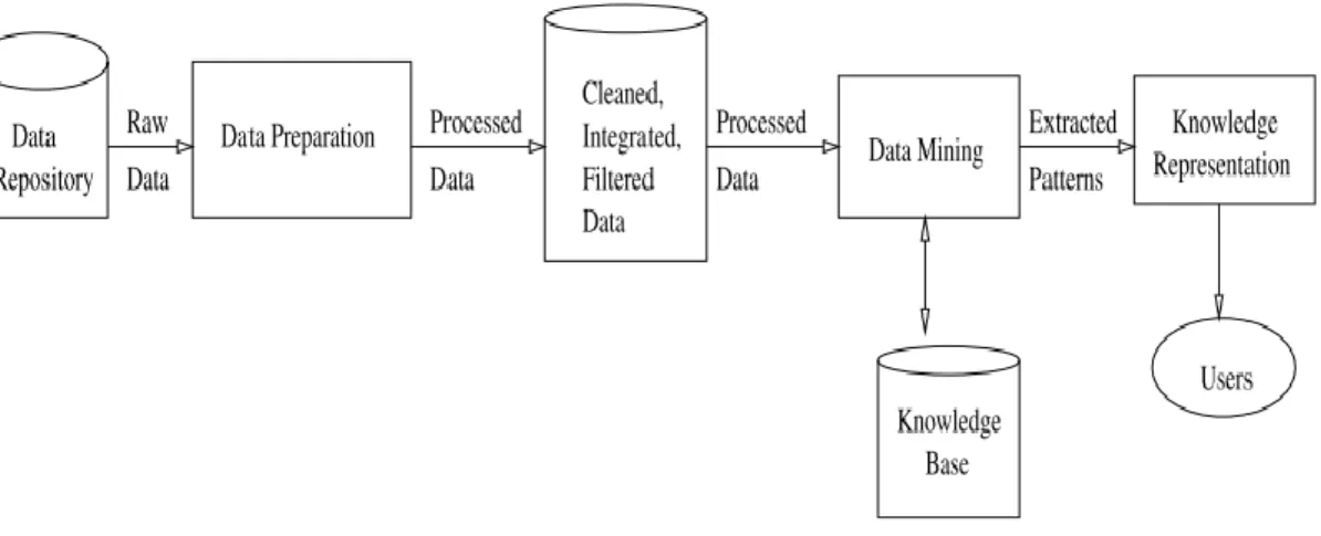
Basically, Knowledge discovery process has three essential parts: data preparation, data mining and knowledge presentation. Data mining is the core step where the techniques for extracting the useful hidden patterns are applied. In this sense, data preparation and knowledge presentation can be considered, respectively, to be pre-processing and post-pre-processing steps of data mining.

Figure 2.4 - Knowledge Discovery Process.

As shown in Figure 2.4, raw data in different types and formats is received from non-homogenous data sources. Various tasks of data preparation and data fusion are applied to the raw data to create a cleansed, filtered, integrated and malleable version that is appropriate for different task of information retrieval and knowledge extraction. As data mining algorithms are applied, generated models and discovered knowledge are

(40)

26

stored in a knowledge base for further usage. A neat presentation and visualization is required for the knowledge to facilitate user interaction.

2.8

Data Preparation

Data source repositories have data in different types and formats. Some errors may occur during the data recording and storing by the source system such as missing values, noise, inconsistency etc. In addition, among the huge amount of the available data, only some parts of it can be interesting or useful for a specific knowledge discovery task and other parts should be neglected. Data needs different structures and formats to be suitable for data knowledge discovery processing tasks. Therefore, before going to perform mining on the data, some kind of pre-processing [15] is required. Preprocessing of data is done in the following major ways:

 Data cleaning: This is performed to remove inconsistency, noise to fill up missing values and to filter needed portions.

 Data integration. This is needed to combine and unify data from multiple different sources like databases, data cubes, flat files etc. Correlation analysis, detecting data conflict, and resolving semantic heterogeneity are used for data fusion.

 Data transformation. The format of data in the repositories may not be suitable for processing. So, the format of the data should be transformed to a one suitable for a particular task. This is done for smoothing, aggregation, generalization, normalization, and attributes construction.

 Discretization. This step consists of transforming a continuous attribute into a categorical (or nominal) attribute, taking only a few discrete values - e.g., the real-valued attribute. Salary can be discretized to take on only three values, say "low",

(41)

27

―medium", and ―high". This step is particularly required when the data mining algorithm cannot cope with continuous attributes. In addition, discretization often improves the comprehensibility of the discovered knowledge.

 Data reduction. This is needed to have a reduced version of data that can work effectively with a data mining algorithm. This data reduction is done in terms of dimensionality reduction, data cube aggregation, as well as data compression.

 Data selection. For the purpose of processing and analysis, relevant data are selected and retrieved in this step.

2.8.1Data Mining

Data mining is the core part in the knowledge discovery process, which aims to discover and extract interesting, potentially useful hidden patterns from large amounts of data. Patterns discovered could be of different types such as associations, trees, profiles, sub-graphs, and anomalies. The interestingness and the usefulness of the knowledge to be discovered are relative to the problem and the concerned user. A piece of information may be of immense value to one user and absolutely useless to another. Often data mining and knowledge discovery are treated as synonymous, while there exists another school of thought which considers data mining to be an integral step in the process of knowledge discovery.

Different data mining techniques are used to carry out different knowledge discovery tasks. Classification, clustering, association analysis, regression and deviation detection are the most common data mining techniques that are used for different knowledge discovery task. These techniques are described in the following section.

(42)

28

Data mining techniques mostly consist of three components: a model, a preference criterion and a search algorithm [14]. The most common model functions in current data mining techniques include classification, clustering, regression, and link analysis and dependency modeling. A model is selected according to the intended discovery task and the nature of the useful knowledge to be extracted. Models vary in the flexibility of the model for representing the underlying data and the interpretability of the model in human terms. This includes decision trees and rules, linear and nonlinear models, example-based techniques such as NN-rule and case-based reasoning, probabilistic graphical dependency models (e.g., Bayesian network) and relational attribute models. The preference criterion is used to evaluate the efficiency of the model according the underlying dataset. Preference citation can determined which model to use for mining, as it best fits the current nature of data. It tries to avoid over-fitting of the underlying data or generating a model function with a large number of degrees of freedom. The search algorithm is then defined for the model that carries out the intended knowledge discovery task.

2.8.2Knowledge Presentation

As the knowledge is extracted, the user should be able to interpret this knowledge and make use of the extracted patterns for decision making concerning his domain. The discovered knowledge will be interesting for the user if it is easily understood, valid, novel and useful. Presentation of the information extracted in the data mining step in a format easily understood by the user is an important issue in knowledge discovery. Data visualization and knowledge representation are important components. The following are some interesting ways of data presentation:

(43)

29  Graphs.

 Tables and cross-tabs  Charts and Histograms.

 Natural language generated rules.

2.9

Overview of Data Mining Tasks

Data mining tasks vary according to what types of knowledge we are want to try and discover and how the discovered knowledge is intended to be used. In general, data mining tasks can be classified into two categories, descriptive and predictive [15]. The descriptive techniques provide a summary of the data and profile its general characteristics and properties. On the other hand, the predictive techniques learn from the current data in order to make forecasts or predictions about the behavior of new data. The following is description of most commonly used data mining tasks.

2.9.1Classification

Classification is a type of supervised learning. In supervised learning, the data set contains objects with several attributes as input features for each object, and one attribute is considered the class (or the label) of this object. Classification is a process of building a model that can describe and classify the object class as a function of its input attributes. As shown in figure 2.5, the input for classifier model discovery is a training set that contains labeled cases (cases which their classes are known). A classification model is built upon relationship patterns discovered between the input attributes and the classes of the cases. Now the classification model is able to classify (find the class) of unlabeled input cases, whether they are a testing set of cases or whole new cases which their classes need to be predicted.

(44)

30

Figure 2.5 - Process of Building a Classification Model.

Note that some data mining techniques for classification generate a classifier that can only classify unlabeled cases without describing the relationships between the attributes of a case and its class. Examples of such techniques are the nearest neighbor classifier, Bayes maximum likelihood classifier and Neural Networks-based classifier. Other techniques can produce a classification model that not only can predict a class of an unlabeled case, but can also describe the relationships between the input features and the classes of the cases. This description can be in the form of rules or classification trees. Decision trees and rule induction are examples. The latter type of classification techniques has an advantage of model interpretation as it provides insight for the user regarding the data at hand and on the relationship patterns amongst it. Some of these techniques are now briefly described.

 Nearest Neighbor Classifier: It assigns the unlabeled cases the class of the nearest neighbor to it within the labeled training set. Given a training set with many labeled cases , the distance is calculated between the new unlabeled case

(45)

31

and each case in the training set using distance function. The new unlabeled case is given the class of case that has the least value of distance with it. If k-nearest neighbor is considered, the new case is assigned the class of the majority of the nearest cases [15].

 Naïve Bayes Classifier: is a simple probabilistic classifier based on applying Bayes' theorem with attributes independence assumptions [15]. Let us consider having a data set with attributes for each case. Assuming that attributes are conditionally independent of one another given class , we have:

(2.6)

This is a dramatic reduction compared to the parameters needed to characterize if we make no conditional independence assumption. Naïve Bayes aims to train a classifier that will output the probability distribution over possible values of , for each new instance that we ask it to classify. The expression for the probability that will take on its k-th possible value is the maximum value of the following equation calculated for each :

(2.7)

 Decision Trees: A decision tree is an acyclic graph. In these tree structures, leaves represent classifications and branches represent conjunctions of features that lead to those classifications. It is easy to convert any decision tree into classification rules. Once the training data set is available, a decision tree can be constructed from them from top to bottom using a recursive divide and conquer algorithm. This process is

(46)

32

also known as decision tree induction. A version of ID3 [15], a well-known decision-tree induction algorithm, is described below.

1. Create a node N.

2. If all training data points belong to the same class (C)then return N as leaf node labeled with class C.

3. If cardinality (features) is NULL then return N as a leaf node with the class label of the majority of the points in the training data set.

4. Select a feature (F) corresponding to the highest information gain, then label node

N with feature F.

5. For each known value of F, partition the data points as . 6. Generate a branch from node N with the condition feature = .

7. If is empty, then attach a leaf labeled with the most common class in the data points left in the training set.

8. Else attach the node returned by Decision tree induction ( , (features-F)).

Assume we have a data set with cases labeled with classes. is the number of cases belonging to class . Suppose that each case has features

. Each feature F can the cases into subsets . The information gain of a feature is measured by the following equation:

(2.8) where (2.9) and

(47)

33

(2.10)

Here, is the probability that a data point in belongs to class .

2.9.2Clustering

Clustering is the process of partitioning the input data set into groups or segments, where each group is called a cluster. Each cluster contains a subset of the data points that are more similar to one another and less similar (dissimilar) to data points in other clusters. The similarity and dissimilarity are measured in terms of some distance function. Cluster analysis serves as a powerful descriptive model that can profile the data point according to its attributes and exhibits similarities and dissimilarities between the data clusters that are found.

Clustering is considered as an unsupervised learning, as the input cases to any clustering technique are not required to be labeled. The clustering algorithm should discover these labels as each cluster can be considered as a class for the data points that it contains after it is discovered.

K-Means algorithm [15] has been one of the more widely used ones; it consists of the following steps:

1. Choose initial cluster center , ,.., randomly from the domain space of the input data point .

2. Assign each data point to cluster , if the distance between and is the least among the distance between and all other cluster centers.

(48)

34

_(2.11)

where is the number of data points belonging to cluster .

4. Terminate if no change in the centers occurs or upon meeting any other criteria. Although K-means is one of the widely used clustering algorithms, it suffers from shortcomings. Outliers can affect the computation of centriods. K-medoid attempts to alleviate this problem by using the medoid, the most centrally located object, as the representative of the cluster. (PAM), (CLARA) and (CLARANS) are various implementations of K-medoid. Fuzzy K-Means cluster the data set with membership value associated with each data point for each cluster. Hierarchal clustering uses top down (divisive) or bottom up (aggregative) approach to find clusters with no initial cluster center and now initial clusters number. Density based clustering (DBSCAN) is another clustering technique that can discover arbitrarily-shape clusters, which is used for mining spatial data. [15].

2.9.3Association Rules Mining

Discovery of association relationship among large set of data items is useful in decision-making. A typical example for association rules mining is market basket analysis, which studies customer buying habits by finding associations between the different items that customers place in their baskets. An association rule is thus a relationship of the form: , where and are sets of items and . Such a rule generation technique consists of finding frequent item sets

(49)

35

from which rules like are generated. The measures support is the percentage of transactions that contain both the item sets. Thus:

(2.12)

(2.13)

Although both classification and association rules have an IF-THEN structure, association rules can have more than one item in the consequent part, whereas classification rules always have one attribute (class label) in the consequent. In other words, for classification rules, predicting attributes and the goal attribute. Predicting attributes can occur only in the rule antecedent, whereas the goal attribute occurs only in the rule consequent.

2.9.4 Regression

Regression analysis includes any techniques for modeling and analyzing several variables (criterion), when the focus is on the relationship between a dependent variable and one or more independent variables (predictor). More specifically, regression analysis helps us understand how the typical value of the dependent variable changes when any one of the independent variables is varied, while the other independent variables are held fixed.

Linear regression is a form of regression where the relationship between variables is modeled with a straight line (linear equation), learned using the training data points. A straight line, through the input vector (known as predictor variable) and the output vector (known as response variable), can be modeled as where and are the regression coefficient and slope of the line, computed as:

(50)

36 (2.12) (2.13)

where and are averages of