Time Series Classification with Artificial Neural Networks

(1)

doc. Ing. Jan Janoušek, Ph.D. Head of Department

prof. Ing. Pavel Tvrdík, CSc. Dean

CZECH TECHNICAL UNIVERSITY IN PRAGUE

FACULTY OF INFORMATION TECHNOLOGY

ASSIGNMENT OF MASTER’S THESIS

Title: Time Series Classification with Artificial Neural Networks Student: Bc. Jakub Waller

Supervisor: Ing. Tomáš Borovička Study Programme: Informatics

Study Branch: Knowledge Engineering

Department: Department of Theoretical Computer Science Validity: Until the end of summer semester 2017/18

Instructions

Artificial Neural Networks are often used for time series modeling and classification. In the last decade, advanced architectures such as deep neural networks or neural networks with memory became popular, because computational power is more widely available. Convolutional neural networks or long-short term memory networks are examples successfully applied on time series modeling and classification.

1) Review and theoretically describe different state-of-the-art ANN architectures suitable for univariate as well as multivariate time series classification.

2) Propose an experiment design in order to compare their ability to learn, effectivity of the training process and classification performance.

3) Compare different architectures on a set of benchmark datasets.

References

(2)

(3)

Czech Technical University in Prague Faculty of Information Technology

Department of Theoretical Computer Science

Master’s thesis

Time Series Classification with Artificial

Neural Networks

Bc. Jakub Wal ler

Supervisor: Ing. Tom´aˇs Boroviˇcka

(4)

(5)

Acknowledgements

I would like to thank my supervisor Ing. Tom´aˇs Boroviˇcka for his valuable advice and inspiring guidance. I am also very grateful to the Data Science Laboratory at CTU FIT and Datamole for their support. Finally, I wish to thank all precious people close to me.

(6)

(7)

Declaration

I hereby declare that the presented thesis is my own work and that I have cited all sources of information in accordance with the Guideline for adhering to ethical principles when elaborating an academic final thesis.

I acknowledge that my thesis is subject to the rights and obligations stip-ulated by the Act No. 121/2000 Coll., the Copyright Act, as amended. In accordance with Article 46(6) of the Act, I hereby grant a nonexclusive author-ization (license) to utilize this thesis, including any and all computer programs incorporated therein or attached thereto and all corresponding documentation (hereinafter collectively referred to as the “Work”), to any and all persons that wish to utilize the Work. Such persons are entitled to use the Work in any way (including for-profit purposes) that does not detract from its value. This authorization is not limited in terms of time, location and quantity. However, all persons that makes use of the above license shall be obliged to grant a license at least in the same scope as defined above with respect to each and every work that is created (wholly or in part) based on the Work, by modi-fying the Work, by combining the Work with another work, by including the Work in a collection of works or by adapting the Work (including translation), and at the same time make available the source code of such work at least in a way and scope that are comparable to the way and scope in which the source code of the Work is made available.

(8)

Czech Technical University in Prague Faculty of Information Technology

c

This thesis is school work as defined by Copyright Act of the Czech Republic. It has been submitted at Czech Technical University in Prague, Faculty of Information Technology. The thesis is protected by the Copyright Act and its usage without author’s permission is prohibited (with exceptions defined by the Copyright Act).

Citation of this thesis

Waller, Jakub. Time Series Classification with Artificial Neural Networks. Master’s thesis. Czech Technical University in Prague, Faculty of Information Technology, 2017.

(9)

Abstrakt

Mnoho r˚uzných architektur umˇelých neuronových s´ıt´ı bylo navrˇzeno, kupˇ r´ıkla-du konvoluˇcn´ı neuronové s´ıtˇe a long short-term memory neuronové s´ıtˇe. C´ılem této práce je aplikovat tyto s´ıtˇe na klasifikaci ˇcasových ˇrad. Po teoretickém popisu tˇechto architektur je navrˇzena metoda pro jejich experimentáln´ı poro-vnán´ı, a ta je následnˇe implementována v Pythonu. Tato metoda zahrnuje automatickou optimalizaci hyperparametr˚u neuronových s´ıt´ı. Popsané ar-chitektury jsou poté d˚ukladnˇe porovnány na tˇrech benchmarkových data-setech. Toto porovnán´ı ukazuje, ˇze long short-term memory neuronové s´ıtˇe dosahuj´ı na dvou ze tˇr´ı dataset˚u lepˇs´ıch výsledk˚u neˇz konvoluˇcn´ı neuronové s´ıtˇe.

Kl´ıˇcová slova konvoluˇcn´ı neuronové s´ıtˇe, rekurentn´ı neuronové s´ıtˇe, long

short-term memory neuronové s´ıtˇe, hluboké uˇcen´ı, optimalizace hyperpara-metr˚u, grid search, random search, klasifikace ˇcasových ˇrad

(10)

Abstract

Various architectures of artificial neural networks have been developed such as convolutional neural networks and long short-term memory neural net-works. The aim of this thesis is to apply these networks on the classification of time series. After a theoretical description of the architectures, an ex-perimental procedure for their comparison is proposed and implemented in Python. The procedure includes automatic optimisation of neural network’s hyperparameters. Based on this procedure, the architectures are thoroughly compared on three benchmark data sets. The comparison shows that long short-term memory neural networks achieve better results than convolutional neural networks on two of these data sets.

Keywords convolutional neural networks, recurrent neural networks, long

short-term memory neural networks, deep learning, hyperparameters optim-isation, grid search, random search, time series classification

(11)

List of Figures

1.1 Structure of a simple 3-layer neural network. . . 4

1.2 Artificial neurone. . . 5

1.3 A simple network with two input nodes, one output neurone, and a node representing the error functionE. . . 7

1.4 Scheme of a convolutional neural network with B= 2, C = 2, and D= 1. . . 10

1.5 The processing of two regions by one filter of size three, with zero-padding equal to zero and stride equal to one. . . 11

1.6 Recurrent neural network unfolded into three time-steps with a se-quential output. . . 12

1.7 Recurrent neural network unfolded into three time-steps with a non-sequential output. . . 13

1.8 The sigmoid function and its derivative. . . 14

1.9 LSTM’s hidden unit. . . 15

1.10 Adding peephole connections to LSTM’s hidden unit. . . 17

3.1 A graphical schema of the experimental procedure. . . 25

3.2 An example of the Gun-Draw class from the Gun-Point data set. . 31

3.3 An example of the Point class from the Gun-Point data set. . . 31

3.4 An example of the Strawberry class from the Strawberry data set. 32 3.5 The Japanese Vowels data set. . . 33

3.6 The classification performance in dependency on the number of neurones and the number of layers for CNN on the Gun-Point data set. . . 35

3.7 The classification performance in dependency on the number of neurones and the number of layers for LSTM on the Gun-Point data set. . . 35

3.8 The classification performance in dependency on the number of neurones and the number of layers for RNN on the Gun-Point data set. . . 36

(14)

3.9 Time of the training (same scale) in dependency on the number of neurones and the number of layers for CNN on the Gun-Point data set. . . 37 3.10 Time of the training (different scale) in dependency on the number

of neurones and the number of layers for CNN on the Gun-Point data set. . . 37 3.11 Time of the training in dependency on the number of neurones and

the number of layers for LSTM on the Gun-Point data set. . . 37 3.12 Time of the training in dependency on the number of neurones and

the number of layers for RNN on the Gun-Point data set. . . 37 3.13 Comparison of the effectivity of the training process on the

Gun-Point data set. . . 38 3.14 Comparison of the classification performance for the testing subset

of the Gun-Point data set. . . 39 3.15 Comparison of F-score for the Gun-Draw class of the Gun-Point

data set. . . 39 3.16 Comparison of F-score for the Point class of the Gun-Point data set. 39 3.17 The classification performance in dependency on the number of

neurones and the number of layers for CNN on the Strawberry data set. . . 41 3.18 The classification performance in dependency on the number of

neurones and the number of layers for LSTM on the Strawberry data set. . . 42 3.19 The classification performance in dependency on the number of

neurones and the number of layers for RNN on the Strawberry data set. . . 43 3.20 Time of the training (same scale) in dependency on the number

of neurones and the number of layers for CNN on the Strawberry data set. . . 43 3.21 Time of the training (different scale) in dependency on the number

of neurones and the number of layers for CNN on the Strawberry data set. . . 43 3.22 Time of the training in dependency on the number of neurones and

the number of layers for LSTM on the Strawberry data set. . . 44 3.23 Time of the training in dependency on the number of neurones and

the number of layers for RNN on the Strawberry data set. . . 44 3.24 Comparison of the effectivity of the training process on the

Straw-berry data set. . . 44 3.25 Comparison of the classification performance for the testing subset

of the Strawberry data set. . . 45 3.26 Comparison of F-score for the Strawberry class of the Strawberry

data set. . . 46 3.27 Comparison of F-score for the Non-Strawberry class of the

(15)

3.28 The classification performance in dependency on the number of neurones and the number of layers for CNN on the Japanese Vowels data set. . . 47 3.29 The classification performance in dependency on the number of

neurones and the number of layers for LSTM on the Japanese Vow-els data set. . . 47 3.30 The classification performance in dependency on the number of

neurones and the number of layers for RNN on the Japanese Vowels data set. . . 49 3.31 Time of the training (same scale) in dependency on the number

of neurones and the number of layers for CNN on the Japanese Vowels data set. . . 49 3.32 Time of the training (different scale) in dependency on the number

of neurones and the number of layers for CNN on the Japanese Vowels data set. . . 49 3.33 Time of the training in dependency on the number of neurones and

the number of layers for LSTM on the Japanese Vowels data set. . 50 3.34 Time of the training in dependency on the number of neurones and

the number of layers for RNN on the Japanese Vowels data set. . . 50 3.35 Comparison of the effectivity of the training process on the

Japan-ese Vowels data set. . . 50 3.36 Comparison of the classification performance for the testing subset

of the Japanese Vowels data set. . . 51 3.37 Comparison of F-score for the Speaker 2 class of the Japanese

Vow-els data set. . . 52 3.38 Comparison of F-score for the Speaker 9 class of the Japanese

(16)

(17)

List of Tables

3.1 Structures of convolutional neural networks, defined using hyper-parameters B, C, and D. . . 24 3.2 Optimised hyperparameters for the Gun-Point data set. . . 34 3.3 Comparison of the effectivity of the training process on the

Gun-Point data set. . . 38 3.4 Comparison of the classification performance for the testing subset

of the Gun-Point data set. . . 38 3.5 Comparison of precision separately for classes of the Gun-Point

data set. . . 40 3.6 Comparison of recall separately for classes of the Gun-Point data

set. . . 40 3.7 Comparison of F-score separately for Classes of the Gun-Point data

set. . . 40 3.8 Optimised Hyperparameters for the Strawberry data set. . . 41 3.9 Comparison of the effectivity of the training process on the

Straw-berry data set. . . 45 3.10 Comparison of the classification performance for the testing subset

of the Strawberry data set. . . 45 3.11 Comparison of precision separately for classes of the Strawberry

data set. . . 46 3.12 Comparison of recall separately for classes of the Strawberry data

set. . . 46 3.13 Comparison of F-score separately for Classes of the Strawberry

data set. . . 48 3.14 Optimised Hyperparameters for the Japanese Vowels data set. . . 48 3.15 Comparison of the effectivity of the training process on the

Japan-ese Vowels data set. . . 51 3.16 Comparison of the classification performance for the testing subset

(18)

List of Tables

3.17 Comparison of precision separately for classes of the Japanese Vow-els data set. . . 52 3.18 Comparison of recall separately for classes of the Japanese Vowels

data set. . . 52 3.19 Comparison of F-score separately for Classes of the Japanese

(19)

Introduction

Artificial neural networks, a group of machine learning algorithms based on the principles of the human brain, are nowadays used in a wide variety of domains. State-of-the-art architectures have been improving the progress in computer vision, speech recognition, natural language processing (e.g. ma-chine translation), recommender systems, and games (a recent example is Go [1]). Furthermore, neural networks1 are successfully used for finding new drug compounds [2], improving energy efficiency in datacentres [3], image denoising and inpainting [4], super-resolution [5], text generating (including handwriting) [6] as well as for developing new encryption methods [7].

Many of the domains, where neural networks are used, contain data sets comprised of time series, sets of sequentially collected observations. The time series can be divided into several disjoint classes. One of the endeavours of machine learning is the classification of time series into correct classes. To accomplish this task with neural networks, it is necessary to select a proper neural network architecture. It is further needed to optimise hyperparameters of the selected neural network, which are higher-level properties considerably influencing the classification performance of the network.

Accomplishing the classification of time series with neural networks is the goal of this thesis. After theoretically introducing artificial neural networks, the work proposes and implements an experimental procedure for comparing different architectures including automatic optimisation of neural network’s hyperparameters. Based on this procedure, two state-of-the-art architectures and one baseline architecture are compared on three benchmark data sets.

The thesis is divided into three chapters with several sections and

subsec-1

For simplification, here and further in the thesis, by neural networks it is meant artificial neural networks.

(20)

Introduction

tions. Chapter 1 theoretically describes four architectures of artificial neural networks: feedforward neural networks, convolutional neural networks, re-current neural networks, and long short-term memory neural networks. The description includes the structures of the networks, their building blocks— artificial neurones, and learning algorithms. Chapter 2 provides the transition from the theoretical part to the experimental part, describing implementation details, including architecture, programming language, libraries, and specific settings of the implemented algorithms. Chapter 3 proposes an experimental design for optimising neural network’s hyperparameters and comparing differ-ent architectures of neural networks. It introduces three benchmark data sets and compares three of the architectures (recurrent, convolutional, and long short-term memory neural networks) on these data sets.

(21)

Chapter

1

Artificial Neural Networks

The first chapter of this thesis, divided into four sections, focuses on artifi-cial neural networks. Their principles are explained on feedforward neural networks in Section 1.1. These networks can be extended into a state-of-the-art architecture—convolutional neural networks, described in Section 1.2. The next section defines neural networks with memory called recurrent neural networks. Lastly, Section 1.4 outlines an improvement of recurrent neural networks: long short-term memory neural networks.

1.1 Feedforward Neural Networks

A feedforward neural network is a directed computational graph whose nodes, arranged into vertical layers, represent simple functions. Edges of the graph connect outputs of nodes in the i-th layer to inputs of nodes in the (i+ 1)-th layer. The network, therefore, represents a chain of functions and can be called the network function [8]. The following parts describe the structure of neural networks and the backpropagation algorithm used for their learning.

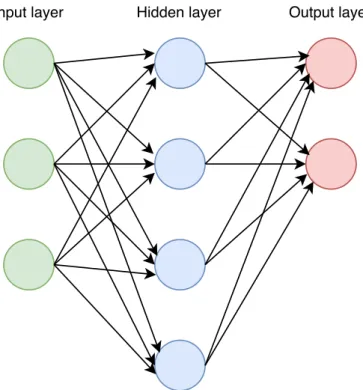
1.1.1 Structure

Each neural network consists of at least three layers: one input layer, one or more hidden layers, and one output layer. An example of a traditional neural network with three layers is shown in Figure 1.1. The following paragraph looks at the three types of layers (input, hidden, and output) in more detail. The purpose of the input layer is to distribute all components of an input vector into all nodes of the first hidden layer. The number of nodes in the in-put layer equals to the length of the inin-put vector. The hidden layers together with the output layer build the core of neural networks. Through the learn-ing process (also called the trainlearn-ing process), described later in Section 1.1.3,

(22)

1. Artificial Neural Networks

Figure 1.1: Structure of a simple 3-layer neural network.

they learn to solve a certain problem.2 The number of hidden layers, as well as the number of nodes in these layers, are one of the several hyperparamet-ers which have to be set and which usually depend on a particular problem. With increasing number of hidden nodes, artificial neural networks can tackle more complex data, but they are more difficult to train and more prone to overfitting. In this case, a neural network appropriately learns the data it is trained on but cannot generalise for previously unseen data, called the testing set. The output layer, connected to the last hidden layer, produces an output vector for each input vector. The number of nodes in the output layer equals to the length of the output vector.

1.1.2 Neurone

The nodes in the hidden layers and the output layer are artificial neurones. A scheme of such a neurone3 is depicted in Figure 1.2. The green nodes

x0, x1, . . . , xn are neurone’s inputs. For neurones in the first hidden layer,

the inputs represent an input vector. For neurones in other hidden layers or in the output layer, the inputs represent outputs of neurones in the previous

2

There are attempts to solve more problems at once by using only one neural network. For further information see for example article Progressive Neural Networks [9].

3

(23)

1.1. Feedforward Neural Networks

Figure 1.2: Artificial neurone.

layer. Each input xi has its weight wi. The weights and bias b (called also

threshold; bias = −threshold) are parameters of the neural network. These parameters are learnt during the learning process, described in the following section. The weighted inputs are summed, the bias is added and the result is put into the activation function f(Pn

i=0wi ·xi+b), represented by the blue

node. The common choice for the activation function is the sigmoid function

S(x) or the hyperbolic tangent tanh(x), which transform the input space into intervals (0,1) or (−1,1), respectively: S(x) = 1 1 +e−x tanh(x) = e 2x₋₁ e2x_{+ 1} 1.1.3 Learning

The weights and biases, discussed in the previous section, must be appropriate-ly adjusted to train the neural network. Let{(x1,y1),(x2,y2), . . . ,(xm,ym)}

be a training set where x_i is an input vector and y_i is an output vector. Let

g be a given function such that

(24)

for all i ∈ h1, mi. The learning problem consists of optimising the network weights and biases in a way that the network function λ approximates the function g. That is, the learning problem consists of minimising the error function4, defined as E = 1 2 m X i=1 ||o_i−y_i||2_, _(1.2)

whereoiare the output vectors of the network, i.e. λ(xi) =oifor alli∈ h1, mi.

When introducing new unknown input vectors to the network, it is expected to interpolate and to produce output vectors approximating outputs of the functiong.

Backpropagation, used as the learning algorithm to minimise the error function, is an iterative process repeating four steps:

1. forward propagation,

2. calculating the error function, 3. backward propagation,

4. updating the weights5.

There are three types of the backpropagation algorithm, depending on the number of input vectors used in one iteration. The on-line gradient descent uses only one randomly selected input vector. The off-line (also called full batch) gradient descent uses all inputs from the training set. And the mini-batch gradient descent uses a randomly selected subset of the training data.

The following paragraphs first outline the iteration process of the on-line gradient descent and later generalise it for the off-line and mini-batch gradi-ent descgradi-ents. During the first phase of the backpropagation algorithm, an input vector is propagated from the input layer through all hidden layers to the output layer. In the second phase, the error function (1.2) is calculated. Subsequently, the error is propagated backwards through the network to ana-lytically obtain the gradient of the error function with respect to all weights

∇E= _∂E ∂w1 , ∂E ∂w2 , . . . , ∂E ∂wr . (1.3)

4_{Called also the loss function, cost function or objective function. This particular error}

function is the mean squared error.

5

To simplify the notation used in this section, the biases are represented by extra weights connected to a node with output value 1.

(25)

1.1. Feedforward Neural Networks

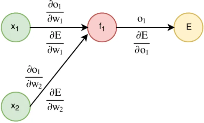
Figure 1.3: A simple network with two input nodes, one output neurone, and a node representing the error functionE.

The simple network in Figure 1.3 illustrates the calculating of the partial derivatives.6 This network has two inputs x1, x2, and one output neuronef1.

The node E represents the error function. During the forward propagation, the following is calculated for each neurone in all hidden and output layers of a neural network:

1. the output of the neurone,

2. partial derivatives of the output with respect to weights of all inputs connected to the neurone.

For the neurone f1 in Figure 1.3 the result (pictured above the edges) is

1. output o1,

2. ∂o1

∂w1

for the inputx1, and

∂o1

∂w2

for the input x2.

The error function E and the partial derivative of the error function with respect to the output of the output neurone ∂E

∂o1

is calculated in the second phase. During the backward propagation (pictured below the edges in Fig-ure 1.3), the partial derivatives of the error function with respect to the neur-one’s weights are computed using the chain rule:

6

(26)

1. Artificial Neural Networks 1. ∂E ∂w1 = ∂E ∂o1 · ∂o1 ∂w1 , 2. ∂E ∂w2 = ∂E ∂o1 · ∂o1 ∂w2 .

In the case of a network with more layers, the chain rule is applied iter-atively until the partial derivatives of neurones in all layers are calculated, resulting in the gradient in Formula (1.3).

The partial gradients can be as well calculated numerically, using the limit definition of a derivative ∂E ∂wi = lim h→0 E(wi+h)−E(wi−h) 2h ,

whereE(wi+h) is the error function for the same network in which only one

weight wi is changed. This numerical gradient is calculated for a few weights

and the result is compared to the analytical gradient. If there is no substantial difference, the gradient is used for updating the weights using the increment

∆wi =−γ

∂E

∂wi

for all i∈ h1, ri, (1.4) where γ is the learning rate influencing the speed of the learning process. A small learning rate means small increments, and usually slower learning. On the other hand, a large learning rate makes the network improve faster, but there is a higher probability of overlooking the optimum. A too large7learning rate can result in divergence instead of convergence of the error function.

The learning process of the on-line gradient descent, described above, is applicable to the off-line and mini-batch gradient descents after changes to the weights increments which look as follows,

∆wi= ∆1wi+ ∆2wi+· · ·+ ∆swi.

∆_jwi is the increment calculated for the input vector xj. The number of

increments s equals the size of the training set m for the off-line gradient descent, i.e. every input vector is used. For the mini-batch gradient descent, the number of increments 1< s < m represents the size of the batch.

The backpropagation algorithm is repeated as long as the error (the train-ing loss) decreases. These repetitions are counted in epochs. Durtrain-ing one epoch, every input vector is fed into the neural network once. The number of epochs largely influences the performance of the network as well as the

7

(27)

1.2. Convolutional Neural Networks

duration of the learning process. Therefore, it is important to interrupt the training of the network when the training loss has stopped decreasing. A com-mon solution is to implement the early stopping algorithm. This algorithm interrupts the learning process if the training loss has not improved for a spe-cified number of epochs. To prevent overfitting, the training data are split into a training set and a validation set. The backpropagation algorithm uses only the training set to adjust the network weights. At the end of each epoch, the validation loss is calculated using the validation set. The early stopping algorithm then compares the validation loss instead of the training loss.

The previous three sections described the structure of feedforward neural networks, their building blocks—artificial neurones, and the backpropagation algorithm used for training the networks. Various extensions and improve-ments of this architecture have been developed, such as convolutional neural networks, outlined in the following sections.

1.2 Convolutional Neural Networks

A common machine learning problem using neural networks can be separated into two parts. First, a hand-designed feature extractor selects the most rel-evant and important features from the data set. Second, a feedforward neural network is employed for a machine learning task using these features. Convo-lutional neural networks, described in this section, have a specifically designed architecture enabling an automatic extraction of the features.8

1.2.1 Structure

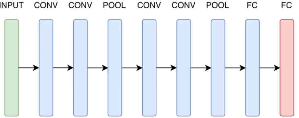
The structure of convolutional neural networks consists of three main build-ing blocks. Convolutional layers (CONV), poolbuild-ing layers (POOL), and fully-connected layers (FC). The composition of these layers commonly follows this pattern

IN P U T →[CON V ∗B →P OOL?]∗C →F C∗D→F C,

where IN P U T is the input layer, the last F C is the output layer, and the rest of the layers are the hidden layers. Symbol “∗” indicates repetition, symbol “?” indicates an optional addition of a layer preceding this symbol, and symbol “→” represents edges between layers. B, C, D≥0 are adjustable hyperparameters. Figure 1.4 shows a scheme of a convolutional network, where

B = 2, C = 2, and D = 1. The input layer is pictured in green colour, the 8

Moreover, convolutional neural networks give better results for inputs with a local structure (such as time series or images). [10] Object recognition in images is probably the machine learning field where the success of convolutional neural networks is best known. For further information, see, for instance, the article ImageNet Classification with Deep Convolutional Neural Networks [11].

(28)

hidden layers are blue (four convolutional layers, two pooling layers and one fully-connected layer), and the output layer is depicted in red colour. The following passages identify and explain in detail the three types of the hidden layers.

Figure 1.4: Scheme of a convolutional neural network withB = 2, C = 2, and

D= 1.

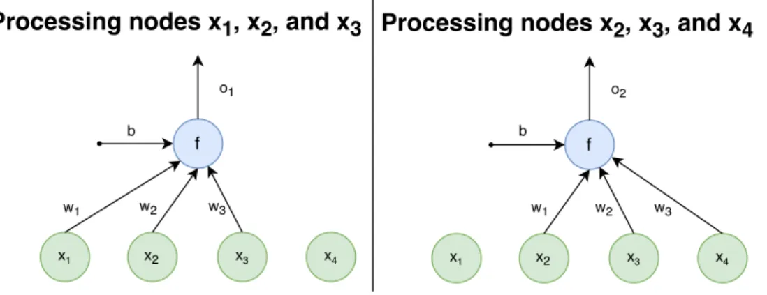
Convolutional Layer

A convolutional layer consists of several filters (also called local receptive fields) which can extract elementary features from an input vector. The num-ber of these filters is a hyperparameter of the network. Each filter is a neurone, as described in Section 1.1.2, connected to regions of the input vector. One such filter (labeledf) is depicted in Figure 1.5. The input vector (green nodes) of size four is divided into two overlapping regions. The first region (on the left side of the Figure 1.5) contains input nodesx1, x2, and x3 and produces

the outputo1. Input nodesx2, x3, andx4, producing the outputo2, belong to

the second region (on the right side of the Figure 1.5). For both regions, the filter’s weightsw1, w2, and w3 and bias bstay the same.

There are three hyperparameters specific for the convolutional layer: the filter size, the stride, and zero-padding. The filter size defines the size of the regions. The number of different nodes between two consecutive regions is determined by the stride. Lastly, zero-padding specifies the number of zero nodes (nodes with value zero) added to the edges of the input vector. Without these zero nodes, the edges of the input vector are processed fewer times than the rest of the input. In Figure 1.5, f ilter size = 3, stride = 1, zero

-padding= 0.

Pooling Layer

Outputs of the filters form so-called feature maps. A pooling layer, usually placed after a convolutional layer, reduces the dimension of the feature maps

(29)

1.3. Recurrent Neural Networks

Figure 1.5: The processing of two regions by one filter of size three, with zero-padding equal to zero and stride equal to one.

to make the network less prone to overfitting and to reduce the computational complexity. Pooling depends on two hyperparameters: the size of the pooling windows, and the stride, which is the downsampling factor. Two types of pooling are commonly used: average pooling and max pooling. The average pooling computes the average of its inputs and applies a non-linear function to this average. An output of the max pooling is the maximum of its in-puts. Scherer et al. [12] empirically show that the max pooling significantly outperforms the average pooling.

Fully-connected Layer

The extracted and down-sampled features are forwarded into one or more fully-connected layers. Neurones in such a layer are connected to all outputs of the neurones in the previous layer, as in the feedforward neural networks. By using these fully-connected layers, the neural network assigns an output vector to every input vector (such as a class in a classification task).

1.3 Recurrent Neural Networks

Feedforward neural networks make an assumption that all inputs are inde-pendent of each other. This is not an invalid assumption for most of the data sets, but seemingly not for all of them. Time series classification is an example of a machine learning problem using sequential inputs which are dependent on each other. Recurrent neural networks, also called neural networks with memory, however, are suitable for such problems due to their specific struc-ture. The following part analyses the structure and the learning algorithm: backpropagation through time.

(30)

Figure 1.6: Recurrent neural network unfolded into three time-steps with a sequential output.

1.3.1 Structure

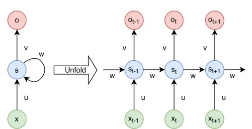
The structure of a recurrent neural network stays the same as described in Section 1.1.1. The only difference is that the network is evaluated more times in a row for all sequential components of an input (such as time points in a time series). Figure 1.6 demonstrates this process using a simple network with only one hidden neurone and a one-dimensional output. The left part of the Figure 1.6 shows the structure of the recurrent neural network. The node x is an input, the node s is the hidden state, and the node o is the network’s output. The information about the hidden state s is forwarded in a loop back to the hidden state. Similarly to feedforward neural networks, weights u, v and w, and bias b are parameters adjusted during the learning process. An advantage of recurrent neural networks is that all weights remain the same for the full sequential input. This significantly reduces the number of parameters as opposed to feedforward networks where weights change with every input.

The right part of the Figure 1.6 shows three time-steps of evaluating the network. In the time-stept, the hidden state stis calculated using the input

xt and the previous hidden state st−1 as

st=f(u·xt+w·st−1+b),

where f is the activation function discussed in Section 1.1.2. The output of the hidden statest is forwarded into the input of the next hidden statest+1.

This enables the network to process previous information.

Figure 1.6 depicts a network where both input and output are sequential. Examples of usage include text generating [13] and machine translation [14,

(31)

1.3. Recurrent Neural Networks

Figure 1.7: Recurrent neural network unfolded into three time-steps with a non-sequential output.

15]. However, there are machine learning problems where a non-sequential output is needed, such as time series classification. This introduces a small change into evaluating recurrent neural networks, pictured in Figure 1.7. The hidden state s(in the left part of the Figure 1.7) produces the output oonly for the last input (time-point) x. This process is depicted in the right part of the Figure 1.7, where hidden statesst−1, and st do not produce any outputs;

the only output ot+1 is given by the hidden state st+1.

1.3.2 Learning

This section introduces the learning algorithm of recurrent neural networks, called backpropagation through time. This algorithm is very similar to back-propagation described in Section 1.1.3. The error function is defined as

E =

l

X

t=0

Et, (1.5)

where lis the length of the output sequence and

Et=

1

2||ot−yt||

2_.

(y1, y2, . . . , yl) is the true output and (o1, o2, . . . , ol) is the output produced

by the network. For simplification, the error function of the on-line gradient descent is used, which contains only one output vector. The aim is to calcu-late the gradient of the error function with respect to all weights (such as in Equation (1.3)), where

(32)

Partial derivatives are then calculated as

∂E ∂wi = l X t=0 ∂Et ∂wi .

Considering a part of the unfolded network from Figure 1.6 for time-steps

{0,1, . . . , t}, the expression ∂Et

∂wi

is calculated as in the standard backpropaga-tion for feedforward networks.

1.3.3 Vanishing Gradient Problem

Backpropagation through time, discussed above, has a limitation called the vanishing gradient problem. Figure 1.8 pictures the sigmoid function and its derivative. It can be seen that the limits of the derivative approach zero at both ends. Multiplication of such small derivatives in the chain rule causes gradients at later time-steps to vanish.9 This implies an inability of recurrent neural networks to learn long-term dependencies in sequential inputs. One solution to this problem is using rectified linear units (ReLUs) [11], defined asf(x) = max(0, x), instead of the sigmoid or hyperbolic tangent activation functions. Another approach is offered by LSTMs, further described in the following section. 10.0 7.5 5.0 2.5 0.0 2.5 5.0 7.5 10.0 x 0.0 0.2 0.4 0.6 0.8 1.0 S(x), S'(x) S(x) S'(x)

Figure 1.8: The sigmoid function and its derivative.

1.4 Long Short-Term Memory Neural Networks

LSTMs were originally introduced by Hochreiter and Schmidhuber [17], and further improved by Gers, Schmidhuber, and Cummins [18]. Recurrent neural

9

(33)

1.4. Long Short-Term Memory Neural Networks

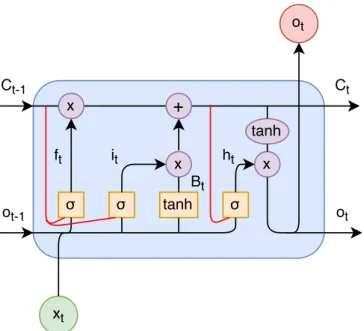
Figure 1.9: LSTM’s hidden unit.

networks with LSTMs share the same structure as well as the learning al-gorithm (backpropagation through time); the difference is in the hidden units, explained in the following passage.

1.4.1 Hidden Unit

A hidden unit of LSTMs is depicted in Figure 1.9. It consists of four parts: a cell state Ct, a forget gate ft, an input gate it and an output gate ht. The

cell state (represented by a number in this case and by a vector of numbers in the case of an input vector with more dimensions) functions as a memory of the unit containing all important information available in the sequential input vector. This information is selected and filtered by the three gates, described in detail in the following paragraphs. Each of the gates has its set of weights and biases. Weights uf and wf and bias bf belong to the forget

gate, weightsui, wi, ub, andwband biasesbiandbb are used by the input gate,

and the output gate contains weightsuhandwhand biasbh. Compared to the

recurrent neural networks, the higher amount of weights and biases increases the computational complexity of the learning process of LSTMs. However, it enables the LSTMs to learn long-term dependencies in the data.

The forget gate is responsible for deleting previously saved information from the unit’s cell state and is defined as

ft=σ(uf ·xt+wf ·ot−1+bf).

This gate uses the input xt and the output ot−1 of the previous hidden unit

(on the left of the Figure 1.9). The sigma function outputs a number between zero and one. If the output is zero, the information in the cell state will be fully deleted. In the case of an output equal to one, the information will be kept in the cell state.

(34)

Subsequently, the input gate, defined below, stores new information to the cell state:

it=σ(ui·xt+wi·ot−1+bi),

Bt= tanh(ub·xt+wb·ot−1+bb).

The sigma function in the input gate it selects what parts of the cell state

will be updated (in the case of a vector), and the hyperbolic tangent in Bt

specifies what values will be saved to these selected parts. The cell state is then updated as follows, using the forget gateftand the multiplication of the

input gateit and Bt:

Ct=it·Bt+ft·Ct−1.

The last part of the hidden unit is the output gateht, defined below, which

selects what parts of the cell state will be forwarded to the next hidden unit (the arrowot between the second and third blue node in Figure 1.9)

ht=σ(uh·xt+wh·ot−1+bh).

After this selection, the output gate ht is multiplied with the cell state to

obtain the actual information forwarded to the next hidden unit

ot=σ(ht·tanh(Ct)).

In the case of a sequential output, the same information is used as the output of the unit (the red nodeot in Figure 1.9).

Similarly to recurrent neural networks, all weights and biases are shared for the full sequential input and learnt during the learning process. After they are properly adjusted, the LSTM can learn the information contained in the input vector and use this information for producing an appropriate output (i.e. an output which minimises the error function (1.5)).

1.4.2 Peephole Connections

Gers and Schmidhuber [19] suggested a modification of this architecture by adding so-called peephole connections. Figure 1.10 pictures these connections (red lines). This enables all three gates to use the information contained in the cell state and to improve the performance of the network. The definitions of the gates change as follows:

ft=σ(uf ·xt+wf ·ot−1+pf ·Ct+bf),

it=σ(ui·xt+wi·ot−1+pi·Ct+bi),

ht=σ(uh·xt+wh·ot−1+ph·Ct+bh),

wherepf, pi andph are weights assigned to the peephole connections.

Accord-ing to [20], this architecture together with usAccord-ing full gradient trainAccord-ing [21] is the most commonly used architecture in literature.

(35)

1.4. Long Short-Term Memory Neural Networks

(36)

(37)

Chapter

2

Implementation

The principles and four different architectures of artificial neural networks were theoretically introduced in the previous chapter. Three of the architec-tures (convolutional, recurrent and long short-term memory neural networks) were implemented in order to compare them in the last part of this thesis. This chapter focuses on the implementation and is divided into two sections. Section 2.1 describes technical details of the implementation, including ar-chitecture, programming language, and libraries. Section 2.2 introduces the implemented program and specifies various settings of algorithms.

2.1 Technical Details

The implementation part of the thesis is written in Python [22], a high-level programming language widely used in machine learning. Its main advantage is a large variety of existing libraries, further described in the next section. The code was written and executed in The Jupyter Notebook [23], a conveni-ent web-based environmconveni-ent supporting many programming languages such as Scala, Ruby, R, JavaScript, and Python. The Jupyter Notebook was running in Docker [24], a software container, using the keras-full image [25].

As mentioned above, Python includes many useful libraries. The following list shortly describes six of them that were used in the implementation:

• Keras [26] is a high-level neural networks library running on top of either Theano or TensorFlow. Modularity and minimalism make it a very efficient tool for creating and experimenting with neural networks.

• TensorFlow [27] is an open source library for machine learning developed by Google. It features implicit scalability running on both CPUs and GPUs.

(38)

2. Implementation

• SciPy [28] is a library for scientific computing. Among others, it imple-ments a broad range of scientific functions.

• Numpy [29] is a Python extension introducing mainly N-dimensional array objects. It also includes an extensive library of mathematical functions to operate on these objects.

• Matplotlib [30] is a 2D plotting library. It offers various types of graphs such as plots, histograms, bar charts, and scatterplots.

• scikit-learn [31] is a machine learning library built on Numpy, SciPy, and Matplotlib. It implements many supervised and unsupervised al-gorithms, preprocessing methods, and model selection techniques.

2.2 Implementation Details

The previous section focused on the technical detailes of the implementation; this part describes various features of the experiment process and specific set-tings of the algorithms. The program offers three ways of optimising network hyperparameters: a manual search, a grid search, and a random search. The input of the manual search is a neural network model with defined hyperpara-meters. This model is trained on a training set and evaluated on a testing set. The program iteratively plots the training loss and the validation loss after every epoch. This process is repeated three times and the results are averaged in order to lower the effects of randomness.

The grid search and the random search automatically optimise all hyper-parameters using a cross-validation on a training set. The grid search takes sets of values of various hyperparameters as inputs. These sets are further de-scribed in Chapter 3. Inputs of the random search are uniform distributions of the hyperparameters values. The output of both functions is the selected best model and its hyperparameters. This model is then evaluated on a testing set using the manual search.

The following list describes specific settings of the algorithms:

• Early stopping is implemented for all methods, i.e. if the validation loss has not improved fornepochs, the training process stops. n= 5 during the grid search and the random search and n= 10 during the training process on the full training data set using the manual search. The min-imum change of the loss counting as an improvement is delta= 0.001. The maximum number of epochs is limited to 400.

(39)

2.2. Implementation Details

• The activation functionf used in the convolutional layers and the fully-connected layers (discussed in Section 1.2) as well as in the hidden layers of recurrent neural networks (described in Section 1.3) is the ReLU.

• The pooling layer is always added to the architecture of the convolutional neural networks.

• Zero-padding iteratively adds zeros to the front and the back of an input vector as long as the formula

(l−s+pf+pb) mod t

is not equal to zero. l represents the length of an input vector, pf and pb is the amount of zeros padded to the front and to the back of the vector, respectively. sstands for the size of the filter, and t is the filter stride.

• Output layers use the softmax function as the activation function defined as follows:

σ(z)j =

ezj

PK

k=1ezk

forj = 1, . . . , K, where z is a vector produced by the last hidden layer.

The lengthKof the vector represents the number of classes. The outputs of the softmax function for all components of the vector add up to one and can be interpreted as a categorical distribution.

• Categorical cross entropy is implemented as the loss function, using this categorical distribution.

(40)

(41)

Chapter

3

Experiments

The second chapter outlined the detailes of the implemented program. This program is used in the third chapter, which focuses on an experimental com-parison of two state-of-the-art architectures of neural networks and one baseline architecture: convolutional neural network, long short-term memory neural network, and recurrent neural network, respectively. The goal is to compare them in terms of their ability to learn, the effectivity of the training process and the classification performance. The first section describes these criteria and proposes an experimental design for their comparison. The experimental design includes three benchmark data sets, introduced in the second section. The last section compares the three network architectures on these data sets.

3.1 Experimental Design

This section is divided into two subsections. The first subsection focuses on experiments for comparing different architectures of neural networks. It lists and describes evaluation criteria and metrics, and proposes an experimental procedure. An important step in this procedure is to properly set neural network hyperparameters, in order to successfully train it on a given data set. A design of experiments used for finding the best hyperparameters for any given data set is presented in the second subsection.

3.1.1 Process of the Experiment

The first subsection focused on the process of the experiment contains three parts: evaluation criteria, evaluation metrics, and the experimental procedure.

Evaluation Criteria

Different architectures of neural networks are compared in terms of three criteria:

(42)

3. Experiments

• Theability to learn examines the structure of the networks, and how

changes in the structure influence the classification performance.

• Theeffectivity of the training processfocuses on the technical

para-meter, i.e. the time spent on training the network.

• Theclassification performancebelongs to one of the most important

metrics in a classification task. It measures how well the network ap-proximates the functiong (1.1), that is whether the network can learn the patterns in the data.

Evaluation Metrics

Each criterion has a different set of evaluation metrics, outlined in the fol-lowing list. These metrics are obtained during the experimental procedure, described in the last part of this subsection. Subsequently, the metrics are compared separately for each of the benchmark data sets.

Table 3.1: Structures of convolutional neural networks, defined using hyper-parametersB, C, and D. Number of layers B C D 3 1 1 1 4 2 1 1 5 1 2 1 6 1 2 2 7 2 2 1 8 2 2 2

• The ability to learn is analysed by plotting the dependency of the

classification performance on the number of neurones and the number of hidden layers. For LSTMs and recurrent neural networks, the lat-ter number means the number of layers containing LSTM and recurrent neurones, respectively. The performance is calculated for one to five hid-den layers. Table 3.1 shows structures of convolutional neural networks, defined using hyperparametersB, C, andD, as described in Section 1.2. The structures have six different depths (three to eight hidden layers). Set N = {5x|1 ≤ x ≤50} defines possible numbers of neurones for all architectures, as well as numbers of filters for convolutional networks.

• The effectivity of the training process is compared by measuring

the time of the training process.

• Theclassification performance is evaluated by comparing precision,

(43)

3.1. Experimental Design

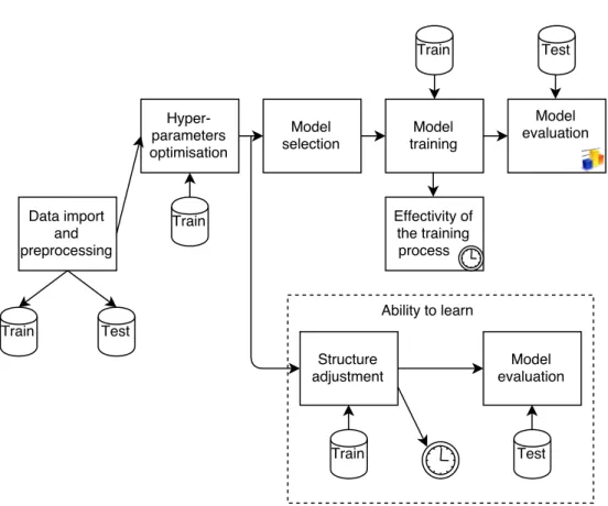
Figure 3.1: A graphical schema of the experimental procedure.

measures are compared separately for each class to determine whether there is a difference in the classification performance for various classes.

Experimental Procedure

The graphical schema in Figure 3.1 shows the experimental procedure. The data, divided into training and testing sets, are imported and transformed into a proper format. Both sets are randomly shuffled.10 The hyperparameters of all network architectures are optimised using the training set. This process is further described later in the following section. The model with the best classification performance is selected for each of the architectures.

The evaluation metrics are calculated by applying this model to the full data set. Stratified 70% of the training set is used in the learning process, and 30% is held out as the validation set for early stopping. The effectivity of the training process is measured. The model is subsequently applied to

10

The pseudorandom number generator seed is fixed for a better reproducibility of the results.

(44)

3. Experiments

the testing set, and the classification performance is evaluated. This process is repeated three times, and the evaluation metrics are averaged accordingly. The training set is always shuffled between iterations.

The classification performance in dependency on the structure is calcu-lated. The number of neurones and the number of layers are selected from the sets described in the second part of this subsection. Other hyperparamet-ers are fixed according to the selected model. An exhaustive grid search is executed, resulting in 5·50 = 250 models for recurrent neural networks and 6·50 = 300 models for convolutional networks. These models are trained on the training data and tested on the testing data. This process is repeated three times, and the results are averaged.

3.1.2 Hyperparameters

Hyperparameters are variables defining neural network’s higher-level proper-ties such as its structure. They are set before the training process, i.e. before optimising the network parameters.

Recurrent Neural Networks

The following list shortly describes hyperparameters of recurrent neural net-works.

• Thelearning rate influences the speed of the learning process by

con-trolling how much the weights change during each update. For more information see Equation (1.4).

• Thelearning rate decaysets the speed at which the learning rate

de-cays. A high learning rate has the advantage of a fast learning process and a broad exploration of the space of the loss function values. On the other hand, a small learning rate decreases the loss steadily and enables exploring parts of the search space which would be unreachable with a high learning rate. The learning rate decay combines the advantages of both. It sets a high learning rate at the beginning of the learning pro-cess and continually decreases it by little steps. However, Bengio [32] recommends keeping the learning rate constant. To reduce the complex-ity of the experimental design, this recommendation is followed.

• The optimiser is another important hyperparameter. Sections 1.1.3

and 1.3.2 describe the stochastic gradient descent (SGD) as the back-propagation algorithm, but more optimisers have been developed, such as RMSprop, Adagrad, Adadelta, Adam, Adamax, and Nadam.

(45)

• The number of epochs, further described in Section 1.1.3, influences

the performance of the network and the length of the training process. Early stopping interrupts the training process if the validation loss has not improved for a defined number of epochs. Therefore, this hyper-parameter is not optimised.

• The size of the batch is another hyperparameter. As described in

Section 1.1.3, the mini-batch gradient descent (and other optimisers) use only a subset of the training set for updating the weights. A small batch means more updates and a broader exploration of the weights space. A bigger batch enables more precise gradient descent, however only locally, because the descent keeps changing during iterations.

• The number of hidden layers specifies the depth of the network.

Deeper networks are usually able to better generalise from the data because of their ability to learn features at more levels of abstraction. On the other hand, larger networks are more prone to overfitting.

• The number of neurones in each hidden layer defines the width of

the network and together with the number of layers forms its structure. Bengio [32] states that a larger number of neurones usually works better because the network can generalise well and the negative effects of over-fitting are reduced by regularisation (see Dropout below).11 Bengio also argues that using the same amount of neurones in each layer generally works better or the same as using a decreasing or increasing size.

• Weights initialisation is an important step at the beginning of the

learning algorithm. These eight initialisers are tested: uniform, lecun uniform, normal, zero, glorot normal, glorot uniform, he normal, and he uniform.

• Dropout [33] is a regularisation technique used to avoid overfitting.

During training, randomly selected units along with their connections are dropped out from the network. This makes the network less sensitive to specific settings of weights, thus prevents it from co-adapting too much to the training data. The tunable hyperparameter is the dropout rate, i.e. the amount of dropped out neurones.

• Batch normalisation[34] can be placed after each layer that includes

activation functions. As the network parameters change during training, the distribution of the activations changes as well. This phenomenon is called internal covariate shift and it slows down the training process. Batch normalisation reduces the shift by normalising network activations during every batch update. The hyperparameter controls whether it is added into the network’s architecture.

11

(46)

3. Experiments

These hyperparameters are not independent of each other and cannot be adjusted separately. Instead, the grid search is used, which is capable of optimising more hyperparameters simultaneously. However, they cannot be optimised all at once because of the exponential computational complexity of the grid search. Therefore, they are divided into five smaller subsets:

1. {number of neurones, number of layers, dropout rate}, 2. {optimisers, learning rate},

3. {learning rate, batch normalisation, dropout rate}, 4. {weights initialisation},

5. {batch size, learning rate}.

The values of the hyperparameters are limited as well:

• learning rate ∈ {0.00001, 0.0001, 0.001, 0.01, 0.1},

• optimisers ∈ {SGD, RMSprop, Adagrad, Adadelta, Adam, Adamax,

Nadam},

• batch size∈ {1, 2, 3, 4, 8, 16, 32},

• number of layers∈ {1, 2, 3, 4, 5},

• number of neurones∈ {50, 100, 150, 200, 250},

• weights initialisation∈ {uniform, lecun uniform, normal, zero, glorot

normal, glorot uniform, he normal, he uniform},

• dropout rate∈ {0.0, 0.2, 0.4, 0.6, 0.8},

• batch normalisation ∈ {true, false}.

The experimental procedure for choosing the hyperparameters given a data set has five iterations. During each iteration, the grid search returns the best values for a subset of the hyperparameters, which are fixed before the next iteration. Evaluation of the values of the hyperparameters is based on cross-validation, where the training set is split into four stratified folds. Three models are learnt using two of these folds as training data, one fold as a val-idation set used by the early stopping algorithm, and the remaining fold as a testing set.

(47)

The random search is another optimisation technique showing good res-ults as well [32]. During each iteration, every hyperparameter is randomly selected from the uniform distribution of its values. Thus, the random search can effectively search in the hyperparameter space. This technique is tested alongside the grid search, and the better model is selected.

Convolutional Neural Networks

The experimental procedure, introduced above, can be used for both recurrent neural networks and convolutional neural networks, but the set of hyperpara-meters differs. The number of layers is extended to three hyperparahyperpara-meters,

B,CandD, as described in Section 1.2. That section also introduces six more hyperparameters specific for convolutional networks: thenumber of filters, thesizeof each filter, thestride, thezero-padding, thepooling size, and

the pooling stride. To reduce the time complexity of the optimisation

al-gorithm, the pooling size and the pooling stride are fixed to the value 2. The ordered list of subsets of the remaining hyperparameters looks as follows:

1. {number of neurones, number of filters, B, C, D}, 2. {number of neurones,D, dropout rate},

3. {filter size, filter stride}, 4. {optimisers, learning rate},

5. {learning rate, batch normalisation, dropout rate}, 6. {weights initialisation},

7. {batch size, learning rate}.

The values are limited to these subsets:

• learning rate ∈ {0.00001, 0.0001, 0.001, 0.01, 0.1},

• optimisers ∈ {SGD, RMSprop, Adagrad, Adadelta, Adam, Adamax,

Nadam},

• batch size ∈ {1, 2, 3, 4, 8, 16, 32},

• number of neurones∈ {50, 100, 150, 250},

• number of filters ∈ {50, 100, 150, 250},

(48)

3. Experiments

• filter stride ∈ {1, 2, 3},

• B ∈ {1, 2},

• C ∈ {1, 2},

• D∈ {1, 2},

• weights initialisation∈ {uniform, lecun uniform, normal, zero, glorot

normal, glorot uniform, he normal, he uniform},

• dropout rate∈ {0.0, 0.2, 0.4, 0.6, 0.8},

• batch normalisation ∈ {true, false}.

Three filter sizes are defined as ratios of the length n of a time series, as recommended by [35].

3.2 Benchmark Data Sets

The architectures are compared on three time series classification data sets. This section theoretically introduces time series and classification and de-scribes single data sets.

3.2.1 Time Series

A time series is a set of sequentially collected observations. In the case of equally spaced time points, it is a set {yt}, where t∈Z is the time at which

an observation was taken. If the observations are not equally spaced in time, the notation is {yti}, where i ∈ N. Time series are usually represented by

plots. Two examples are in Figures 3.2 and 3.3.

A multivariate time series is a set of time series with the same timestamps. Following the notation from above, for equally spaced time points, it is a set

{{y1t},{y2t}, . . . ,{yqt}}, whereq is the number of univariate time series (also

called features), and t∈ _Zis the time. In the case of unequally spaced time points, it is a set{{y1ti},{y2ti}, . . . ,{yqti}}, wherei∈N.

3.2.2 Classification

Supervised learning is a machine learning task, where training examples are pairs consisting of an input and a corresponding output. Classification is a subset of supervised learning, where outputs represent classes (categories). The classification problem consists of sorting inputs into correct classes. More formally, a training set has a form of{(x1, y1),(x2, y2), . . . ,(xm, ym)}, where

x_iare input vectors, andyiare corresponding classes. Time series classification

(49)

3.2. Benchmark Data Sets 0 20 40 60 80 100 120 140 t 1.0 0.5 0.0 0.5 1.0 yt

Figure 3.2: An example of theGun-Draw class from the Gun-Point data set.

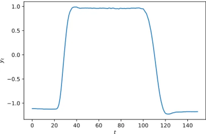
0 20 40 60 80 100 120 140 t 1.0 0.5 0.0 0.5 1.0 yt

Figure 3.3: An example of thePoint class from the Gun-Point data set.

3.2.3 Data Sets

Time series classification data sets used in the experimental part of this thesis come from the UCR Time Series Classification Archive [36], and the UCI Machine Learning Repository [37].

Gun-Point

The first set is the Gun-Point data set, originally published by Ratanama-hatana and Keogh [38]. It contains 200 univariate time series, 50 of them belong to the training set and 150 to the testing set. The time series were obtained by tracking the motion of the right hand of one male and one female actor. The data set is divided into two classes: Gun-Draw and Point.

(50)

3. Experiments 0 50 100 150 200 t 1 0 1 2 3 yt

Figure 3.4: An example of theStrawberry class from the Strawberry data set.

Both classes begin with the actors standing and having both hands at their sides. In the Gun-Draw class, they reach for a gun stored in a holster, which is mounted at their hips. They draw the gun at an imaginary opponent for approximately one second, return it to the holster and put their hands back to their sides. In thePoint class, they only point their index fingers at the opponent and put their hands back to their sides. The time series are composed of the x-coordinates of the centroids of their hands tracked during these procedures. Examples of time series for theGun-DrawandPoint classes are shown in Figures 3.2 and 3.3, respectively. It can be seen that there are two lumps in the first figure, as the actor had to reach for the gun. No such lumps are in the Point class figure.

Strawberry

The Strawberry data set, published in [39], comes from the field of food ana-lysis. It contains 983 univariate time series, divided into the training (370) and testing (613) set. Two classes were obtained using Fourier transform infrared spectroscopy of strawberry pur´ees for a Strawberry class and non-strawberry (such as raspberry, apple, blackberry or adultered non-strawberry) pur´ees for a Non-Strawberry class. An example of the Strawberry class is in Figure 3.4.

Japanese Vowels

The Japanese Vowels data set, originally collected by Kudo et al. [40], is a part of the UCI Machine Learning Repository [37]. It is split into the training set (270 time series) and the testing set (370 time series). All time series are multivariate and contain 12 features. Each time series represents a sound of

(51)

3.3. Comparison of Architectures 0.0 2.5 5.0 7.5 10.0 12.5 15.0 17.5 20.0 t 1.5 1.0 0.5 0.0 0.5 1.0 1.5 2.0 yt

Figure 3.5: The Japanese Vowels data set.

two Japanese vowels /ae/ uttered successively by one of nine male speakers, forming a set of nine classes. The features are 12 LPC cepstrum coefficients obtained from the 12-degree linear prediction analysis. An example of the time series is in Figure 3.5.

3.3 Comparison of Architectures

The three data sets, introduced above, are used for the comparison of three ar-chitectures of neural networks. Every set is compared in a separate subsection. Each architecture is represented by one best model with a set of hyperpara-meters found during the optimisation process. These models are compared in terms of the ability to learn, the effectivity of the training process, and the classification performance.

3.3.1 Gun-Point

The first subsection focuses on the smallest of the data sets, the Gun-Point data set. The following paragraphs list the optimised hyperparameters and compare the ability to learn, the effectivity of the training process, and the classification performance.

(52)

3. Experiments

Table 3.2: Optimised hyperparameters for the Gun-Point data set.

RNN LSTM CNN

Learning rate 0.0001 0.000684 0.003244

Optimiser Adamax Adamax RMSprop

Batch size 1 27 17

Number of layers 3 4

Number of neurones 100 100 182

Weights initialisation glorot normal he uniform glorot uniform

Dropout rate 0.0 0.439786 0.24793

Batch normalisation False False False

Number of filters 128 Filter size 3 Filter stride 2 B 1 C 1 D 2 Hyperparameters

Table 3.2 shows the optimised hyperparameters for three architectures: recur-rent neural network (RNN), long short-term memory neural network (LSTM), and convolutional neural network (CNN). The random search found better models than the grid search for two architectures (LSTM and CNN). For the RNN, the model selected by the grid search had better classification perform-ance than the model selected by the random search.

Ability to Learn

Figure 3.6 shows the classification performance (F-score) in dependency on the number of neurones (x-axis) and the number of layers (different colour shades) for CNNs. All results were calculated for up to 250 neurones, but because of no further information in the data, the plots are limited to 150 neurones. Networks with seven or eight layers are generally worse on this data set than networks with fewer layers. The classification performance seems to be correlated with the number of neurones for smaller architectures (five to approximately 30 neurones). For architectures with more than 30 neurones, the performance fluctuates but does not change on average. The classification performance for the CNN architecture on the Gun-Point data set cannot be concluded independent on the structure of the network.

The classification performance in dependency on the number of neurones and the number of layers for LSTMs can be seen in Figure 3.7. The classific-ation performance increases with the number of neurones for networks with