Department of Economics
University of St. Gallen
Robust Value at Risk Prediction
Loriano Mancini, Fabio Trojani
Editor: Prof. Jörg Baumberger University of St. Gallen Department of Economics Bodanstr. 1 CH-9000 St. Gallen Phone +41 71 224 22 41 Fax +41 71 224 28 85 Email [email protected] Publisher: Electronic Publication: Department of Economics University of St. Gallen Bodanstrasse 8 CH-9000 St. Gallen Phone +41 71 224 23 25 Fax +41 71 224 22 98 http://www.vwa.unisg.ch
* Correspondence Information: Loriano Mancini, Swiss Banking Institute, University of Zurich, Plattenstrasse 14, 8032 Zurich, Switzerland, phone: +41(0)44 634 2942, fax: +41(0)44 634 4997, E-mail: [email protected]. E-mail address for Fabio Trojani: [email protected]. We gratefully acknowledge the financial support of the Swiss National Science Foundation (NCCR-FinRisk and Grants Nr. 101312-103781/1 and 100012-105745/1) and the University Research Priority Program “Finance and Financial Markets” University of Zurich. We thank Claudio Ortelli and Claudia Ravanelli for many valuable suggestions on an earlier draft. Much of this paper was written while Mancini visited the Department of Operations Research and Financial Engineering, Princeton University, whose hospitality is gratefully
Robust Value at Risk Prediction*
Loriano Mancini, Fabio Trojani
Author’s address: Prof. Dr. Fabio Trojani
Institut für Banken und Finanzen Rosenbergstrasse 52 9000 St. Gallen Tel. +41 71 2247074 Fax +41 71 2247088 Email [email protected] Website www.sbf.unisg.ch
Abstract
We propose a general robust semiparametric bootstrap method to estimate conditional predictive distributions of GARCH-type models. Our approach is based on a robust estimator for the parameters in GARCH-type models and a robustified resampling method for standardized GARCH residuals, which controls the bootstrap instability due to influential observations in the tails of standardized GARCH residuals. Monte Carlo simulation
showsthat our method consistently provides lower VaR forecast errors, often to a large extent, and in contrast to classical methods never fails validation tests at usual significance levels. We test extensively our approach in the context of real data applications to VaR prediction for market risk, and find that only our robust procedure passes all validation tests at usualconfidence levels. Moreover, the smaller tail estimation risk of robust VaR forecasts implies VaR prediction intervals that can be nearly 20% narrower and 50% less volatile over time. This is a further desirable property of our method, which allows to adapt risky
positions to VaR limits more smoothly and thus more efficiently.
Keywords
Backtesting, M-estimator, Extreme Value Theory, Breakdown Point. JEL Classification
1
Introduction
Large portfolios of traded assets held by many financial institutions have made the measurement of market risk, i.e. the risk of losses on the trading book due to adverse market movements, a primary concern for regulators and internal risk managers. The Basel Committee (1996) requires that financial institutions hold a certain amount of capital against market risk. This capital is called Value at Risk (VaR) and must be sufficient to cover losses on the trading book over a ten days holding period 99% of the times. In practice, VaR measures are computed for several holding periods and confidence levels. For internal purposes, for instance, most banks use VaR at a 95% confidence level and a horizon of one day. From a statistical viewpoint, VaR is the quantile of the profit and loss (P&L) distribution of a portfolio over a certain holding period. Hence, a key issue in implementing VaR and related risk measures is to obtain accurate estimates for the tails of the conditional P&L distribution at the relevant horizons. In the financial literature two main direc-tions have been followed to estimate P&L conditional distribudirec-tions for market risk management: fully nonparametric historical simulation methods and semiparametric/nonparametric bootstrap methods based on dynamic models for asset returns; see Duffie and Pan (1997) for an overview. Fully nonparametric methods are easy to implement, but unfortunately do not provide accurate VaR predictions. Semiparametric methods have been found to work well and are commonly called Filtered Historical Simulation (FHS) methods; see, among others, Pritsker (1997), Hull and White (1998), Diebold, Schuermann, and Stroughair (1998), Barone-Adesi, Giannopoulos, and Vosper (1999), McNeil and Frey (2000), Pritsker (2001), and Kuester, Mittnik, and Paolella (2006). In these papers, parametric GARCH-type models for returns are fitted using pseudo maximum likelihood (PML). Then standardized GARCH residuals are resampled using either (i) a fully non-parametric bootstrap or (ii) a seminon-parametric bootstrap based on PML estimations of generalized Pareto distributions for the tails of GARCH residuals. Therefore, semiparametric methods allow for time varying conditional moments of returns (via parametric GARCH-type models) and
non-parametric structures in conditional distribution of returns (as GARCH residual distributions are estimated nonparametrically). The last feature is crucial in applications and avoids too simplistic assumptions on return conditional distributions, such as normality; see for instance JP Morgan’s RiskMetrics (1995). In contrast to a fully nonparametric method, the semiparametric approach resamples approximately iid standardized GARCH residuals without relying on resampling pro-cedures for non iid data and the necessary assumptions for those to hold; see for instance K¨unsch (1989).1
In this paper we propose a class of robust semiparametric bootstrap methods to estimate con-ditional predictive distributions of asset returns in GARCH-type volatility models. This approach can account for general parametric specifications of time varying conditional mean and variance of asset returns. As an application, we use the proposed robust method to compute Value at Risk predictions over different forecasting horizons. Our robust approach combines a robust esti-mator for parametric GARCH-type volatility dynamics and a robustified resampling method for standardized GARCH residuals. Hence, robustness is achieved in two steps. In the first step, we estimate a parametric GARCH-type model using the optimal bounded influence estimator in Mancini, Ronchetti, and Trojani (2005). In the second step, we fit the robust generalized Pareto density estimator in Dupuis (1999) and Ju´arez and Schucany (2004) to the tails of the GARCH residuals distribution and we resample from this distribution. In order to ensure robustness of the whole bootstrap procedure, both robustification steps are necessary. It is well-known that outliers
1A potentially alternative way to estimate risk measures for P&L distributions is to apply directly statistical tools
designed to estimate regression quantiles and conditional distributions; see for instance Koenker and Bassett (1978), Foresi and Peracchi (1995), Peracchi (2002), and Engle and Manganelli (2004). From a robustness perspective, drawbacks of regression quantiles are their behavior under heteroscedasticity and the non robustness to “bad” leverage points; see Koenker and Bassett (1982). Moreover, regression quantile methods are naturally applied to one day ahead VaR predictions, as illustrated in Engle and Manganelli (2004). Their efficient extension to the estimation of risk measures for longer horizons is, however, not straightforward.
or influential points in the data can strongly bias and highly inflate PML parameter estimates of GARCH-type models; see for instance Sakata and White (1998) and Mancini et al. (2005). In our semiparametric bootstrap context, this feature can induce inaccurately estimated GARCH residuals and unreliable bootstrap distributions. In addition, standard bootstrap procedures suf-fer from an intrinsic robustness problem, especially when bootstrapping fat tailed distributions. A small number of outliers in the data can cause the breakdown of quantile estimates based on nonparametric bootstrap distributions of residuals; see for instance Singh (1998), Davidson and Flachaire (2005), Gagliardini, Trojani, and Urga (2005) and Camponovo, Scaillet, and Trojani (2006). The robust extreme value estimator in our approach controls the bootstrap instability deriving from outliers or influential points in the tails of GARCH residual distributions. We show that the standard nonparametric bootstrap procedure has a low breakdown point, meaning that VaR forecasts can be heavily affected by a few influential points, especially when long forecast horizons are considered. Robustness can be enhanced by fitting a generalized Pareto distribution to the tails of the residual distribution and sampling tail residuals from this density. Sampling from a parametric density can circumvent the robustness problem of nonparametric bootstrap procedures. However, to ensure a sufficiently large breakdown point for the estimator of the gen-eralized Pareto tails, a robust extreme value estimator is needed. Such an estimator is not subject to the instability problem of PML estimators for generalized Pareto distributions as noted, among others, in Cowell and Victoria-Feser (1996).
Extreme or outlying observations—due for instance to abnormal liquidity conditions or market crashes—are a fundamental component of data generating processes of financial returns and, in particular, of the riskiness we aim to measure. Therefore, they cannot be simply disregarded when estimating measures of market risk. However, such observations are typically caused by relatively rare market conditions that are very difficult to anticipate using historical return information and almost impossible to model conveniently in a simple parametric model for asset returns, such
as a GARCH-type model. To avoid biased GARCH estimates that are not representative for the typical volatility dynamics in the data, we estimate a parametric GARCH model with the bounded influence estimator proposed in Mancini et al. (2005). To ensure the stability of the GARCH residual bootstrap procedure we fit the robust generalized Pareto estimator in Dupuis (1999) and Ju´arez and Schucany (2004) to the tails of the GARCH residual distribution.
We study the accuracy of VaR predictions at 5% and 1% confidence levels for one day and ten days ahead forecast horizons by performing Monte Carlo simulation and in real data applications. Monte Carlo simulation shows that compared to the non robust counterparts our robust proce-dure suffers very moderate efficiency losses, when estimating a GARCH model with conditionally Gaussian innovations. At the same time, it offers substantial improvements in accuracy under sev-eral forms of departure from conditional normality, which are likely to be present in financial data. Procedures based on classical methods imply less reliable VaR predictions under conditionally non Gaussian data, especially for several days ahead horizons. In particular, in the presence of outlying observations, robust VaR predictions at 1% confidence level have mean square prediction errors several times smaller than those of classical procedures. In nearly all Monte Carlo experiments and for all VaR confidence levels and forecast horizons, our robust bootstrap procedure has the lowest mean square prediction errors, often by a large extent. Moreover, in contrast to classical methods our procedure never fails validation tests based on VaR violations at 10% level.
The simulation evidence is confirmed by the real data application. We backtest VaR predic-tion methods using about twenty years of S&P 500, Dollar-Yen, Microsoft and Boeing historical returns. Overall, robust VaR predictions are found to be more accurate than classical ones: in our backtesting exercises the robust VaR forecasting method is the only one that passes all valida-tion tests at a 10% significance level, both for all VaR confidence levels and all forecast horizons. Moreover, the robust procedure implies a smaller tail estimation risk, which is reflected by robust VaR prediction intervals that are more accurate and more stable over time. For instance, in the
case of S&P 500 and Boeing, robust VaR prediction intervals are nearly 20% narrower and 50% less volatile than classical ones. In risk management, the stability over time of VaR predictions is a desirable feature, because financial institutions cannot adjust rapidly the capital base. At the same time, stable VaR profiles over time allow to adapt outstanding portfolio risk exposures to VaR limits more smoothly and thus more efficiently. Therefore, the time stability of VaR predic-tions estimated by robust semiparametric bootstrap methods is a further desirable property of our approach.
Section 2 introduces semiparametric bootstrap and extreme value estimation methods for VaR predictions, along with their robust versions. Section 3 presents Monte Carlo simulation com-paring the performance of classical and robust, nonparametric and semiparametric, bootstrap VaR prediction methods, under different forms of conditional non normality of returns. Section 4 presents the real data application to VaR prediction and backtesting for four financial time series. Section 5 concludes.
2
Setting
This section introduces the different semiparametric bootstrap procedures for GARCH-type mod-els relevant for our analysis.
2.1
Return Dynamics and Measures of Market Risk
Let Y := (Yt)t∈Z be a strictly stationary time series process on probability space (R∞,F,P∗),
modelling the daily rate of return on a financial asset with pricePtat timet, i.e.Yt:=Pt/Pt−1−1.
We assume that P∗ can be “approximated” by some parametric model P := {Pθ, θ ∈ Θ ⊆ Rp}.
Precisely, P∗ ∈ U(Pθ
distribution G. Under Pθ
0, process Y satisfies the dynamic model
Yt=µt(θ0) +σt(θ0)Zt, (1)
where µt(θ0) and σt2(θ0) parameterize the conditional mean and conditional variance of Yt, given
information Ft−1 up to time t−1. Under probability Pθ0, innovations Zt’s are a strong white
noise, i.e.Zt ∼IIN(0,1). We denote by F the distribution function ofZtunderP∗. Given Y1m :=
(Y1, . . . , Ym), denote by Pm∗ (Pmθ0) the m-dimensional marginal distribution of Y
m
1 under P∗ (Pθ0).
Ft,t+h is the conditional distribution function of h days returns Yt,t+h := Pt+h/Pt−1 under P∗, given informationFt. For 0< α <1 and horizonhdays, lower quantileyt,tα+hofFt,t+his defined by
yt,tα+h := inf{y ∈R:Ft,t+h(y)≥α}.
The Value at Risk (VaR) at time t of an institution investing in a portfolio of assets with market
price Pt is V aRαt,t+h =Pt+Rαt,t+h, where Rαt,t+h is the reserve amount such that the probability of
a loss over the next h days is not above some levelα:2
α=P∗(Pt+h+Rα
t,t+h <0|Ft) =P∗(Pt+h−Pt<−V aRαt,t+h|Ft). (2)
In other words, −V aRα
t,t+h = Ptyt,tα+h is the α-quantile of the conditional profit and loss (P&L)
distribution underP∗over the nexthdays, givenFt. In contrast to historical simulation techniques,
V aRα
t,t+h reflects current available information such as high or low volatility periods, which is
important to achieve accurate VaR forecasts.3 Another measure of market risk is the Expected
Shortfall (ES) Sα
t,t+h (Artzner, Delbaen, Eber, and Heath (1999)), defined by
St,tα+h :=E∗[Yt,t+h|Yt,t+h < yαt,t+h, Ft],
where E∗[·] denotes expectation with respect toP∗.4 For horizon h= 1 day,
yαt,t+1 =µt+1(θ0) +σt+1(θ0)zα , St,tα+1 =µt+1(θ0) +σt+1(θ0)E∗[Z|Z < zα],
2To simplify the exposition, equation (2) is based on a continuous profit and loss distribution underP
∗.
3See for instance Gouri´eroux, Laurent, and Scaillet (2000) for a general discussion on conditional VaR, and
A¨ıt-Sahalia and Lo (2000) for an economic interpretation of VaR in a general equilibrium model.
where zα is the α-quantile of the distribution of Zt. Hence estimation of VaR or ES can be
obtained by (i) estimating model (1) for daily conditional moment dynamics and (ii) estimating the tail distribution of daily standardized residual Zt. For longer horizons h ≥ 2, estimated
daily dynamics are only the starting point to estimate Ft,t+h. Joint conditional distributions
of (Zt+1, . . . , Zt+h), (µt+1, . . . , µt+h) and (σt+1, . . . , σt+h) have to be estimated, a task which is
considerably more difficult. Filtering Historical Simulation (FHS) methods estimate Ft,t+h by
applying a semiparametric bootstrap to dynamic model (1) over horizon [t, t+h].
Our goal is to develop robust semiparametric bootstrap methods for estimatingFt,t+h. In this
setup, underlying distribution P∗ is unknown and belongs to some nonparametric neighborhood
of parametric reference model Pθ
0. HencePθ0 has to be regarded as an “approximate” description
of the true data generating process P∗.
2.2
Estimations of GARCH-type Dynamics
We use pseudo maximum likelihood (PML, Gouri´eroux, Monfort, and Trognon (1984)) estimators for the parameters of dynamic model (1) and bounded influence, conditionally unbiased, optimal versions of such PML estimators (Mancini, Ronchetti, and Trojani (2005)).
2.2.1 Pseudo Maximum Likelihood Estimation
Typically, model (1) is estimated by a PML approach, under the nominal assumption of Gaussian innovations. The functional PML estimator (PMLE) a(·) is implicitly defined by the asymptotic estimating equation E∗[s(Y1m;a(Pm∗ ))] = 0, where s(Y1m;θ) = 1 σ2 m(θ) ∂µm(θ) ∂θ εm(θ) + 1 2σ2 m(θ) ∂σ2 m(θ) ∂θ ε2 m(θ) σ2 m(θ) − 1 (3)
and εm(θ) :=σm(θ)Zm. Under model Pθ0, PMLE and MLE coincide, implying an asymptotically
optimal covariance matrix
V(s;θ0) = Eθ0[s(Y
m
1 ;θ0)s(Y1m;θ0)⊤]−1 =:I(θ0)−1,
where I(θ0) is the information matrix. However, if Pθ0 is slightly different from the true data
generating process forY, PML estimators can induce highly biased and inefficient inference results on θ0; see for instance Sakata and White (1998) and Mancini et al. (2005). In Section 3, we
investigate by Monte Carlo simulation how such estimates affect Value at Risk forecasts under several realistic forms of local departures from conditional normality in model (1).
2.2.2 Optimal Robust Estimation
As a robust estimator for conditional moment dynamics in model (1) we use the optimal condi-tionally unbiased bounded-influence estimator for GARCH-type models developed in Mancini et al. (2005). Such a robust estimator is efficient and computationally feasible for highly nonlinear models, and compares therefore favorably with other robust estimators, such as robust GMM es-timators (Ronchetti and Trojani (2001)) or robust EMM eses-timators (Ortelli and Trojani (2005)) for time series. It is defined as follows. Let
ψc(s(Y1m;θ)) :=A(θ) s(Y1m;θ)−τ(Ym −1 1 ;θ) w(Y1m;θ), where s(Ym
1 ;θ) is the PML score function defined in (3) and the weighting function
w(Y1m;θ) := min(1, ckA(θ) s(Y1m;θ)−τ(Ym−1
1 ;θ)
k−1).
Define a robust functional M-estimator a(·) of θ implicitly by
where non singular matrix A(θ)∈Rp×Rp and Fm−1-measurable random vector τ(Ym−1
1 ;θ)∈Rp
are determined by the implicit equations
Eθ0[ψc(s(Y m 1 ;θ0))ψc(s(Y1m;θ0))⊤] = I, (5) Eθ0[ψc(s(Y m 1 ;θ0))|Fm−1] = 0. (6)
The estimating function ψc is a truncated version of PML score (3) and can be interpreted as a
weighted PML score because by constructionkψc(s(Y1m;θ))k ≤c. Constant c≥√pis selected by
the researcher and controls the degree of robustness of the estimatora. It can be chosen according
to an estimator’s efficiency criterion (as in Mancini et al. (2005)) or based on a more inference oriented principle (see Ronchetti and Trojani (2001)). As in this paper we are interested in efficient estimates of GARCH-type models (the preliminary step in our robust semiparametric bootstrap method), we apply an efficiency criterion in Section 2.4 to select c. Note that when c= ∞, a is the PMLE of θ0 underP∗.
Formally, optimality results in Mancini et al. (2005) hold for Markovian estimating functions, which encompass ARCH-type, but not GARCH-type processes. As in Sakata and White (1998), however, we can realistically expect that our robust estimator performs satisfactorily also under well-behaved GARCH models with sufficient memory decay. Moreover, we can use a Markovian estimating function implied by an approximating ARCH-type process with a sufficient number of lags in the corresponding conditional variance function. For instance, in the standard GARCH(1,1) model we can rewrite the conditional variance σ2
t(θ0) as an invertible ARMA process,
σt2(θ0) = α0+α1ε2t−1(θ0) +α2σ2t−1(θ0) = +∞ X j=0 αj2 α0+α1ε2t−1−j(θ0) = l−1 X j=0 αj2 α0+α1ε2t−1−j(θ0) +αl2σt2−l(θ0) =:σt2(θ0)trunc+αl2σt2−l(θ0) ≈ σ2t(θ0)trunc,
and use the approximation in the last row, as for a sufficiently large laglwe can expectαl
0. Of course, the bounded-influence estimator atrunc based on σ2t(θ0)trunc is slightly biased, but
such a bias can be expected to be negligible for a sufficiently largel. In our Monte Carlo simulation
(Section 3), we compare robust procedures based on both non Markovian GARCH-type estimating functions and Markovian ARCH-type estimating functions based on a truncated GARCH volatility function. We find that for the lag l= 30 estimation results under these two methods are virtually
identical. These results are discussed in Section 3.1.
To implement a semiparametric bootstrap for VaR estimation, conditional mean and condi-tional volatility dynamics of model (1) have to be specified. A substantial amount of empirical evidence suggests that financial asset return volatility is stochastic and mean reverting, return innovations are non-normal, and equity return volatility responds asymmetrically to positive and negative returns; see for instance Ghysels, Harvey, and Renault (1996). In discrete time settings, the stochastic volatility is often described using GARCH model introduced by Engle (1982) and Bollerslev (1986). Comprehensive surveys of the GARCH and related models are Bollerslev, Chou, and Kroner (1992) and Bollerslev, Engle, and Nelson (1994). Several different GARCH-type mod-els for asset returns have been proposed in the financial literature. Our robust bootstrap method can accommodate quite general parametric specifications for conditional mean and conditional variance of asset returns. The different specifications imply different estimating functions, but do not change the overall procedure. In our simulations and empirical applications, we adopt a fairly flexible semiparametric model for asset returns. We assume an AR(1) model for the conditional mean µt(θ0) and an asymmetric GARCH(1,1) model for the conditional variance σt(θ0) (Glosten,
Jagannathan, and Runkle (1993)),
µt(θ0) = ρ0+ρ1Yt−1, (7)
σt2(θ0) = α0+α1ε2t−1(θ0) +α2σt2−1(θ0) +α3ε2t−1(θ0)It−1(θ0), (8)
where α0, α1, α2 > 0, |ρ1| < 1, α1 + α2 + α3/2 < 1, It−1(θ0) = 1 when εt−1(θ0) < 0, and
returns, for instance due to nonsynchronous transactions in different index components. α3 > 0
accounts for the leverage effect,5 that is the stronger impact of “bad news” (ε
t−1(θ0) < 0) than
good “good news” (εt−1(θ0)≥0) on conditional varianceσt2(θ0). Compared to symmetric GARCH
models, asymmetric GARCH models are better able to fit volatility dynamics of equity and index returns; see for instance Engle and Ng (1993) and Engle and Rosenberg (2002). To our knowledge, however, robust estimators of asymmetric GARCH processes have not yet been applied in the statistics and econometrics literature.
2.3
Robust Semiparametric Bootstrap of GARCH-type Processes
We study semiparametric bootstrap methods for GARCH-type processes consisting of two steps: 1. A preliminary estimation of the AR(1), asymmetric GARCH(1,1) model (7)–(8).
2. A bootstrap procedure for estimated scaled residuals in model (7)–(8).
In the first step, we use the PML and the optimal robust estimators in Section 2.2. Given observed daily rate of returns y1, . . . , yT, we denote by ˆθ = (ˆρ0 ρˆ1 αˆ0 αˆ1 αˆ2 αˆ3)⊤ the estimated parameter
vector in model (7)–(8), obtained either by PML or optimal robust estimator. In the second step, we apply bootstrap estimators of FT,T+h, based on different bootstrap procedures for estimated
scaled residuals in model (7)–(8). Estimated scaled residuals from the asymmetric GARCH(1,1) model are defined by
ˆ
zt=
yt−µt(ˆθ)
σt(ˆθ)
, t= 1, . . . , T,
5The name leverage effect was introduced by Black (1976) who suggested that a large negative return increases
the financial and operating leverage, and rises equity return volatility; see also Christie (1982). Campbell and Hentschel (1992) suggested an alternative explanation based on the market risk premium and volatility feedback effects; see also the more recent discussion by Bekaert and Wu (2000). We shall use the name leverage effect as it is commonly used by researchers when referring to the asymmetric reaction of volatility to positive and negative return innovations.
where conditional means and conditional volatilities {µt(ˆθ), σt(ˆθ)}Tt=1 are computed recursively
from (7)–(8) after having substituted sensible starting values. We denote by PT the empirical
distribution of estimated scaled residuals ˆz1, . . . ,zˆT. Engle and Gonzalez-Rivera (1991) introduce
and investigate the theoretical properties of semiparametric GARCH models driven by empirical innovations ˆzt. Applying the robust estimator (4) extends the estimation of such GARCH models
to the robust setting.
Accurate parameter estimates ˆθ are of critical importance as they determine the dynamics of
conditional means and conditional volatilities as well as the estimated scaled residuals ˆzt. Optimal
robust estimatora(·) can provide accurate parameter estimates of model (7)–(8) under conditional non normality of general form and in the presence of outliers or other influential points. In contrast, classical PML estimates can be highly biased and inefficient in such a setting. Monte Carlo simulation (Section 3) investigates these issues.
2.3.1 Nonparametric Residual Bootstrap and VaR Estimation
Nonparametric residual bootstrap relies on the nonparametric empirical estimator PT as an
esti-mator of the innovation distribution F. Estimation of one day ahead VaR forecast ˆyα
T,T+1 for
horizon h = 1 day is easily obtained by means of the empirical quantile ˆzα of PT, yielding
ˆ
yα
T,T+1 =µT+1(ˆθ) +σT+1(ˆθ) ˆzα.
Estimation of VaR measures for horizonsh≥2 days is more involved and obtained as follows. Select randomly with replacement scaled innovations z⋆
1, . . . , zh⋆ from PT. Compute recursively
bootstrap daily returns y⋆
T+1, . . . , yT⋆+h and portfolio prices p⋆T+1, . . . , p⋆T+h as follows.
• For y⋆
T+1 and p⋆T+1:
• For y⋆ T+j and p⋆T+j, j = 2, . . . , h: yT⋆+j = ˆρ0 + ˆρ1yT⋆+j−1+σT⋆+jzj⋆, p⋆T+j =p⋆T+j−1(1 +y⋆T+j), where σ⋆T+j = (ˆα0+ ˆα1σ⋆T2+j−1zT⋆2+j−1+ ˆα2σT⋆2+j−1+ ˆα3σT⋆2+j−1zT⋆2+j−1IT⋆+j−1)1/2, with I⋆ T+j−1 = 1 ifzT⋆+j−1 <0, andIT⋆+j−1 = 0 otherwise.
UsingB= 10,000, say, bootstrap samples{z1⋆(b), . . . , zh⋆(b)}B
b=1 compute an estimate ofFT,T+has the
bootstrap distributionF⋆
T,T+hofhdays ahead simulated returns yT,T⋆ +h :=p⋆T+h/pT−1. Thehdays
ahead VaR forecast at 1% level, say, is given by the 1% empirical quantile of distribution F⋆
T,T+h.
The bootstrap method provides an estimate of the entire conditional predictive distributionFT,T+h
and other risk measures, such as Expected Shortfall, can be readily computed.
2.3.2 Breakdown Analysis of Nonparametric Residual Bootstrap
Bootstrap estimateF⋆
T,T+his obtained by nonparametric bootstrap of estimated scaled innovations
ˆ
z1, . . . ,zˆT. Such innovations can well include a certain amount of outliers or influential points. Via
the resampling procedure, such observations can heavily affect the estimated quantiles of F⋆
T,T+h
and hence the corresponding VaR forecasts. To investigate this issue, we compute the bootstrap breakdown point of quantile estimates implied byF⋆
T,T+h; see also Singh (1998). Letbα denote the
breakdown point of VaR forecast ˆyα
T,T+h implied byFT,T⋆ +h. That is,T bα is the smallest number of
scaled innovations in the original sample that need to go to −∞ in order to force ˆyα
T,T+h to go to
−∞. In practice, scaled innovations do not go to −∞ and ˆyα
T,T+h could be unreliable well before
reaching−∞. The asymptotic definition of the breakdown point is a convenient tool to assess the robustness property of an estimator. By definition, T bα is an integer between 1 and T. Without
loss of generality, we assume the outliers causing the breakdown of ˆyα
T,T+h to be in the lower tail
Proposition 1
bα = 1−(1−α)1/h.
Proof. See Appendix A.
Hence the breakdown point bα →0 whenh→+∞. That is, for a longer horizonh fewer outliers
are sufficient to carry ˆyα
T,T+h to −∞. For h = 1 day, bα = α as the α-quantile is estimated by
the corresponding empirical quantile of PT. Table 5 presents numerical values of bα for different
horizons h. Given the very low breakdown point prevailing for longer horizons, such as ten days,
we can expect a quite bad performance of bootstrap estimates ˆyα
T,T+h implied by nonparametric
residual bootstrap, already under a moderate number of outliers or influential points in the data. Our Monte Carlo simulation in Section 3.4 confirms this conjecture.
2.3.3 Semiparametric Residual Bootstrap and VaR Estimation
Semiparametric residual bootstrap with Extreme Value Theory (EVT) relies on a different esti-mator of the innovation distribution F. Instead of using nonparametric estimator PT, the basic
idea is to approximate the lower and upper tail of F by means of a parametric generalized Pareto
distribution (GPD) whose distribution function Gξ,β is
Gξ,β(x) = 1−(1 +ξx/β)−1/ξ, ξ6= 0, 1−exp(−x/β), ξ= 0,
where the support of Gξ,β is [0,+∞) for ξ ≥ 0, and [0,−β/ξ] for ξ < 0. To estimate the upper
tail of F with a GPD, fix a “high” threshold u (such as the 90th percentile of {zˆj}Tj=1). Then for
any k > u
P∗(Zt> k) = P∗(Zt> u) P∗(Zt> k|Zt> u) =P∗(Zt> u) P∗(Zt−u > k−u|Zt> u). (9)
In (9), P∗(Zt > u) is easily estimated nonparametrically by estimator PT
j=11{zˆj > u}, where
threshold ucan be approximated with a generalized Pareto distribution using the limit result (see
Balkema and de Haan (1974) and Pickands (1975))
lim
u→x 0≤supx<x−u|F¯u(x)−Gξ,β(u)(x)|= 0,
where x is the (finite or infinite) right endpoint of F and β(u) is a positive measurable function.
To estimate lower tail of F with a GPD, fix a “low” thresholdu <0 (such as the 10th percentile
of {zˆj}Tj=1) and apply for every k < u the above procedure to excess lossesx =−(k−u) using a
GPD with distribution function Gξ,β(−u).
Given GPD parameter estimates ˆξ(1),βˆ(1) and ˆξ(2),βˆ(2) for the lower and the upper tail of F,
scaled innovations z⋆
1, . . . , zh⋆ are sampled from PT and adjusted as follows. For j = 1, . . . , h:
a) If z⋆
j < u, sample a GPD( ˆξ(1), ˆβ(1)) distributed excess loss x1 and returnu−x1.
b) If z⋆
j > u, sample a GPD( ˆξ(2), ˆβ(2)) distributed excess gain x2 and return u+x2.
c) If u≤z⋆
j ≤u, return scaled residualzj⋆ itself.
Using adjusted scaled residuals, semiparametric bootstrap methods apply the same procedure as in Section 2.3.1 for nonparametric residual bootstrap in order to estimate the conditional predictive density FT,T+h.
2.3.4 Pseudo Maximum Likelihood and Robust Estimations of Generalized Pareto
Distribution
Sampling scaled innovations from a parametric GPD tail can circumvent the robustness problem of standard nonparametric residual bootstrap procedures. However, GPD parametersζ := (ξ, β)⊤
have to be estimated and also it can be important to ensure the robustness of the GPD( ˆξ(1), ˆβ(1))
and GPD( ˆξ(2), ˆβ(2)) tails. In our Monte Carlo simulation and empirical application, we use the
Letq(·) denote the PML estimator for the GPD parameters and G∗ the true tail distribution
of threshold exceedances X,q(·) is defined by the asymptotic estimating equation
EG∗[sgpd(X;q(G∗))] = 0,
where sgpd(x;ζ) is the GPD score function
sgpd(x;ζ) = sξ(x;ζ) =ξ−2log(1 +ξx/β)−(1 + 1/ξ)(1 +ξx/β)−1x/β sβ(x;ζ) =−β−1+ (1 + 1/ξ)β−1(1 +ξx/β)−1ξx/β . (10)
As the score function sgpd(x;ζ) is unbounded in x, this estimator is not robust. Given positive
constantcgpd ≥
√
2, optimal bounded influence estimator of GPD parameters, notedq, is implicitly
defined by the estimating equation (see Dupuis (1999))
EG∗[ψc(sgpd(X;q(G∗)))] = 0, (11)
where sgpd(x;ζ) is the GPD score function (10) and
ψc(sgpd(X;ζ)) := A(ζ) (sgpd(X;ζ)−τ(ζ))w(X;ζ),
w(X;ζ) := min 1, cgpdkA(ζ) (sgpd(X;ζ)−τ(ζ))k−1
.
Matrix A(ζ) and vectorτ(ζ) are solutions of the equations
Eζ0 ψc(sgpd(X;ζ0))ψc(sgpd(X;ζ0))⊤ = I Eζ0[ψc(sgpd(X;ζ0))] = 0.
The GPD is the natural limiting distribution of a large class of tail distributions; see Embrechts, Kl¨uppelberg, and Mikosch (1997) for details. Hence it is reasonable to assume that the true tail distribution of the data, G∗, can be approximated by a GPD distribution Gζ
0, say. However,
several authors have emphasized the instability of PML estimator for GPD distribution when a moderate number of influential points is present in the sample; see for instance Cowell and Victoria-Feser (1996) and references therein. Optimal robust estimator q in (11) can provide
accurate GPD parameter estimates also in such problematic settings. Furthermore, as shown in Ju´arez and Schucany (2004), estimator q compares favorably also with respect to more involved
robust extreme value estimators when the true distribution has support [0,+∞), which is the relevant case for our application.
2.4
Choices of Threshold Levels and Robustness Tuning Constants
The choice of thresholds u and u in EVT applications determines the trade-off between bias and
variance of the estimator for GPD parameters. Based on Monte Carlo evidence, McNeil and Frey (2000) suggest to use the empirical 10th and 90th quantiles of {zj}Tj=1, i.e.u=z0.10 andu=z0.90,
for estimating lower and higher quantiles in risk management applications.6 In our Monte Carlo
experiments and empirical applications we select such thresholds for PML and robust estimators of GPD.
An important choice in the application of robust estimators for GARCH models and for GPD is the tuning constantscandcgpdin (4) and (11), respectively. Such constants control the degree of
robustness of estimators. Following Mancini et al. (2005), we set the levels of cand cgpd to achieve
a given asymptotic efficiency under the reference models Pθ
0 and Gζ0. To our knowledge, this
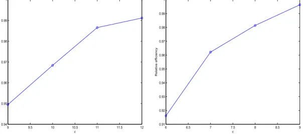
approach has not yet been applied in models with highly nonlinear dynamics as those studied here. Figure 5 illustrates the relative efficiency of estimators a and q with respect to the corresponding
ML estimators under the reference models Pθ
0 and Gζ0, as a function of constant c and cgpd.
For example the relative efficiency of a is measured as trace(V(s; ˆθn))/trace(V(ψc; ˆ¯θn)), where
asymptotic covariance matrices V are estimated using n = 20,000 observations simulated under
the reference model Pθ
0, s is the ML score function in (3), ˆθn the ML estimate, ψc the estimating
function of the robust estimator in (4) and ˆ¯θn the optimal robust estimate. In our Monte Carlo
6McNeil and Frey (2000) find that the resulting quantile estimates are rather insensitive to threshold levels for
simulation, the choicec= 11 for robust estimatoraimplies approximately 98% asymptotic relative
efficiency (see the left plot in Figure 5). The relative efficiency for q is computed analogously and
the choice cgpd = 8 implies an asymptotic relative efficiency of about 98% (see the right plot in
Figure 5).
3
Monte Carlo Simulation
We compare the performance of semiparametric bootstrap for GARCH processes based on (i) PML or robust estimators for GARCH-type models, introduced in Section 2.2, and (ii) nonparametric or semiparametric residual bootstrap methods, introduced in Section 2.3.
PML GARCH Robust GARCH
Empirical dist. fhs fhs rob
PML GPD evt —
Robust GPD — evt rob
For brevity, we call the VaR prediction method based on nonparametric residual bootstrap fhs; see the above panel. When GARCH dynamics are estimated with the robust estimator (4) we call this method fhs rob; evt rob uses robust estimators both for GARCH dynamics and for GPD tail estimations, while evt uses standard PML estimators at both stages. Comparing fhs and fhs rob VaR predictions allows to assess the potential improvement of VaR forecasts due to robust instead of PML estimation of the GARCH model. In Section 3.4 we compare VaR forecasts of previous methods based on the true GARCH parameters. In that context comparing evt and evt rob allows to assess the potential improvement of VaR forecasts due to robust instead of PML estimation of tail distributions. Hence the simulation design allows to evaluate the contribution of each robustification step to the accuracy of VaR predictions.7
7Considering the two hybrid cases PML GARCH/Robust GPD and Robust GARCH/PML GPD in the above
To study the accuracy of the different methods, we compute out-of-sample VaR forecasts at 1% and 5% confidence levels for horizonsh= 1 day andh= 10 days, under an AR(1), asymmetric
GARCH(1,1) model for daily returns. Precisely, we simulate the following dynamics for Y. 1. Student t5 innovation model. In this experiment, scaled innovation in model (1) is given by
Zt = ((ν−2)/ν)1/2Tν, (12)
where random variableTν has a Student-tdistribution withν = 5 degrees of freedom. Hence
Zt ∼IID(0,1) and model (1) is dynamically correctly specified.
2. Laplace innovation model. Scaled innovation in (1) is given by
Zt = 2−1/2L, (13)
where random variable L has a Laplace (or Double exponential) distribution. Such a
dis-tribution has a symmetric convex density and displays fatter tails than the t5 distribution.
Also in this experiment Zt∼IID(0,1) and model (1) is dynamically correctly specified.
3. Replace-innovative model. Under such a model observed process Y := (Yt)t∈Z is generated
according to the data generating process
Yt= ρ0+ρ1Yt−1+εt, with probability 1−κ, ˇ Yt, with probability κ, (14)
where ˇYt ∼ N(0, ̺2), εt ∼ N(0, σt2) and σt2 is given by (8). Hence at time t there is a
probability κ that observation Yt is not generated by the GARCH dynamics. The possible
“shock” ˇYt will affect future realizations of the process, mainly by “inflating” the conditional
variance on subsequent days. In this experiment, model (1) is “slightly” misspecified as the dynamic equations (7)–(8) are not satisfied for every t. We set κ = 0.2% and ̺ = 10.
The probability of contamination, κ, is very low and implies (on average) 4 contaminated
of the different VaR estimators under very infrequent, but dramatic, (symmetric) shocks. Such shocks could occur over short time periods in real data, as for instance in daily equity returns.
We simulate an AR(1), asymmetric GARCH(1,1) model for the following parameter choice ρ0 =
ρ1 = 0.01, α0 = 0.03, α1 = 0.02, α2 = 0.8, and α3 = 0.2, under the above distributions for Yt
and for a sample size T = 2,000. This parameter choice reflects somehow parameter estimates
typically obtained for daily percentage index or exchange rate returns; see for instance Bollerslev et al. (1994). At the reference model Pθ
0, annualized volatility of Yt is about 12%. The tuning
constants for the robust GARCH estimators a and atrunc are c = 11. The one for the robust
GPD estimator q is cgpd = 8. Each model is simulated 1,000 times. For each simulated sample
path, we estimate the model (7)–(8) using classical and robust estimators and we apply the four VaR prediction methods (fhs, fhs rob, evt, evt rob) to compute conditional VaR forecasts (as a percentage of pT) at confidence levels α = 5%, 1% and horizons h = 1 day, 10 days ahead.
In the financial industry, virtually only out-of-sample VaR forecasts are required and in-sample measurements of VaR are by far less important. In our simulations and empirical applications, all VaR forecasts are out-of-sample ones.
3.1
GARCH Dynamics Estimation
Table 1 presents bias and mean square error (MSE) (in percentage) of PML, robust and “trun-cated” robust parameter estimates, a and atrunc, for the AR(1), asymmetric GARCH(1,1) model
(7)–(8); see also Figures 1–4. Under reference model Pθ
0, PMLE (which is indeed MLE) is only
slightly more efficient than the robust estimators of GARCH models. In all other experiments, robust estimators always outperform classical PML estimator in terms of mean square errors. In particular, under the contaminated replace-innovative model, both robust estimators largely out-perform the PML estimator. Under all considered models, the overall out-performances of the two
robust estimators a and atrunc are very close, althougha has somewhat lower mean square errors.
We interpret the last finding in support of the application ofato dynamic models with estimating
functions depending on an infinite number of process coordinates, such as GARCH models.
3.2
VaR Violations
Table 2 shows the number of violations of fhs, fhs rob, evt and evt rob VaR forecasts for horizons
h = 1 day, 10 days, and confidence levels α = 5%, 1%. In the i-th simulation, a violation occurs
when the actual loss is larger than the predicted VaR, i.e.I(i) :=1{yT,T+h(i)<yˆT,Tα +h(i)}= 1 and
zero otherwise. Under the null hypothesis that the proposed method estimates the VaR correctly, the test statistic P1000
i=1 I(i) is binomially distributed, Bin(1000, α), as the 1,000 simulations are
independently drawn. Hence for α = 0.05 and 0.01 the expected number of violations are 50
and 10, and two-side confidence intervals at 95% level are [37,64] and [4,17], respectively. For all
horizons and VaR confidence levels, Table 2 shows that all methods exhibit numbers of violations within such intervals. Hence apparently all methods are rather accurate in forecasting VaR, when relying only on violation tests. Indeed, it is known that FHS-type VaR forecasts tend to display the proper number of violations; see for instance Kuester, Mittnik, and Paolella (2006) for a recent comparison of these methods. However, Table 2 also hints some differences among VaR prediction methods. In the first two Monte Carlo experiments (Student t5 and Laplace innovation models),
only evt rob never exhibits test p-values below 0.10, even though estimated GARCH models are
correctly specified. These results suggest that evt rob can outperform other approaches even in setups relatively favorable to classical methods, but this aspect is not clearly detected by violation tests. In the next section we study the precision of VaR forecasts, which, of course, plays a key role in measuring market risk.
In our simulation study VaR violations both at horizonsh= 1 day and 10 days are all mutually
to test for VaR violations accurately. In empirical applications, VaR violations are not necessarily independent and it is standard practice to apply the independence test proposed by Christoffersen (1998).8 In the empirical application (Section 4) we apply also the independence and other tests.
3.3
VaR Prediction
Left panel in Table 3 shows bias and MSE of fhs, fhs rob, evt and evt rob in predicting VaR at
h= 1 day ahead horizon and α= 5%, 1% confidence levels. The true VaR is computed under the
true data generating process. In all experiments the robust versions of FHS and EVT methods outperform the corresponding classical versions in terms of MSE. The reduction in VaR forecast MSE is small in the Laplace innovation model, but reaches about 80% in the contaminated replace-innovative model. In particular, fhs rob provides more accurate VaR forecasts than fhs because relies on more accurate estimates of volatility dynamics; see Table 1. In all but one case, evt rob has the lowest VaR forecast MSE.
Right panel in Table 3 shows the accuracy of VaR predictions at h = 10 days horizon. The
true VaR is obtained by simulating 100,000 times true dynamics for Y over the ten days horizon [T, T + h]. In the first two experiments the dynamic model (1) is correctly specified and all
VaR prediction methods tend to perform similarly in predicting VaR at 5% level, although evt rob outperforms all other methods in predicting VaR at 1% level. In the third experiment the dynamic model (1) is misspecified and both FHS methods perform very poorly, with fhs rob having the largest MSE for VaR prediction at the 1% level. At first sight, the last finding might appear puzzling given the higher accuracy of robust GARCH estimates documented in Table 1. The result is explained by the very low breakdown point of VaR predictions based on nonparametric residuals bootstrap and the larger absolute residuals produced by robust estimation in this case.9 This
8The independence test would be trivially verified in the present simulation setup.
9To raise the breakdown point of nonparametric bootstrap quantiles, Singh (1998) suggests to winsorize the
point is discussed in more detail in Section 3.4 below. In terms of MSE, robust EVT predictions largely outperforms all other methods, often by several orders of magnitude. These findings put in perspective the results based on violation tests discussed in the previous section. Even though the estimated GARCH model is misspecified and evt rob provides more accurate VaR predictions, violation tests have a quite low power in discriminate among the different VaR prediction methods; see Table 2. Measuring the precision of VaR forecasts reveals that evt rob largely outperforms all other methods. In our empirical application (Section 4), we report common violation test results and measure, in addition, the precision of VaR forecasts by investigating model estimation risk.
3.4
Residual Bootstrap Breakdown Point and Quantile Estimates
Accuracy
The accuracy of above bootstrap procedures for GARCH-type processes depends on the accu-racy of (i) GARCH parameter estimates and (ii) quantile estimates implied by GARCH residuals bootstrap. We showed above that robust GARCH parameter estimators have higher accuracy under different forms of conditional non normality of returns. To deepen the analysis of the rel-ative accuracy between residual nonparametric bootstrap and residual semiparametric bootstrap using EVT, we repeat the previous Monte Carlo simulation using true GARCH parameters in the estimation of scaled residuals ˆz1, . . . ,zˆT. In this way, we eliminate estimation errors due to
GARCH parameter estimation and we can disentangle the contribution of nonparametric, classical and robust EVT methods to VaR predictions. We also investigate the theoretical predictions of Proposition 1 on breakdown points of bootstrap quantiles.
We estimate 5% and 1% quantiles (VaR) of ten days ahead return distribution. As GARCH parameters are not estimated classical and robust FHS methods coincide and we call them simply
computed VaR predictions using classical and robust FHS over ten days horizon. MSE’s of the winsorized VaR predictions did decrease, but only by a small amount and the results are not reported.
“resampling” in this section. We also consider different ways of implementing semiparametric bootstrap methods using EVT. We make an additional distinction depending on whether the quantile of simulated ten days ahead distribution is estimated empirically or using a GPD (PML or robust) estimator. This distinction highlights the additional contribution of parametric GPD over nonparametric tail estimations in producing accurate VaR forecasts.10 Summarizing, we
compute VaR predictions using the following five approaches: 1. Resampling (FHS),
2. EVT applied to both daily returns and to simulated ten days ahead returns,
3. Robust EVT applied to both daily returns and to simulated ten days ahead returns,
4. EVT applied to daily returns, and empirical quantile estimation applied to ten days ahead returns,
5. Robust EVT applied to daily returns, and empirical quantile estimation applied to ten days ahead returns.
Table 4 presents simulation results for the five bootstrap methods under the previous three Monte Carlo experiments. As expected, all MSE’s of VaR forecasts in Table 4 are lower than the corre-sponding ones in Table 3, as variability deriving from estimation of GARCH parameters is absent now. In the first two experiments (Student t5 and Laplace innovations), the data generating
processes do not produce “outliers”. Resampling procedures and robust EVT perform satisfac-torily for quantiles at the 5% level. Classical EVT method is the least precise in this case, by a large amount for the Laplace innovations case. For 1% quantiles, robust EVT methods have a uniformly higher accuracy.
10In all previous simulations, classical and robust EVT estimations were always applied to both daily and ten
Under the replace-innovative model, nonparametric resampling method breaks down in the estimation of the 1% quantile in the presence of 0.20% outliers in the data, whereas it produces accurate results in estimating 5% quantiles. From Table 5, the breakdown point of VaR at 5% level corresponds to 0.51% contamination by outliers, whereas the breakdown point of VaR at 1% level is 0.10%. Hence as predicted by Proposition 1, 0.20% of outliers breaks down VaR predictions at 1%, but not VaR predictions at 5% obtained by nonparametric residual bootstrap.11 In predicting
VaR at 1%, robust EVT method applied both to daily and ten days ahead returns has the lowest MSE across all simulation experiments. Overall, applying robust EVT estimators to both daily and ten days ahead returns seems to be particulary important when forecasting VaR at low confidence level 1% and/or data are contaminated by outliers. Given the very small percentage of outliers generated in our simulations (0.20%) and the difficulties documented for the other methods, VaR forecasts based on robust EVT and robust GARCH estimations can be expected to be the most reliable ones in many realistic applications.
4
Real Data Estimation and Backtesting
We backtest VaR prediction methods on four historical series of daily rate of returns: the S&P 500 index from December 1988 to July 2003, the Dollar-Yen exchange rate from January 1986 to January 2005, Microsoft share price from March 1986 to January 2005, and Boeing share prices from January 1980 to January 2005. The data are downloaded from Datastream. To backtest the four VaR prediction methods on a historical series y1, . . . , yN, whereN ≫n, we compute the
out-of-sample VaR forecast ˆyα
T,T+h for each T ∈ T ={n, n+ 1, . . . , N −h} using a time window
of n historical daily returns for each estimation. We set n = 2,000 and hence about eight years
of data were used for each estimation. For each day T ∈ T, we predict VaR’s at horizons h = 1 day, 10 days, and confidence levels α = 1%, 5%, using fhs, fhs rob, evt and evt rob. AR(1),
asymmetric GARCH(1,1) model is estimated using the PML estimator (3) and the optimal robust estimator (4) with tuning constantc= 8, the estimates are updated every 500 days and the tuning
constant of the optimal robust GPD estimator is cgpd= 6.12
4.1
Data and GARCH Estimation
Table 6 shows summary statistics for the daily rate of returns. As expected, different assets have different characteristics. For example, Dollar-Yen exchange rates have relatively high skewness and Microsoft returns high kurtosis unconditionally. These different characteristics make the backtest-ing exercise particularly interestbacktest-ing. Table 7 shows the AR(1), asymmetric GARCH(1,1) model (7)–(8) estimates given by classical PML and robust a estimators. In several occasions and
espe-cially for the volatility parameters the two estimates are rather different and next sections show how they induce different VaR forecasts. Interestingly, the asymmetry parameter a3 turns out to
be (very close to) zero for the Dollar-Yen exchange rates. This parameter controls the asymmetric impact of positive and negative shocks on conditional variance. As negative shocks or depreci-ations of one currency correspond to positive shocks or apprecidepreci-ations of the other, asymmetric effects can be absent in exchange rates. For example, using options data Xu and Taylor (1994) document symmetric, instead of skewed, implied volatility smiles for exchange rates, confirming no asymmetric impact of shock returns on volatility.
4.2
Backtesting VaR Prediction
To assess the forecasting performance of the different VaR prediction methods we adopt the testing framework proposed by Christoffersen (1998). Although this framework has become a
12Considering the “noisier” nature of real data, as opposed to simulated data, and the different characteristics of
financial time series (indexes, stocks and exchange rates) used in backtesting, we take a somewhat more conservative viewpoint setting the robustness tuning constantsc andcgpd to lower levels than in the Monte Carlo study.
standard theoretical framework for evaluating out-of-sample forecasts, for completeness and to setup the notation we briefly recall it here as well; see also Christoffersen (2003). Denote by
It :=1{yt+1 <yˆt,tα+1}, then It = 1 when the actual return is lower than the predicted VaR (i.e. a
violation occurs) and zero otherwise. If the VaR prediction method efficiently uses all the available information, then
E[It|Ft] =α (15)
and It is uncorrelated with any function in the information set available at time t. If (15) holds,
then VaR violations will occur with the correct unconditional and conditional probability, and neither the forecast for VaR nor that for It could be improved.
The test of unconditional coverage is based on the unconditional expectation of (15), that is
H0 :E[It] =α vs. HA:E[It]6=α.
Under the null hypothesis, the likelihood-ratio (LR) test statistic
LRuc=−2 log[L(α)/L(ˆα)] asy
∼ χ2(1),
where L(α) is the binomial likelihood and ˆα =n1/(n0+n1) is the MLE of α, that is the ratio of
the number of violations n1 to the total number of observations (n0 +n1).
The test of independence aims at verifying possible clusterings of violations over time. This phenomenon occurs for instance when the VaR prediction method does not account for changing volatilities properly. Under the null hypothesis, a violation today has no influence on the probabil-ity of a violation tomorrow. Under the alternative hypothesis {It} is a binary first-order Markov
chain with transition probability πij =P(It =j|It−1 =i) and the likelihood is
L(Π) = (1−π01)n00 π01n01 (1−π11)n10 πn1111,
where nij is the number of observations with value ifollowed by value j. The ML estimators are
ˆ π01= n01 n00+n01 , πˆ11 = n11 n10+n11 .
Under the null hypothesis of independence, π01 =π11 =:π0, the likelihood is
L(π0) = (1−π0)n00+n10 πn001+n11
and the ML estimate is ˆπ0 = (n01+n11)/(n00+n10+n01+n11). The LR test is
LRind =−2 log[L(ˆπ0)/L( ˆΠ)] asy
∼ χ2(1).
The test of independence cannot account for the exact conditional coverage (15) asπ0 is estimated.
The test of conditional coverage imposesπ0 =α and LR test is
LRcc =−2 log[L(α)/L( ˆΠ)] asy
∼ χ2(2).
The LR test statistic LRcc = LRuc+LRind allows to check in which respect the violation series
{It} does not satisfy the correct conditional coverage (15).
Tables 8 and 9 show, respectively, number of violations and p-values of unconditional,
inde-pendence and conditional coverage tests for one day ahead VaR forecasts. In all tests, backtested assets and VaR confidence levels, only evt rob never displays p-values below 0.10. All the other
methods have some difficulties for example with the conditional coverage test in the S&P 500 backtesting, where evt has a p-value of 0.012—while evt rob has a p-value of 0.121. These
empir-ical findings confirm the previous simulation results, where only evt rob never displays p-values
below 0.10; see for instance Kuester, Mittnik, and Paolella (2006) and references therein for related empirical studies. Left panels in Tables 11–14 report summary statistics for one day ahead out-of-sample VaR predictions. In these tables “VaR” denotes the average VaR forecasts, ∆ the average daily changes in VaR predictions{yˆα
T+1,T+1+h−yˆT,Tα +h}T∈T, ∆2the corresponding empirical second moment, and |∆|% the average absolute changes divided by the corresponding VaR forecasts in percentage. The last three statistics describe the changes over time of VaR forecasts. In nearly all backtested time series and VaR confidence levels, evt rob has the lowest values of ∆2 and |∆|%.
evt is about 8.5% and 15.7% larger than the ones for evt rob, respectively. Overall, evt rob tends to produce the most stable VaR predictions over time. Given the correct conditional coverage, the stability over time of VaR predictions is a desirable feature. Using evt rob VaR predictions, financial institutions can adjust outstanding portfolio risk exposures to VaR limits more smoothly and thus more efficiently.
All the previous empirical findings are largely confirmed by the corresponding empirical analysis of ten days ahead VaR predictions. Table 10 shows the number of violations of ten days ahead VaR forecasts and robust two-sidep-values for the null hypothesis that the given method correctly
predicts VaR.13 The lowest p-value for evt rob is 0.28. All the other methods appear to be too
conservative in predicting VaR at 5% level in Boeing backtesting, with p-values below 0.07. Right
panels in Tables 11–14 show summary statistics for ten days ahead VaR forecasts. In particular, average levels of VaR predictions at 1% level are quite different across different methods. As in the previous case of one day ahead VaR forecasts, in nearly all backtested time series and VaR confidence levels, evt rob VaR forecasts are the most stable over time in terms of squared and absolute relative changes, ∆2 and |∆|%. As an example, Figure 6 shows ten days ahead VaR
forecasts and 1% confidence level reserve amounts14 for the S&P 500 index. In several occasions
the four VaR prediction methods provide different VaR forecasts. For instance at beginning of April and June ’03, reserve amounts estimated using evt are more than 15% higher than the ones estimated using evt rob. A financial institutions which relies on evt would incur in substantial opportunity costs, as interest rates earned on reserve amounts are virtually zero. These costs could be avoided using evt rob.15
Altogether, the previous empirical findings show that evt rob provides more accurate (in terms
13Robust standard errors are computed using the Newey and West (1987) covariance matrix withh
−1 lags.
14Reserve amounts refer to a $100 long position in the S&P 500 index at the beginning of the backtesting period. 15Additional summary statistics and plots of VaR forecasts at different horizons and confidence levels for the
of violations) and stable over time VaR predictions than the other methods. Robust VaR pre-dictions rely on robust estimations of both GARCH models and tail distributions, which can be quite different (and more accurate) than classical ones according to our simulation study. Hence the different temporal profiles of VaR forecasts are certainly due to different estimates of volatility dynamics and tail distributions. However, an additional source of variability in VaR forecasts can be model estimation risk. In particular, tail distributions are re-estimated every day and this procedure can affect time profiles of VaR forecasts. Different prediction methods can cope with estimation risk differently and the next section investigates this issue.
4.3
Tail Estimation Risk
The previous Monte Carlo study points out that the VaR prediction methods behave very differ-ently in terms of precision of VaR forecasts—as demonstrated by the widely different MSE’s in Table 3. Accuracy of VaR forecasts cannot be measured in empirical applications as true VaR’s are unknown. However, it is possible to quantify the precision of VaR forecasts by providing prediction intervals for the VaR forecast itself. When a VaR prediction method behaves properly in terms of VaR violations, the narrower the prediction interval for VaR forecasts, the more accurate the VaR predictions.16 Christoffersen and Gon¸calves (2005) suggest a resampling technique to address this
issue and we follow their methodology here. As many other resampling techniques, this procedure can be very computationally demanding. To keep the computational burden feasible, we limit the analysis to fhs and evt rob ten days ahead VaR forecasts. For both methods and for each day
T ∈ T, we obtain S = 199 conditional VaR predictions {yˆT,Tα (s+)h}S
s=1 at confidence levels α = 5%
and 1%, i.e. we repeat S times the forecasting procedures in Sections 2.3.1 and 2.3.3 for classical
FHS and robust EVT methods, respectively. The robust EVT method is particularly demanding
16Precisely, narrower prediction intervals imply more accurate VaR forecasts when the nominal coverage of the
because on each day and for each one of the 199 random samples GPD distributions are fitted using the robust estimator to both tails of the bootstrap GARCH residual distribution and to the left tail of simulated ten days ahead return distribution. Then for each day T we compute the
prediction interval at 80% confidence level for the VaR forecast ˆyα T,T+h, h Q0.1 {yˆT,Tα (s+)h}Ss=1 , Q0.9 {yˆT,Tα (s+)h}Ss=1 i ,
where Qx(·) is the x-quantile of the empirical distribution of {yˆT,Tα (s+)h}Ss=1. Other confidence levels
are certainly conceivable but the results based on the 80% confidence level are likely to be rep-resentative of the findings based on other confidence levels. Given the relatively low number of random samples, S = 199, the 80% confidence level seems to be a reasonable choice.
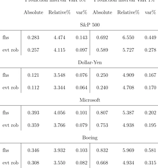
Table 15 shows absolute and relative average widths of ten days ahead VaR prediction intervals in the backtesting period. For all backtested assets and VaR confidence levels, evt rob has narrower prediction intervals than fhs, both in absolute and relative terms. Therefore, evt rob provides more accurate and reliable VaR predictions than fhs. For example, in S&P 500 and Boeing backtesting and for VaR forecasts at 1% level, classical FHS relative prediction intervals are about 14% and 21% larger than the ones for robust EVT.
In Table 15 the columns headed var% report average variances of daily changes in prediction intervals during the backtesting period. In all but one case, daily changes of evt rob prediction intervals have smaller variances than daily changes of fhs prediction intervals. For example, in S&P 500 and Boeing backtesting and for VaR forecasts at 1% level, such variances for evt rob are nearly 50% the ones for fhs. These results largely confirm the previous empirical findings that evt rob provides VaR predictions more stable over time than other methods. Overall, our robust procedure appears to control estimation risk in a better way than classical procedures and this induces more stable VaR profiles over time.
5
Conclusion
We propose a general approach to estimate conditional predictive distributions of asset returns based on robust semiparametric bootstrap methods for GARCH-type processes. Our approach adopts a robust estimator for parametric GARCH-type models and a robustified resampling method for standardized GARCH residuals. In the latter, a robust extreme value estimator controls the bootstrap instability deriving from influential observations in the tails of GARCH residual distributions. We show theoretically and by Monte Carlo simulation that to ensure ro-bustness of the whole bootstrap procedure both robustification steps are necessary. We apply this procedure to Value at Risk (VaR) predictions over different forecasting horizons. Monte Carlo simulation shows that our robust bootstrap procedure offers large improvements in accuracy of VaR predictions, especially for several days ahead horizons and in the presence of outlying or influential observations. In nearly all Monte Carlo experiments, our robust bootstrap procedure has lower mean square prediction errors, often by a large extent, and in contrast to classical meth-ods never fails validation tests at usual significance levels. Theoretical predictions of bootstrap breakdown points are confirmed by our simulations and non robust bootstrap procedures break down approximately at the calculated breakdown point. The simulation evidence is confirmed by the real data application. We backtest VaR prediction methods using S&P 500, Dollar-Yen, Microsoft and Boeing historical returns. For all VaR confidence levels and forecast horizons, only our robust bootstrap procedure never fails all validation tests at usual significance levels. When accounting for tail estimation error, our robust procedure provides more accurate and more stable over time VaR prediction intervals than other methods. Indeed, robust VaR prediction intervals can be almost 20% narrower and 50% less volatile than classical ones. Hence robust procedures allow to adapt outstanding risky positions to VaR limits more smoothly and thus more efficiently. Robust semiparametric bootstrap methods have applications beyond risk management. Future applications cover, for instance, robust bootstrap procedures for parametric estimators of
GARCH-type models or estimation of fund performance measures using bootstrap methods.
A
Proof of Proposition 1
Let η denote the fraction of outliers in the original sample of scaled innovations ˆz1, . . . ,zˆT. Then
it follows
PT(y⋆
T,T+h has at least one outlier ) = 1−(1−η)h.
By definition, ˆyα
T,T+h is theα-quantile ofFT,T⋆ +h. Therefore, ˆyαT,T+hbreaks down when a sufficiently
large proportion of simulated returns y⋆
T,T+h is corrupted, i.e. when
PT( y⋆
T,T+h has at least one outlier )≥α.
The probability on the left hand side gives the fraction of corrupted y⋆
T,T+h in the simulation.
When this fraction is larger than α, ˆyα
T,T+h breaks down. Therefore,
bα = arg min
η {1−(1−η)
h
≥α},
G au ss ia n in n ov at io n s ρ0 = 0 . 01 ρ1 = 0 . 01 α0 = 0 . 03 α1 = 0 . 02 α2 = 0 . 8 α3 = 0 . 2 E st im at or B ia s M S E B ia s M S E B ia s M S E B ia s M S E B ia s M S E B ia s M S E p m l 0. 01 05 0. 01 63 0. 02 53 0. 05 23 0. 06 31 0. 00 42 − 0. 15 89 0. 02 27 − 0. 05 29 0. 08 83 0. 01 98 0. 11 15 ro b a 0. 00 66 0. 01 65 0. 02 12 0. 05 61 0. 05 97 0. 00 43 − 0. 02 42 0. 02 37 − 0. 08 09 0. 08 94 − 0. 03 05 0. 11 30 ro b atr unc 0. 00 83 0. 01 70 0. 00 33 0. 05 72 0. 06 71 0. 00 43 0. 00 79 0. 02 41 − 0. 09 79 0. 09 18 − 0. 01 54 0. 11 50 S tu d en t t5 in n ov at io n s p m l − 0. 02 50 0. 01 46 − 0. 10 59 0. 06 96 0. 21 27 0. 01 23 0. 16 34 0. 05 47 − 0. 94 15 0. 23 70 0. 26 69 0. 32 64 ro b a − 0. 03 41 0. 01 34 − 0. 14 26 0. 05 83 0. 08 34 0. 00 67 − 0. 34 21 0. 02 32 − 0. 75 73 0. 16 02 − 0. 65 77 0. 20 69 ro b atr unc − 0. 03 49 0. 01 35 − 0. 14 27 0. 05 85 0. 08 01 0. 00 70 − 0. 31 58 0. 02 38 − 0. 69 68 0. 17 71 − 0. 68 28 0. 22 03 L ap la ce in n ov at io n s p m l − 0. 02 63 0. 01 41 − 0. 11 63 0. 06 81 0. 16 09 0. 00 76 0. 01 21 0. 03 08 − 0. 67 08 0. 17 06 0. 25 65 0. 24 52 ro b a − 0. 03 37 0. 01 35 − 0. 14 33 0. 05 89 0. 12 87 0. 00 71 − 0. 43 53 0. 02 52 − 0. 66 74 0. 16 73 − 0. 29 96 0. 22 57 ro b atr unc − 0. 03 73 0. 01 36 − 0. 14 59 0. 05 97 0. 12 78 0. 00 66 − 0. 39 37 0. 02 52 − 0. 64 57 0. 16 90 − 0. 28 61 0. 23 50 R ep la ce -i n n ov at iv e m o d el p m l 0. 42 25 0. 09 37 − 0. 45 64 0. 46 12 3. 94 89 0. 64 84 4. 98 75 2. 18 03 − 4. 63 13 2. 78 12 3. 80 14 5. 88 39 ro b a 0. 00 15 0. 01 84 0. 05 78 0. 06 10 1. 04 72 0. 04 89 1. 23 85 0. 21 52 − 1. 19 21 0. 38 71 0. 89 78 0. 89 34 ro b atr unc 0. 00 33 0. 01 86 0. 04 47 0. 06 19 1. 06 40 0. 05 16 1. 29 70 0. 23 27 − 1. 17 35 0. 42 97 0. 91 11 0. 92 84 T ab le 1: P er ce n ta ge b ia s an d M S E of est im at ed p ar am et er s of th e A R (1 ), as ym m et ri c G A R C H (1 ,1 ) m o d el (7 )– (8 ).