Graduate Theses and Dissertations Iowa State University Capstones, Theses and Dissertations 2016
Image analysis and machine learning based
methods for disease detection in soybeans
Hsiang Sing NaikIowa State University
Follow this and additional works at:https://lib.dr.iastate.edu/etd Part of theMechanical Engineering Commons
This Thesis is brought to you for free and open access by the Iowa State University Capstones, Theses and Dissertations at Iowa State University Digital Repository. It has been accepted for inclusion in Graduate Theses and Dissertations by an authorized administrator of Iowa State University Digital Repository. For more information, please [email protected].
Recommended Citation
Naik, Hsiang Sing, "Image analysis and machine learning based methods for disease detection in soybeans" (2016).Graduate Theses and Dissertations. 15981.
Image analysis and machine learning based methods for disease detection in soybeans
by
Hsiang Sing Naik
A thesis submitted to the graduate faculty
in partial fulfillment of the requirements for the degree of MASTER OF SCIENCE
Major: Mechanical Engineering Program of Study Committee:
Baskar Ganapathysubramanian, Major Professor Soumik Sarkar
Arti Singh
Iowa State University Ames, Iowa
2016
ii
DEDICATION
For Joanna,
For Papa and Mama, For the three little angels, And the Woodstock folks.
iii
TABLE OF CONTENTS
Page
ACKNOWLEDGMENTS ... iv
ABSTRACT………. ... v
CHAPTER 1. GENERAL INTRODUCTION ... 1
Background ... 1
Thesis Organization ... 3
CHAPTER 2. A REAL-TIME PHENOTYPING FRAMEWORK USING MACHINE LEARNING FOR PLANT STRESS SEVERITY RATING IN SOYBEAN ... 4
Abstract ... 4
Introduction ... 5
Materials and Methods ... 9
Genetic material and field phenotyping ... 9
Image acquisition ... 10
Dataset description ... 10
Variables Description... 11
Preprocessing ... 11
Feature extraction from expert elicitation ... 13
Classification... 14
Overview of classification algorithms ... 18
Hierarchical classification ... 20
Results and Discussion ... 23
Population Canopy Graph ... 25
Model selection ... 26
Cellphone App and PC Software ... 26
Conclusion ... 28
References ... 29
Appendix. Standard imaging protocol ... 31
iv
ACKNOWLEDGMENTS
I would like to express my gratitude to a few great minds who were great influence and help towards the completion of this research and thesis.
To start things off, I would like to thank Dr. Baskar Ganapathysubramanian, my major professor. He was willing to accept me into his research group as an undergraduate student and introduced me to the amazing world of programming, image processing and machine learning. The door to his office was always open whenever I had questions on research or other matters. He is not only a great mentor and a teacher, but a great friend and was a great father-figure for me when I was in need of one, and for this I am forever grateful.
Next, I would like to express my thanks to Dr. Soumik Sarkar, Dr. Asheesh Singh and Dr. Arti Singh, who are all experts in their line of research and were very much involved in this research. Without their passionate participation and input, this research could not have been completed.
I would also like to acknowledge the brilliant people from Dr. Singh’s group, Jiaoping Zhang, Teshale Assefa, Sarah Jones, Brian Scott, and Jae Brungardt. They were instrumental in the collection of images and put in lots of hours of hard work for the success of this research.
Furthermore, I would like to thank everyone from the Plant Sciences subgroup, Nigel, Vahid, Vikas, Zaki and Alec, for their constant support, crazy yet brilliant ideas, and their persistent attitude at attacking a problem. We have done great work together.
Last but not least, I would like to express my profound gratitude to my parents, and my girlfriend, for providing me with unfailing support and continuous encouragement throughout my years of study and through the process of researching and writing this thesis. This accomplishment would not have been possible without them. Thank you.
v
ABSTRACT
Plant phenotyping is important for genetic enhancements and plant biology research. There is a lot of work done to improve yield of crop plants, by selecting good genotypes to cross-breed in an effort to curb diseases or genetic deficiencies in these crops. In order to select these genotypes, one would have to perform phenotyping. Currently, plant phenotyping is based on visual assessment, where a breeder or researcher would have to visually inspect each plant and visually rate them. Visual rating is inefficient and can be inconsistent due to intra-rater repeatability or inter-rater reliability issues leading to incorrect visual scores. Not only that, it is also labor intensive and time consuming. Hence, there is a need to develop new tools amenable to high throughput phenotyping (HTP) for large scale plant genotype assessments. This requirement for high throughput phenotyping is applicable in a variety abiotic and biotic stresses.
We developed a HTP framework which utilizes digital images in an effort for disease detection. This framework enabled us to accurately assign disease ratings to soybean plants that were affected by iron deficiency chlorosis (IDC). Utilizing image analysis techniques, we successfully extracted features pertaining to IDC and trained classification models on these features. A hierarchical classifier, based on linear discriminant analysis and support vector machine classifiers, produced the highest accuracy of 96%. Also, this framework was successfully implemented as a cellphone app. We envision to utilize hyperspectral imaging in the future for more accurate disease detection, prior to symptoms being visible.
1
CHAPTER 1
GENERAL INTRODUCTION Background
Detection and diagnosis of diseases is an important aspect to plant breeders and pathologists. Plant diseases have a profound effect on harvested yield, and subsequently the economy. There have been various efforts to breed different crop plant genotypes with improved disease tolerance to curb the impact of diseases. To identify the right genotypes, one would have to perform phenotyping. In addition, plant phenotyping is important for genetic enhancements and plant biology research.
Currently, common plant phenotyping is based on visual assessment, where a breeder or researcher would have to visually inspect individual plants and assign disease ratings. While visual rating may be the current standard, it has it shortcomings. Visual rating is not only time consuming, where one would have to spend days visually rating a plot of land, but is also labor intensive and inefficient. To add to that, visual rating can be inconsistent due to intra-rater repeatability or inter-rater reliability issues, leading to incorrect or varying visual scores, less accuracy and reproducibility. Also, it is crucial to rate hundreds or thousands of plots within a short time frame to minimize plant stage variability.
Hence, there is a need to develop new tools amenable to high throughput phenotyping (HTP) for large scale plant genotype assessments that is rapid, cheap, accurate, and unbiased. Since phenotyping are done at different stages of a plant’s growth, repeated measurements with high accuracy can help in identifying right genes controlling disease in soybeans.
2
Driven by these requirements, we proposed a simple framework that extracts features that are known to quantify the extent of specific diseases from digital images. There are several advantages of using digital images compared to visual rating. Digital images can store significantly more information compared to simple numerical ratings, while also allowing for plant breeders and pathologists to better allocate their time, by spending more time analyzing data instead of using the bulk of their time for data collection. Also, digital image collection need not be done by professionals in the field, hence allowing for collection to be done simultaneously by multiple individuals.
The primary goal of the present study is to develop a disease detection framework that is applicable on soybeans using machine learning and image analysis techniques. Soybeans are a very important part of the economy, with annual revenue of $40 billion in the USA alone. Hundreds of millions of dollars are being lost due to diseases in soybeans, hence the motivation for this study. Utilizing machine learning and image analysis techniques, disease detection frameworks can be developed for a variety of diseases through digital images. Chapter 2 of this thesis describes how we utilized these methods to develop a disease detection framework for iron deficiency chlorosis in soybeans. Future targets for this study would be to utilize hyperspectral imaging, which enables for disease to be detected even before visible symptoms appear on the surface of leaves, and allows for rapid, high throughput phenotyping.
3
Thesis Organization
This thesis follows the journal paper format. Chapter 1 includes the general introduction to the thesis. Chapter 2 is a modified version of the paper that was submitted to Plant Methods. Chapter 3 comprises general conclusions from the journal paper.
4
CHAPTER 2
A REAL-TIME PHENOTYPING FRAMEWORK USING MACHINE LEARNING FOR PLANT STRESS SEVERITY RATING IN SOYBEAN
Modified from a paper submitted to Plant Methods
Hsiang Sing Naik, Jiaoping Zhang, Alec Lofquist, Teshale Assefa, Soumik Sarkar, David Ackerman, Arti Singh, Asheesh K Singh, Baskar Ganapathysubramanian
Abstract
Background: Phenotyping is a critical component of plant research. Accurate and precise trait collection, when integrated with genetic tools, can greatly accelerate the rate of genetic gain in crop improvement. However, efficient and automatic phenotyping of traits across large populations is a challenge; which is further exacerbated by the necessity of sampling multiple environments and growing replicated trials. A promising approach is to leverage current advances in imaging technology, data analytics and machine learning to enable automated and fast phenotyping and subsequent decision support. In this context, the workflow for phenotyping (image capture → data storage and curation → trait extraction → machine learning/ classification → models/apps for decision support) has to be carefully designed and efficiently executed to minimize resource usage and maximize utility. We illustrate such an end-to-end phenotyping workflow for the case of plant stress severity phenotyping in soybean, with a specific focus on the rapid and automatic assessment of Iron Deficiency Chlorosis (IDC) severity
5
on thousands of field plots. We showcase this analytics framework by extracting IDC features from a set of ~ 4500 unique canopies representing a diverse germplasm base that have different levels of IDC, and subsequently training a variety of classification models to predict plant stress severity. The best classifier is then deployed as a smartphone app for rapid and real time severity rating in the field.
Results: We investigated 10 different classification approaches, with the best classifier being a hierarchical classifier with a mean per-class accuracy of ~96%. We construct a phenotypically meaningful ‘Population Canopy Graph (PCG)’, connecting the automatically extracted canopy trait features with plant stress severity rating. We incorporated this image capture → image processing → classification workflow into a smartphone app that enables automated real-time evaluation of IDC scores using digital images of the canopy.
Conclusion: We expect this high-throughput framework to help increase the rate of genetic gain by providing a robust extendable framework for other abiotic and biotic stresses. We further envision this workflow embedded onto a high throughput phenotyping ground vehicle and unmanned aerial system (UAS) that will allow real-time, automated stress trait detection and quantification for plant research, breeding and stress scouting applications.
Introduction
Soybean (Glycine max (L.) Merr.) is a huge source of revenue for the United States, with production of approximately USD 40 billion in 2014[1]. There are various factors that affect soybean yield, such as nutrient availability, weed management,
6
genetics, row configuration, stress (biotic and abiotic) and soil fertility [2]. Iron Deficiency Chlorosis (IDC) is a yield-limiting abiotic stress which affects plants that usually grow on calcareous soil with high pH. Soybean plants growing in calcareous soils (soils with free calcium carbonate and high pH) are unable to uptake iron from the soil leading to iron deficiency in plants. IDC causes reduced plant growth leading to a reduction in yield potential and quality of the crop. In the mid-west USA, IDC is one of the major problems reducing soybean yield, by as much as 20% for each visual rating point [3]. This causes an estimated economic loss of $ 260 million in 2012 alone[4]. IDC symptoms are observed at early plant growth stages on newly grown leaf tissue where chlorosis (yellowing) occurs in between the veins of the leaves, while the veins themselves remain green [5]. The extent of the problem varies depending on the cultivar, field and the year.
Soybean breeders in US breed for genotypes with improved IDC tolerance by selecting for genes that help make the plant more iron uptake efficient [6]. Selection for desirable soybean genotype (with IDC tolerance) is done either through phenotyping in the field or in greenhouses [7], or genotyping with molecular markers linked to genes that improve IDC tolerance. More than 10 genes have been reported to be associated with improving IDC tolerance [8,9] making genotyping approaches onerous where a breeding program may be working to select for several other traits. Phenotyping is most suitable as it allows identification of soybean genotypes that have an acceptable IDC tolerance. Furthermore, this method is cost effective and potentially requires little access to specialized labs.
7
Current methods for phenotypically measuring IDC are completely visual and labor-intensive. Cianzo et al.[3] and Froehlich and Fehr[7] reported that visual scoring is the simplest, subjective measurement that requires relatively less labor. However, it has reduced accuracy if the evaluation is made in diverse environments and by different raters [10]. In addition, there can be intra-rater repeatability or inter-rater reliability [11] issues leading to incorrect visual scores. It also depends on the subjectivity (and its variability) of the IDC rater. Specifically, the human eye can get tired after long hours of scoring plants for various traits, which can produce large intra-rater variability in rating scores, thus resulting in diminished accuracy and reproducibility. In a breeding program, hundreds or thousands of plots are rated in a short time frame. A short time frame is crucial because one has to minimize plant stage variability, i.e., variability that is introduced if genotypes are rated over a longer time frame. It is therefore essential to develop methods that allow for unbiased, accurate, cost effective and rapid assessment for IDC in particular, and plant biotic (e.g., diseases) and abiotic stresses in general. There has been recent work in this regard to design, develop and deploy high efficiency methods/tools to quantify leaf surface damage [12] as well as plants response to pathogens [13]. Additionally, a number of approaches using imaging methods for phenotyping, such as fluorescence and spectroscopic imaging have been successful for stress-based phenotyping [14], high throughput machine vision systems that use image analysis for phenotyping Arabidopsis thaliana seedlings [15] and barley [16], hyperspectral imaging for drought stress identification in cereal [17], and a combination of digital and thermal imaging for detecting regions in spinach canopies that respond to soil moisture deficit [18] which have proven to be successful. However, a simple, user
8
friendly framework is unavailable for the public to phenotype for IDC in soybean plants. The availability of a simple modular approach could potentially be generalized for phenotyping of multiple stresses.
Motivated by these reasons, we developed a simple framework (image capture → data storage and curation → trait extraction → machine learning/ classification → models/ smartphone apps for decision support) that extracts features that are known to quantify the extent of IDC (amount of yellowing, amount of browning) from digital images. To determine a relationship between these features and their respective ratings, we employed a host of machine learning techniques, further elaborated in the latter stages of this paper, to perform supervised classification. Subsequently, using information obtained from these classifiers, a physically meaningful population canopy graph (PCG) connecting the features with the visual IDC rating was constructed for a diverse soybean germplasm. This complete framework, which is based on fast feature extraction and classification, can then be used as a high throughput phenotyping (HTP) system for real time classification of IDC. We enable real time phenotyping by implementing the software framework as a GUI-based, user-friendly software that is also deployed on smartphones. This step successfully abstracts the end-user from the mathematical intricacies involved, thus enabling widespread use. We showcase this software framework by extracting IDC features (amount of yellowing, amount of browning) from a set of 4366 plants that have different IDC resistances.
We envision our classifier based framework as a modular, extensible and accurate phenotyping platform for plant researchers including breeders and biologists.
9
Materials and Methods Genetic material and field phenotyping
A total of 478 soybean genotypes, including 3 maturity checks and 475 soybean plant introduction (PI) lines acquired from the USDA soybean germplasm collection, were planted in the Bruner farm in Ames, IA, 2015, where soybean IDC was present in previous years. The design for this field experiment follows a randomized complete block design, with a total of four replications. Each PI line was planted once per replication, while the IDC checks (two) and maturity checks (three) were repeated at regular intervals in the field with four plots per replication. At two soybean growth stages [19]: the second to third trifoliate (V2-V3) and fifth to sixth trifoliate (V5-V6) leaf stages, the soil pH was tested in the Soil and Plant Analysis Laboratory, Iowa State University. At each stage, eight soil samples were randomly collected from each replication and were mixed as one test sample. The soil pH values ranged at 7.80 - 7.95 and 7.75 - 7.85 at V2-V3 and V5-V6 growth stages, respectively. Field visual ratings (FVR) of IDC severity by expert phenotypers were collected at V2-V3 and V5-V6 growth stages, as well as two weeks after the V5-V6 stage to obtain soybean canopies with a variety of IDC expression. FVR was done on a scale of 1 to 5 described by Lin et al., where 1 indicates no chlorosis and plants were normal green; 2 indicates plants with modest yellowing of upper leaves; 3 indicates plants with interveinal chlorosis in the upper leaves but no stunting growth; 4 indicates plants are showing interveinal chlorosis with stunting growth; and 5 indicates plants show severe chlorosis plus stunted growth and necrosis in the new youngest leaves and growing points [20].
10 Image acquisition
We utilized a Canon EOS REBEL T5i camera for image acquisition. Images were stored in the native RAW format. Substantial effort was put in to develop a standard imaging protocol (SIP) (Additional file 1) to ensure imaging consistency and quality. The flash function was kept off and an umbrella was always used to shade the area under the camera view in order to minimize illumination discrepancies between images. A light/color calibration protocol was also followed. An image of an X-Rite ColorChecker Color Rendition Chart was taken at the beginning of imaging operations, and every 20 min thereafter or whenever light condition changes (cloud cover, etc.). As the appearance of color is affected by lighting conditions, using the X-Rite ColorChecker Color Rendition Chart enables color correction to be applied to ensure that colors are uniform throughout all the plant canopy images collected at that moment. When taking pictures, the whole canopy was fit in the field of view of the camera. Whenever possible, weeds and other plant residuals that connect to the plant canopy in the view of camera were removed for enhanced efficiency of subsequent image processing.
Dataset Description
A total of 5916 RGB (493 plots including PI accessions and checks x 4 replications x 3 time points) images were acquired, along with subsequent FVR. Each time point consists of four repetitions for a total of 1972 (493x4) images, with 493 images per repetition. Image acquisition at each of these time points was vital to obtain a large variety of IDC symptoms, as IDC symptoms progress in time. The idea was to develop a dataset with similar number of observations per IDC rating. This was, however,
11
not possible simply due to the fact that a large fraction of plants remained healthy (FVR = 1) throughout the image acquisition period. Following image acquisition, for quality control, each image was inspected visually, and those that did not adhere to the SIP were removed, which resulted in 4366 images in the remaining image set.
Variables Description Preprocessing
Segmentation: Each image was converted from native Red, Green, Blue (RGB) format to HSV (Hue, Saturation, Value) format to efficiently perform background removal, leaving only the plant canopy (foreground). Hue is defined as the color or tint of an object, with values ranging from 0° to 359°, whereas saturation is defined as the range of gray in the color space (0% to 100%) [21]. The background of an image (soil, debris) contains more gray pixels compared to the foreground (plant), and lacks green and yellow hue values; therefore, most of the background was removed by excluding pixels that had saturation value below a predefined threshold and hue values outside of a predefined range. The saturation threshold value was obtained by identifying the saturation values of the background in 148 diverse images. The hue range was simply obtained from the hue color wheel, removing pixels that were neither green nor brown. This combined thresholding based on incorporating hue thresholding with saturation thresholding ensured a reliable and robust segmentation process.
Noise and outlier removal: Once segmentation was done, the connected components method [22] was used on the processed image to remove spurious outliers and noise from the image, (for example, plant debris on soil). This was accomplished by
12
identifying clusters of pixels which are connected to one another, labelling them, and identifying the largest connected component. Since the imaging protocol was designed to ensure that the plant was centered in the imaging window and in the foreground, it follows that the largest connected component is invariably the plant. Cleaning was done by removing any other connected components that contain fewer pixels than the largest connected component. Then, a mask of the isolated plant was applied onto the original RGB image in order to display the isolated plant in color. No significant pixel loss was observed which is common in other thresholding methods [23]. The use of the connected components approach to isolate plants from background is extremely fast and accurate. In conjunction with a SIP, using connected components for preprocessing is very promising, especially for near real time phenotyping applications. The preprocessing sequence is illustrated in Figure 1.
Figure 1. Image preprocessing sequence from original image of canopy to completed automated pre-processed field soybean canopies.
13 Feature extraction from expert elicitation
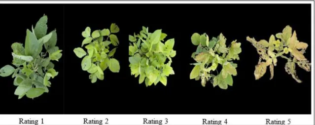
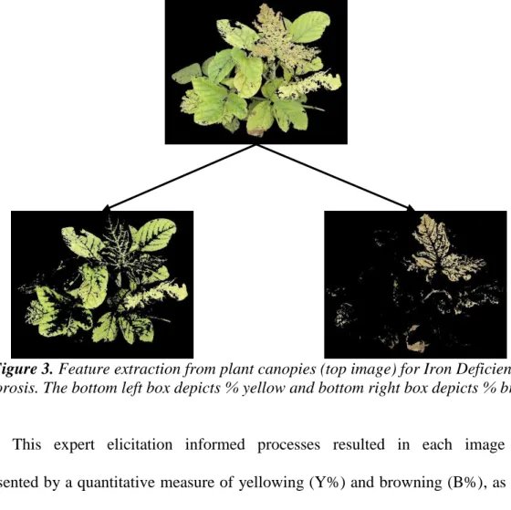
Field visual ratings are assigned based on the extent of chlorosis (yellowing) and necrosis (browning) expressed on the canopy, as described earlier and illustrated in Figure 2. Elicitation from domain knowledge experts (i.e., phenotypers) suggested that color signatures (green to yellow to brown), specifically extent of (dis)coloration (chlorosis → yellowing, and necrosis → browning) were viable predictors to quantify IDC expression. Each pixel of the processed image belonging to the canopy was identified as either green, yellow, or brown through respective hue values, and the extent of discoloration from green was represented in the form of the percentage of canopy area that experience these visual changes (Y% and B%), as seen in Figure 3.
Figure 2. Iron Deficiency Chlorosis severity description using a field visual rating scale of 1 – 5.
14
Figure 3. Feature extraction from plant canopies (top image) for Iron Deficiency Chlorosis. The bottom left box depicts % yellow and bottom right box depicts % brown.
This expert elicitation informed processes resulted in each image being represented by a quantitative measure of yellowing (Y%) and browning (B%), as shown in Equation 1.
Classification
In order to map these quantitative variables to the visually rated IDC ratings, we utilize several state of the art machine learning algorithms to construct classification models. The field visual rating served as the categorical output variable (classes) while the inputs were the 2-tuple (Y%, B%). The classification models are then eventually used to generate IDC ratings given different input variables.
The total dataset consisted of 4366 images following quality control as detailed in the Dataset Description section. The images were sorted into 5 groups which correspond
15
to their respective FVR, with majority of the observations falling into group 1 (FVR = 1). The remaining groups (FVR = 2/3/4/5) meanwhile contained a balanced distribution of observations amongst themselves.
Due to the imbalanced nature of the dataset with a preponderance of images belonging to FVR 1, two variations of the dataset were used to develop classification models: a) Using observations from time point 2 and b) for a combination of time point 1, 2, and 3. Time point 2 served as a standalone dataset due to the fact that it has the largest distribution of observations containing each of the FVRs. We utilized several classification algorithms, namely classification trees (CT), random forests (RF), Naïve Bayes (NB), linear discriminant analysis (LDA), quadratic discriminant analysis (QDA), multi-class support vector machines (SVM), k-nearest neighbors (KNN), and Gaussian mixture models (GMM). Building upon the results, we subsequently utilized the concept of hierarchical classification to develop two additional models using a combination of LDA and SVM algorithms.
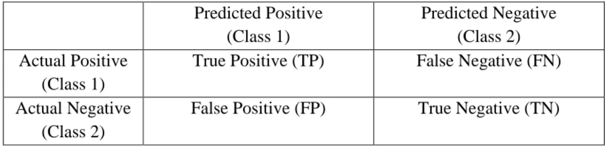
The dataset was randomly sampled into two subsets in a 75%-25% ratio. The larger subset (75%) served as the training set, while the remaining subset served as the testing dataset (25%). The training dataset is used to train the classifier, by learning a mapping of the Y% and B% with their expected IDC ratings. Subsequently, the testing dataset is used to estimate the performance of the classification model, by applying it on the testing dataset to classify each observation. The performance of the classifier can be interpreted from the confusion matrix (Table 1). The diagonals on a confusion matrix show the number of observations where, the predicted rating is equal to the actual rating, whereas the off-diagonal elements are observations that have been misclassified.
16
An example confusion matrix for a binary classification problem is shown below: Table 1: Confusion matrix
Predicted Positive (Class 1) Predicted Negative (Class 2) Actual Positive (Class 1)
True Positive (TP) False Negative (FN) Actual Negative
(Class 2)
False Positive (FP) True Negative (TN)
Three measures of accuracy of the classifier are reported from the confusion matrix: a) Accuracy which quantifies the fraction of the training dataset that is correctly
predicted.
Equation 2
b) Per-class accuracy is a more refined metric which calculates how the classifier performs for each of the classes. This is useful when the instances in each class vary a lot, i.e., when the classes are imbalanced (as is the case in this work), since accuracy is usually overestimated due to the impact of the class with the most instances dominating the accuracy statistic.
Equation 3
i = 1,…,n, where n = number of classes.
c) Mean per-class accuracy (MPCA) is the mean per-class accuracy over these classes.
17
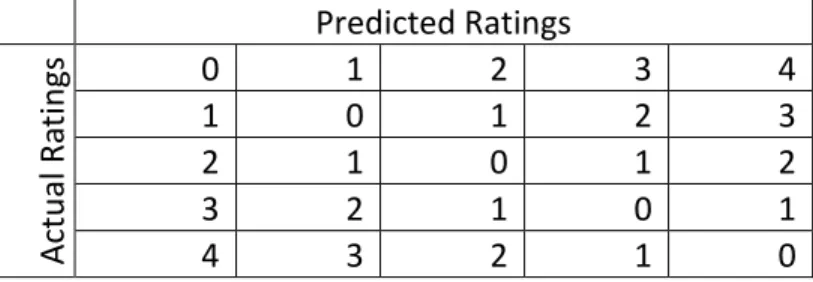
In addition, we compute the misclassification costs in order to quantify the cost of the misclassification errors – i.e., if an observation in rating 1 were to be classified as rating 5, it would have a higher misclassification cost than if it were to be classified as rating 2. Essentially, calculating the misclassification cost enables us to know, if errors are made, how bad the errors are. To do so, we defined a misclassification cost matrix, as detailed in Table 2. The off-diagonals of the matrix are the misclassification cost for each of the ratings, which are finite, real values [24]. For example, if the actual rating of an observation is rating 1, the error of misclassifying the observation to rating 5 is 4 times as costly as misclassifying the observation to rating 2, and so on. Then, misclassification cost is computed using Equation 5.
Table 2: Cost matrix, wij
Predicted Ratings Act u al Ra tin gs 0 1 2 3 4 1 0 1 2 3 2 1 0 1 2 3 2 1 0 1 4 3 2 1 0 Equation 5 ,
18
= confusion matrix = cost matrix = number of observations
Lastly, we employ cross-validation to estimate the average generalization error for each classifier. Cross-validation essentially is a method of assessing the accuracy and validity of a statistical model for generalization on future datasets. From a generalizability standpoint, the absolute accuracy of a classifier is less important as it could be subject to bias and overfitting. Hence, cross-validation is a method of performance estimation based on the variance. The ideal estimation method would have low bias and low variance [25]. We used k-fold cross-validation, with k = 10 which is a good compromise between variance and bias[25]. K-fold CV was repeated 10 times to compute the mean cross-validation misclassification error for each model. While accuracy and MPCA detail the performance of a classifier on essentially the same dataset, mean cross-validation misclassification error provides information on how well the classifier performs on other datasets.
Overview of classification algorithms
We briefly describe each of the classification algorithms [26]. We refer the interested reader to a more detailed description of these methods in [27, 28,29].
Decision Trees: It is based on the construction of predictive models with a tree-like structure that correlates observations to their corresponding categories such as classes (for classification) and rewards (for decision-making problems). These observations are sorted down the tree from the root to a leaf node, which in turn classifies
19
the observation. Decision Trees perform well on lower dimensional classification problems, but tend to falter when the dimension of the classes increases.
Random Forests: An ensemble method employed to regularize the greedy, heuristics nature of the decision tree training which sometimes causes overfitting. This method combines results and structures from a number of trees prior to coming to a conclusion. Multiple trees are grown from random sampling of the data. Nodes and branch choices of a tree are also determined through a non-deterministic manner. These models are more robust to uncertainties.
Naïve Bayes: A supervised classification technique for constructing classifiers of a probabilistic graphical model. It is based on the assumption that each feature is independent of each other. Naïve Bayes have been used in a variety of fields, and is a popular method for text categorization.
Linear Discriminant Analysis (LDA): A linear classification technique based on the idea of Fisher’s Metric, with an aim to maximize between class variance, while minimizing within-class variance. This allows the linear combination of features to improve separability among two or more classes. This requires an assumption of equal variance-covariance matrices of the classes.
Quadratic Discriminant Analysis (QDA): A modification of Linear Discriminant Analysis, except a covariance matrix must be estimated for each class. This allows overcoming the problem where the variance-covariance differs substantially, where LDA will not perform well.
Support Vector Machine (SVM): The most popular among supervised, discriminative kernel-based methods for classification. SVM uses kernel functions to
20
project data into a higher dimensional space in order to separate data from different classes which cannot be linearly separated. A hyperplane is constructed to determine the bounds in which each class is separated, to maximize class separability.
K-Nearest Neighbors (KNN): A non-parametric classification method. This algorithm assigns the same class label to data samples as its k nearest neighbors based on a similarity metric defined on the feature space, where k is an integer. This nonlinear algorithm works reasonably well for multi-class classification problems.
Gaussian Mixture Model (GMM): A generative, unsupervised data model that aims to identify a set of Gaussian distributions mixtures which best describe the data. GMM is a probabilistic technique where every data example is expressed as a sample of the distribution which is a weighted sum of k Gaussian distribution. Once this model is created, a Bayes classifier is applied in attempt to solve classification problems.
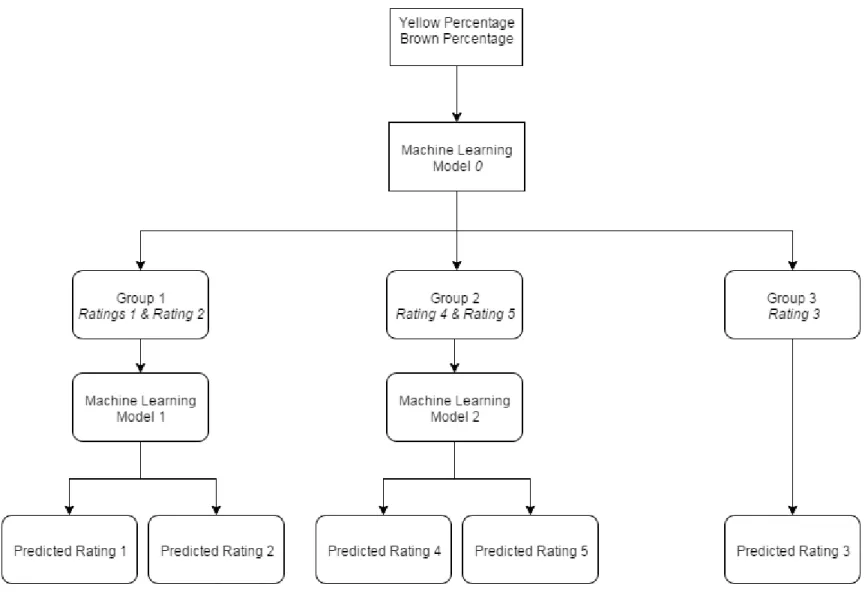
Hierarchical classification
We subsequently pursued a hierarchical classification strategy that is motivated by expert elicitation of information about IDC susceptibility. Hierarchical classification is known to work well on datasets with a larger number of classes but with fewer observations. The IDC data set fell into this category. Also, the task of designing the hierarchy in this classification strategy enables the inclusion of expert knowledge. Here, the hierarchical structure is predefined, based on insight and existing knowledge of class hierarchies, which then contributes to improving classification accuracy.
In this case, the hierarchies were identified based on the susceptibility of the genotypes to IDC. Specifically, rating 1 and 2 are usually taken together as low
21
susceptibility genotypes, while rating 4 and 5 are taken together as high susceptibility genotypes. We thus designed a two-step classification strategy: In Step A, a classifier is learnt that can separate the data into low, medium and high susceptibility groups. Step B then further classifies these groups into rating 1 or 2 (for the low susceptibility group), and rating 4 or 5 (for the high susceptibility group).
For Step A, we deploy both LDA and multi-class SVMs. The learnt classifier is called Model 0, to classify the dataset into three groups (low, medium and high susceptibility) based on their yellow and brown percentage. For Step B, we deploy Support Vector Machine as the classification is binary. Figure 4 displays a flowchart of this hierarchical classifier.
22
Figure 4. Hierarchical classification workflow
2
23
Results and Discussion
A number of classification algorithms were capable of achieving high mean per class accuracy, more than 90%, for classification on the time point 2 data set. Hierarchical models performed relatively well, with a mean per class accuracy at 95.9%. More importantly, when the classifier made incorrect predictions, the results were predominantly within the same susceptibility class - i.e., an error in rating 1 typically falls to rating 2, and not into rating 5 etc. This is illustrated in the misclassification cost metric for each classifier, as detailed in Equation 5. The best performing classifier, classification trees, were able to correctly predict new observations 100% of the time.
When data from all time points were used to train and test a classifier, the hierarchical model performed the best, with 91% accuracy. Other classifiers fell short of the 90% mark. The decrease in accuracy was expected simply because combining all three time points caused the data set to be more imbalanced that before.
While being able to have high classification accuracy is important, the capability of a classifier to produce an interpretable PCG was extremely vital. This is quantified by the
interpretability of the PCG, and is further discussed in the PCG and Model Selection sections. The results of each of the classification models are displayed in Tables 3 and 4.
24
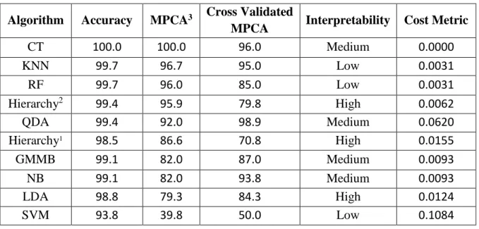
Table 3: Results for machine learning algorithm model accuracies developed using a sub-set of Iron Deficiency Chlorosis data on a diverse set of soybean accessions.
Algorithm Accuracy MPCA3 Cross Validated
MPCA Interpretability Cost Metric
CT 100.0 100.0 96.0 Medium 0.0000 KNN 99.7 96.7 95.0 Low 0.0031 RF 99.7 96.0 85.0 Low 0.0031 Hierarchy2 99.4 95.9 79.8 High 0.0062 QDA 99.4 92.0 98.9 Medium 0.0620 Hierarchy1 98.5 86.6 70.8 High 0.0155 GMMB 99.1 82.0 87.0 Medium 0.0093 NB 99.1 82.0 93.8 Medium 0.0093 LDA 98.8 79.3 84.3 High 0.0124 SVM 93.8 39.8 50.0 Low 0.1084
Table 4: Results for machine learning algorithm model accuracies developed using the complete set of Iron Deficiency Chlorosis data on a diverse set of soybean accessions.
Algorithm Accuracy MPCA3 Cross Validated
MPCA Interpretability Cost Metric
CT 99.7 91.7 78.4 Low 0.0027 Hierarchy2 99.2 90.7 79.2 High 0.0082 Hierarchy1 98.3 84.0 79.0 High 0.0201 QDA 98.5 83.2 77.9 Medium 0.0201 NB 98.4 79.0 78.5 Medium 0.0284 KNN 99.5 75.8 84.3 Low 0.0073 RF 99.1 75.0 81.1 Low 0.0092 GMMB 99.4 74.2 82.7 Low 0.0064 LDA 98.5 71.7 76.9 High 0.0156 SVM 97.3 45.8 45.3 Low 0.0458 1 LDA and SVM 2 SVM and SVM
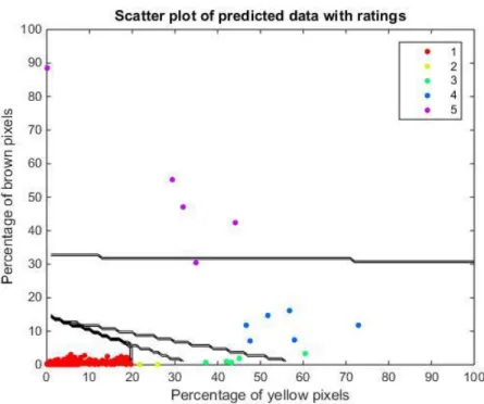
25 Population Canopy Graph
It was interesting to note that the learnt classifier revealed insightful phenotypic intuition. Specifically, we queried the classifier to predict ratings for a uniform sampling of the Y% and B% range. This data is then used to construct a 2D plot that depicts decision boundaries that separate various IDC classes, referred to as a PCG. This graph, shown in
Figure 5 which displays the PCG output from Hierarchy2 classification results on the test set, correlates very well with expert intuition. For example, Ratings 1-3 exhibit low brown values (corresponding to minimal to no necrosis), while ratings 4 and 5 have much higher brown values (corresponding to significant necrosis and/or chlorosis and necrosis). Moreover, PCGs with linear decision boundaries were preferred owing to better interpretability (see Model Selection section).
Figure 5: Population Canopy Graph of predicted data using a testing set with images and visual rating for IDC in soybean.
26 Model selection
Based on information about accuracy, MPCA, cross-validated MPCA, and interpretability of the PCG, a model selection table was constructed to summarize each model. Interpretability of the model is based on whether the decision boundaries made physical sense to the plant researcher, and was scored either ‘Low’, ‘Medium’, or ‘High’; ‘Low’ for models that did not correlate with expert intuition (e.g.: individual islands, quadratic boundaries that appear to be biased), ‘Medium’ for models that partially correlates with expert intuition, and ‘High’ for models that correlated well with expert intuition.
The ideal model would: 1) Have high MPCA, 2) High cross-validated MPCA, and 3) High interpretability. Interpretability was the criteria with the highest importance; hence models with high MPCA and cross-validated MPCA but with subpar interpretability were not taken into consideration. The hierarchical model Hierarchy2 had the best trade-offs amongst these criterions, as shown in Tables 3 & 4, and was chosen as the best model.
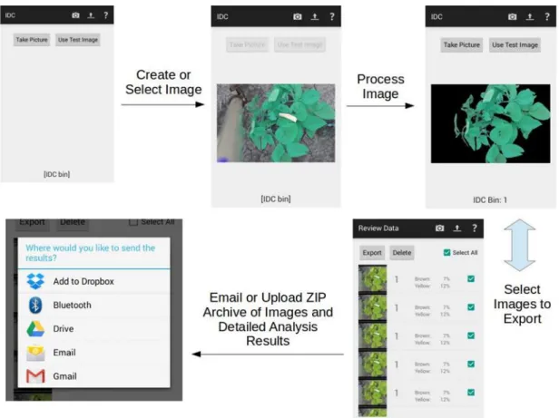
Cellphone App and PC Software
To enable high throughput phenotyping using the developed classifier, we embed the preprocessing stage as well as the classifier into an easy to use GUI that is deployable as a smartphone app. This app is supported on all Android-based devices, such as tablets and smartphones and has the full functionality of the desktop-based version. The Android-based app allows users to take pictures with their devices and extract the IDC rating in real time. This allows for portability and instant acquisition of data. Figure 6 shows a flowchart of illustrating the app. When the app is launched, the user has a choice between taking a new picture, and analyzing a picture already contained in the device. Once a picture has been selected, it is processed and the IDC score evaluated and displayed on the screen. The user
27
can export single or multiple images in tabular form through various methods, such as Dropbox, Bluetooth, Google Drive, and through email. This app allows untrained personnel and/or unmanned ground vehicles to extract and transmit IDC ratings without the need for a trained plant researcher/phenotyper looking at every plant. This is a tremendous enabler in terms of dramatically increasing the number of plants that can be accessed. In addition to the smartphone based app, a desktop based GUI will also be released to enable batch processing of a large number of images. This allows offline (or off site) analysis of images that are either captured manually or in an automated fashion.
Figure 6: Smartphone app flowchart demonstrating the integration of pre-processing, machine learning enabled classification and iron deficiency chlorosis visual rating in real time.
28
We designed, developed and deployed an end-to-end integrated phenotyping work-flow that enables fast, accurate and efficient plant stress phenotyping. We show how image processing and machine learning can be deployed to construct classifiers that can automatically evaluate stress severity from image data. We emphasize that expert knowledge is crucial in designing appropriate classifiers. This is clearly seen in the markedly superior performance of the hierarchical classifier over single stage classifiers. The classifier is additionally used to produce a phenotypically meaningful population canopy graph. Subsequently, we deploy the developed classifier onto smartphones that serves as a high-throughput framework that can be utilized cross-platform for evaluating IDC ratings of soybean using only digital images. It is clear that image based analysis is more reliable and consistent than visual scoring as it removes the human error aspect involved in visual rating when repeated IDC measurements are needed at different growth stages. We compared the computed IDC ratings with provided visual scores from domain experts, and observed a close similarity, supporting accurate measurements and the accuracy of this HTP framework. We envision that such systems will help the plant researchers and breeders increase the efficiency and accuracy of selecting genotypes compared to visual scoring to enable fast phenotyping and reduce researcher bias. It is also relatively low cost and has the potential to speed up and improve crop development. The newly developed software framework is being embedded onto a high throughput phenotyping ground vehicle and unmanned aerial system (UAS) that will allow real-time, automated stress trait detection and quantification for plant breeding and stress scouting applications. This framework is also currently under further development by our group for numerous biotic stresses in soybean.
29
1. Soybean production in 2014 [http://quickstats.nass.usda.gov/results/65A32870-615A-3A90-85D0-330CD8A77361]
2. Systematic strategies to increasing yield. In: Illinois Soybean Production Guide.
Edited by Association IS: Illinois Soybean Association; 2012.
3. Froechlich DM, Fehr WR: Agronomic performance of soybeans with differing levels of iron deficiency chlorosis on calcareous soil. Crop Science 1981, 21(3):438-441.
4. Peiffer GA, King KE, Severin AJ, May GD, Cianzio SR, Lin SF, Lauter NC, Shoemaker RC: Identification of candidate genes underlying an iron efficiency quantitative trait locus in soybean. Plant physiology 2012, 158(4):1745-1754. 5. Morgan J: Iron deficiency chlorosis in soybeans. In: Crops & Soils. American
Society of Agronomy; 2012: 5-9.
6. Fehr WR: Control of iron‐deficiency chlorosis in soybeans by plant breeding.
Journal of Plant Nutrition 1982, 5(4-7):611-621.
7. Rodriguez de Cianzio S, Fehr dWR, Anderson IC: Genotypic evaluation for iron deficiency chlorosis in soybeans by visual scores and chlorophyll concentration.
Crop Science 1979, 19(5):644-646.
8. Mamidi S, Lee RK, Goos JR, McClean PE: Genome-wide association studies identifies seven major regions responsible for iron deficiency chlorosis in soybean (Glycine max). PLoS One 2014, 9(9).
9. Lauter ANM, Peiffer GA, Yin T, Whitham SA, Cook D, Shoemaker RC, Graham MA: Identification of candidate genes involved in early iron deficiency chlorosis signaling in soybean (Glycine max) roots and leaves. BMC genomics 2014, 15(1). 10. Wiersma JV: Importance of seed [Fe] for improved agronomic performance and
efficient genotype selection: INTECH Open Access Publisher; 2011.
11. Nutter Jr FW, Gleason ML, Jenco JH, Christians NC: Assessing the accuracy, intra-rater repeatability, and inter-intra-rater reliability of disease assessment systems.
Phytopathology 1993, 83(8):806-812.
12. Kruse OMO, Prats-Montalbán JM, Indahl UG, Kvaal K, Ferrer A, Futsaether CM: Pixel classification methods for identifying and quantifying leaf surface injury from digital images. Computers and electronics in Agriculture 2014, 108:155-165. 13. Baranowski P, Jedryczka M, Mazurek W, Babula-Skowronska D, Siedliska A,
Kaczmarek J: Hyperspectral and thermal imaging of oilseed rape (Brassica napus) response to fungal species of the genus Alternaria. PloS one 2015, 10(3). 14. Sindhuja S, Ashish M, Reza E, Cristina D: Review: A review of advanced
techniques for detecting plant diseases. Comput Electron Agric %@ 0168-1699
2010, 72(1):1-13.
15. Subramanian R, Spalding EP, Ferrier NJ: A high throughput robot system for machine vision based plant phenotype studies. Machine Vision and Applications
2013, 24(3 %@ 1432-1769):619-636.
16. Chen D, Neumann K, Friedel S, Kilian B, Chen M, Altmann T, Klukas C: Dissecting the phenotypic components of crop plant growth and drought responses based on high-throughput image analysis. The Plant Cell 2014, 26(12):4636-4655 %@ 1532-4298X.
17. Römer C, Wahabzada M, Ballvora A, Pinto F, Rossini M, Panigada C, Behmann J, Léon J, Thurau C, Bauckhage C: Early drought stress detection in cereals: simplex
30
volume maximisation for hyperspectral image analysis. Functional Plant Biology
2012, 39(11):878-890 %@ 1445-4416.
18. Smith HK, Clarkson GJJ, Taylor G, Thompson AJ, Clarkson J, Rajpoot NM: Automatic detection of regions in spinach canopies responding to soil moisture deficit using combined visible and thermal imagery. PloS one 2014, 9(6):e97612 %@ 91932-96203.
19. Pedersen P: Soybean growth and development. Iowa State Univ. Ext Pub PM1945 Iowa State Univ, Ames 2004.
20. Lin S, Cianzio S, Shoemaker R: Mapping genetic loci for iron deficiency chlorosis in soybean. Molecular Breeding 1997, 3(3):219-229.
21. Color names by hue ranges and luminance
[http://www.workwithcolor.com/orange-brown-color-hue-range-01.htm] 22. Connected Components Labeling
[http://homepages.inf.ed.ac.uk/rbf/HIPR2/label.htm]
23. Lee H, Park RH: Comments on" An optimal multiple threshold scheme for image segmentation. IEEE Transactions on systems, man, and cybernetics 1990, 20(3):741-742.
24. Turney PD: Cost-sensitive classification: Empirical evaluation of a hybrid genetic decision tree induction algorithm. Journal of artificial intelligence research 1995, 2:369-409 %@ 1076-9757.
25. Kohavi R: A study of cross-validation and bootstrap for accuracy estimation and model selection. In: 1995. 1137-1145.
26. Singh A, Ganapathysubramanian B, Singh AK, Sarkar S: Machine learning for high-throughput stress phenotyping in plants. Trends in plant science 2016, 21(2):110-124.
27. James G, Witten D, Hastie T, Tibshirani R: An Introduction to Statistical Learning, 6 edn. New York: Springer; 2015.
28. Rish I: An empirical study of the naive Bayes classifier. In: 2001. IBM New York: 41-46.
29. Kamarainen J, Paalanen P: GMMBayes Toolbox.
http://www.it.lut.fi/project/gmmbayes/ (2003). Accessed 20 Feb 2016
31 Standard imaging protocol
1. Always take a picture of the X-Rite Color Checker Color Rendition Chart first. a. Ensure that the lighting does not change after taking a picture of the chart. b. Should the lighting change, take a picture of the chart again.
c. Do not touch the colored squares on the chart.
2. Ensure that no weeds, other plants, or large objects (e.g., shoes, paper, and so forth) merge with the plant(s) canopy in the image.
3. If taking pictures of greenhouse plants, ensure that the background of the image is one flat color; black is preferred. Use a black cloth to cover the background.
4. Take pictures of the entire plant(s) canopy.
5. Ensure that light is not reflected by the leaves; in this case, leaves appear white. Try not to use flash. If using a flash is essential, use a diffuser on the flash to have even lighting.
6. Always take images from a top-down view.
32
GENERAL CONCLUSION
The goal of the study was to develop a disease detection framework that is applicable on soybeans using machine learning and image analysis techniques. Over 4000 images were analyzed and their features extracted. Then, using the extracted features, a classification model was trained, in order to accurately assign IDC ratings to images. Then, a standard canopy diagram was developed, and the framework implemented into a cellphone app. The hierarchical classification method was used to produce the standard canopy diagram and assign IDC ratings, with 96% accuracy, supporting accurate measurements and the accuracy of this HTP framework.
For soybean disease rating in the field, image analysis is more reliable and consistent that visual scoring as it removes the human error aspect involved in visual rating when repeated measurements are needed at different growth stages.
The methods described in this thesis provides quick way to identify disease tolerant or susceptible genotypes. It helps the breeder to increase the efficiency and accuracy of selecting genotypes compared to visual scoring so it permits for phenotyping and reduces researcher bias. It is also relatively low cost and has the potential to speed up and improve soybean cultivar development, thereby contributing to better/high yield production on calcareous soil in USA.