A Comparison Between a Long Short-Term Memory Network Hybrid Model and an ARIMA Hybrid Model for Stock Return Predictability
Xinxuan Wang
A Thesis in
The John Molson School of Business
Presented in Partial Fulfillment of the Requirements for the Degree of Master of Science in Administration (Finance) at
Concordia University Montréal, Quebec, Canada
August 2019
CONCORDIA UNIVERSITY School of Graduate Studies
This is to certify that the thesis prepared
By: Xinxuan Wang
Entitled: A Comparison Between a Long Short-Term Memory Network Hybrid Model and an ARIMA Hybrid Model for Stock Return Predictability
and submitted in partial fulfillment of the requirements for the degree of
Master of Science in Administration (Finance Option)
complies with the regulations of the University and meets the accepted standards with respect to originality and quality.
Signed by the final Examining Committee:
Chair Caroline Roux Examiner Lawrence Kryzanowski Examiner Gregory J. Lypny Supervisor David Newton Approved by
Chair of Department or Graduate Program Director
Anne-Marie Croteau, Dean of Faculty
iii
Abstract
This thesis explores the applicability of neural networks in stock return forecasts by designing a hybrid LSTM (long short-term memory) network, and compares its forecasting ability with both a static LSTM network and an ARIMA hybrid model. The S&P100 stock set is employed as the prediction sample. The hybrid models use the neural network approach and frequentist method respectively to estimate Fama-French risk factors, then predict stock returns based on factor estimations that benefit from the prediction ability and computational power of the LSTM network and the ARIMA model as well as the Fama-French model’s explanatory power of returns. Better factor predictions are made by the LSTM network with a 31% reduction of Mean Squared Error (MSE) and broader ranges of estimation than the ARIMA model. Hybrid models demonstrate a better fit, resulting in more accurate predictions compared to the static LSTM network by an average of 4.6% (LSTM-FF) and 3.1% (ARIMA-FF). However, I find that the slight outperformance of the LSTM-FF hybrid model over the ARIMA-FF hybrid model is not statistically significant.
iv
Acknowledgement
This thesis marks the end of a memorable three years in Montréal, and I have gained so much support and help from many advisors and friends that I cannot thank them enough. First, I would like to express my deep appreciation to my supervisor, Dr. David Newton, for all his contribution to this thesis. His intelligence, patience, and confidence in me are the best encouragements I could have received. His insightful advice encouraged me to explore deeper and wider scopes throughout the research.
I also wish to particularly thank Dr. Lawrence Kryzanowski for his responsiveness, very insightful guidance and boundless patience. Also, his prior research on the applicability of neural networks in finance has been an important inspiration for this thesis.
I would like to thank Dr. Gregory Lypny. I will never forget his interesting lectures and “songs of the day” which was a major part of the best experience at the beginning of my finance studies and school life in Canada.
I am also grateful to my friends for the support, advice, and entertainment they added to my studies and everyday life; to my manager Mr. Benjamin Belec for giving me enough flexibility to maintain my work-school balance and for inspiring me with his enthusiasm towards work, knowledge and technology innovation. I want to thank Yezhou Jiang, who has walked together with me through my best and worst days, and has supported and accompanied me with encouragement, patience, warmth and love.
Most of all, I would like to thank my parents who continue to give me the unconditional support and love throughout my life. I would have never been able to pursue my goals and enjoy so many opportunities without their understanding, tolerance, patience and believing in me. I will always love them.
v Table of Contents
List of Tables and Figures ... vi
1. Introduction ... 1
2. Return and Risk Predictability ... 3
2.1 The ARIMA Model ... 3
2.2 Neural Network Models ... 4
2.3 Fama-French Models... 7
2.4 Hybrid Models... 8
3. Hypotheses ... 9
3.1 Comparisons Between the Hybrid Models and the Static LSTM Model ... 9
3.2 Accuracy of Risk Factor Estimations ... 10
3.3 Comparison Between the LSTM-FF model and the ARIMA-FF model ... 10
4. Data and Methodology ... 10
4.1. Data and Software ... 10
4.1.1 Data Preparation ... 10
4.1.2 Software and Libraries ... 12
4. 2 Methodology ... 12
4.2.1 The Sole Static LSTM Model ... 12
4.2.2 Hybrid LSTM and Fama-French Five Factor Model ... 14
4.2.3 Hybrid ARIMA and Fama-French Five Factor Model ... 16
5. Results ... 17
5.1 Fama-French Risk Factors Predictions ... 17
5.2 Stock Return Prediction and Comparison ... 18
5.2.1 The Static LSTM vs. The Hybrid Models ... 18
5.2.2 LSTM-FF vs. ARIMA-FF ... 19
6. Limitations ... 19
7. Conclusion ... 20
vi
List of Tables and Figures
Figure 1. ARIMA Model Data Sequences Structure ... 28
Figure 2. LSTM networks Data Sequences Structure ... 28
Figure 3. Fama-French Risk Factors – Historical Values and Predictions ... 29
Table 1. Augmented Dickey-Fuller Test Results ... 30
Table 2. Summary Statistics of Risk Factor Historical Values and Predicted Values ... 31
Table 3. Descriptive Statistics for Models Fitness... 32
Table 4. Descriptive Statistics for Training Results ... 33
Table 5. 1 Results of the Difference in Mean Test between the Static LSTM and the LSTM-FF Model ... 34
Table 5. 2 Results of the Difference in Mean Test between the Static LSTM and the ARIMA-FF Model ... 35
Table 5. 3 Results of the Difference in Mean Test between the LSTM-FF Model and the ARIMA-FF Model (on the Static LSTM Trained Stock Set) ... 36
Table 5. 4 Results of the Difference in Mean Test between the Static LSTM and the LSTM-FF Model (on the Full Stock Set) ... 37
1 1. Introduction
Financial practitioners and academics are concerned with producing good stock return forecasts; the former because they hope to earn higher returns and the latter as they seek to understand what governs markets. Traditionally, frequentist methods have been used for forecasting but have encountered limited success. However, recent advances in both computing power and neural net designs have spawned a second wave of applying machine learning to the task of stock price prediction. As there are some limits to the universal applicability of neural nets and still some discussion on which designs are best, I explore the effectiveness of some of the more recent model designs in this thesis. To do so, I propose a novel neural network hybrid model and compare it with a sole static neural network model and a traditional time series forecasting hybrid model. One of the most popular and widely accepted traditional statistical models for time series forecasting is the Autoregressive Integrated Moving Average (ARIMA) model. The acronym presents three components of the model: AR(p), I(d), and MA(q), and each of these three components can be flexibly adjusted to best fit a variety of time series distributions (Cochrane, 2005). However, this model’s linear structure can limit both its suitability and accuracy. Researchers have tried to resolve some of the defects of such linear models by moving to non-linear models, including deep learning algorithms.
One possible non-linear approach, which has enjoyed renewed interest in the past few years, is neural network (NN) architecture. These structures have been studied and applied to a wide range of fields where they have brought improvements (Zhang et al., 1998) over prior model designs. The non-linear structure and great flexibility of neural networks holds potential for its forecasting ability in finance and economics (Kaastra & Boyd, 1996). In this thesis, a particular neural network, long short-term memory (LSTM) net, is employed as the representative of a neural network vehicle. The selection of LSTM networks is based on their special structures which have demonstrated their remarkable forecasting ability, particularly using time series data (Hochreiter and Schmidhuber, 1997).
However, the outperformance of neural networks has not persuaded scholars to employ them regularly within the fields of finance or economics. One possible reason is that it is hard to interpret how the model generates predictions or to interpret the results using a financial intuition. Empirical
2
studies and linear regression models, in contrast, are more widely accepted. For instance, the Fama-French risk factor models have been widely tested and have proven to have explanatory power for stock returns. Thus, in this thesis, the Fama-French factors are essential to the hybrid models.
The hybridization process is conducted in two steps. First, the LSTM network is employed to predict Fama-French risk factors. Then the stock returns are computed using the aforementioned estimates. There are multiple reasons for creating a hybrid model. First, it addresses the defects of linear models by using the neural network’s non-linear structure. Second, it may benefit from the combination of two main return prediction approaches; historical data-based models and explanatory regression-based models. Finally, building on Newton (2018) who finds that applying a universal prediction model is inflexible, hybrid models accomplish the prediction process by introducing the risk factors as forecasting proxies. Since the prediction is made using the Fama-French risk factors, this reduces computing time and increases model flexibility by well-fitting only five risk factors instead of every single stock.
For comparison purposes, I also employ an ARIMA model as the benchmark of a classical time series forecasting model. To be consistent with the LSTM hybrid model, the ARIMA model is also hybridized with the Fama-French model. As a test of robustness, a sole static LSTM model without hybridization is used to compare the flexibility of the static and hybrid models.
Thus, the goal of this research is two-fold. First, to test whether the LSTM networks are better suited than traditional models in terms of financial time series data forecasting. Second, to use the Fama-French five factor model as a proxy to find a well hybridized model with superior fitness, in order to determine if better fitness will give higher forecasting accuracy and better efficiency which would be useful for portfolio managers.
I find that static LSTMs, those which directly attempt to forecast stock prices, have restricted modeling flexibility and therefore have poorer performance as compared to the hybrid models. This is true particularly regarding the stock price moving direction (increase/decrease), whereas the change in the mean MSE is insignificantly different when compared to those of the hybrid models. However, a comparison between the hybrid models reveals that the differences between the predictions of the two models are not statistically significant, failing to support the hypothesis of neural networks' efficiency in forecasting stock returns.
3
The remainder of the thesis is organized as follows: Section 2 introduces the return and risk predictions. Section 3 develops the hypotheses. Section 4 describes the data, software and methodology. Section 5 presents and discusses the results. Section 6 addresses the limitations of this thesis. Section 7 concludes.
2. Return and Risk Predictability
Accurate predictions on returns and risks are always a primary goal for both researchers and practitioners. The two main approaches to forecasting returns are using historical returns and using explanatory regression models. Goyal and Welch (2007) argue that historical average excess stock returns generate better predictions of excess stock returns when compared to using regressions of predictor variables. Contrarily, Campbell and Thompson (2007) show that many explanatory regressions of excess returns outperform the predictions based on historical returns. In this thesis, I attempt to determine which process produces superior forecasts, a stand-alone neural net or the hybridized mixture of classic frequentist and neural net modeling.
Another important way to categorize research is the forecasting horizon of the returns. Fama and French (1988) and Poterba and Summers (1988) support the mean-reversion theory and find that stock returns are negatively auto-correlated over a long horizon, indicating that stock prices tend to move back to an average price in the long run. Investors can apply this concept to adjust their long-term investment strategies. However more recent studies show that return predictions are only effective over the short-term. Moskowitz, Ooi and Pedersen (2012) introduce the “time series momentum” finding strong predictabilities using a 12-month horizon in different types of assets and markets. Consistent with Newton (2018), the prediction period is set to half a year of 125 trading days, which is a relatively short-horizon. This should also be consistent with the time frame of some active fund managers.
2.1 The ARIMA Model
Before the more widespread usage of neural networks, many researchers employed the classical forecasting model, the ARIMA model, using historical data. The ARIMA model is itself a generalization of an earlier and simpler ARMA model and generally takes the structural form of:
4
𝑥𝑡 = 𝜙1𝑥𝑡−1+ ⋯ + 𝜙𝑝𝑥𝑡−𝑝+ 𝜀𝑡+ 𝜃1𝜀𝑡−1+ ⋯ + 𝜃𝑞𝜀𝑡−𝑞 , (1) where, 𝜙𝑖 is the parameter of the autoregressive term, 𝜃𝑖 is the parameter of the moving average term, 𝜀𝑡 is the error term, and 𝑝 and 𝑞 are the model orders, indicating the units for model time lags and the units of residuals. ARMA models require stationary data in which the mean and autocorrelation are constant over time, thus an integration part (the I in the ARIMA) is added by defining another order 𝑑 which is the degree of differencing that rules the transformation of data into a stationary time series.
Similar to other traditional models, the ARMA model given by equation (1) is built on the assumption that time series are persistently related in a linear way (Zhang et al., 1998), although linear systems are very rarely encountered in the real world (Granger and Terävirta, 1993). Traditional statistical prediction models have confined information due to their simple linear structure and limited number of commonly used economic parameters.
2.2 Neural Network Models
The application of neural networks to forecasting became popular and became more widely employed following the adoption of an important algorithm – backpropagation (Werbos, 1974, 1982). This algorithm can more effectively update the weights in the network to realize optimization by calculation and feeding back the gradient of the loss function.
In the early 1990s, neural networks were found to be well-suited for financial classification and prediction, such as decision making, risk identification and replacing some classical statistic models to carry out fundamental analysis (Hawley et al., 1990). Odom and Sharda (1990) test the prediction ability of neural networks for bankruptcy. Kryzanowski, Galler, and Wright (1993) apply the Boltzmann Machine (BM)1 to predict positive or negative stock returns, showing that
the BM predictions significantly outperform the random selection probability. Kaastra and Boyd (1995) find that neural networks can forecast trading volumes of certain types of products traded in the Winnipeg Commodity Exchange for up to nine months. Those studies shed light on the future applicability of neural network s to the finance and economics fields.
1 A Boltzmann Machine is a type of recurrent neural network (RNN) with symmetrical connection structures. BM
5
Many studies have compared neural networks with traditional forecasting methods, showing that neural networks outperform simple linear structures.Cao, Leggio, and Schniederjans (2005) find that ANN beats traditional models for stock returns using both univariate and multivariate structures. Kuremoto, Kimura, Kobayashi, and Obayashi (2014) apply a deep belief network with Restricted Boltzmann Machines to predict the CATS benchmark, and obtain results that exceed those from an ARIMA model. Possible reasons for the superiority of NN are: (1) Neural networks have non-linear structures which are more flexible and more aligned with the real world (Granger and Terävirta, 1993); (2) Neural networks are able to find the unseen information that is buried in a large number of data and noise, and thus bypass the omitted variable problem using classical methods.
Amongst the types of neural networks, the recurrent neural network (RNN), first introduced by Rumelhart (1986), is one with a “memory” which allows it to better process time sequences. The structure of the neural net enables the current cell to be calculated based on the input information of the current status, as well as that of previous cells. This is very meaningful for time series whose current information reveals what happened in previous periods. Theoretically, useful information from previous time nodes would be undamaged and transmitted to current nodes. However, in practice, the normal RNNs are somewhat simple due to their limited “memory” length which is caused by the problems associated with error gradients vanishing and exploding2 (Hochreiter et
al., 2001). To address the memory length issue, we introduce LSTM networks in this study. An LSTM net is a particular type of RNN that replaces the core unit with a memory cell that is called an LSTM unit. An LSTM network applies a gradient based algorithm which enforces constant loss flow through internal states, efficiently preventing both gradient vanishing and exploding problems, while simultaneously keeping the learning ability of the architecture on both long and short time lags using noisy input data. This improvement is achieved by having not only the input and output gates but also a forget gate. These gates regulate the amount of “memory”
2 In a backpropagation procedure, loss is fed backwards by its derivative (gradient) to adjust the weight of each node.
The gradient tends to reduce to zero after iterations for some activations, such as Sigmoid activation, which is referred to as a gradient vanishing problem. In contrast to the gradient vanishing problem, the gradient can increase exponentially and reach a very high value, so that a slight change in inputs may result in significant variations in the outputs and errors, which is referred to as the gradient exploding problem. Designing the right network structure and choosing the proper activation functions can help resolve these gradient problems.
6
inflows and outflows by weight adjustment, resulting in an effective truncation of errors and useless information (Hochreiter and Schmidhuber, 1997).
In an LSTM net structure, the forget gate is one of its most significant components (Greff et al., 2016). Gers, Schmidhuber and Cummins (2000) note that the internal state values grow indefinitely and explode when processing continual input streams. However, when a forget gate is added to the LSTM network, the LSTM cell is able to reset its own state which appropriately releases internal resources. By overcoming the prediction length and gradient problems, an LSTM can better retain efficient information from relatively early events, which may make the model more suitable for processing and predicting time series data.
The structure of LSTM neural networks consists of one input layer, one output layer and one or more hidden layers. Each layer consists of multiple neurons (nodes), depending on the structure of inputs and outputs, plus the design of the model’s algorithm. Data observations are usually separated into a training set, a validation set and a test set, where the training and validation sets are used to train the network, and the test set is used to generate training results and test how well the neural network has been trained.
The question of how to structure a neural net and select the optimal model ensemble, such as the number of layers, the number of neurons and thevalidation ratio (also called the split ratio, or the ratio of the training set to the validation set) has been addressed by many earlier research papers, such as Hansen and Salamon (1990) and Krogh and Vedelsby (1995), who have provided specific suggestions on the most fitted ensembles of neural network models. However, tests are still needed to find the best fitted structures for specific datasets even if one follows the rules provided in those studies. Furthermore, during the training process, neural networks are required to be effectively trained with sufficient observations to enable fully learning (but not overlearning) on the connections of the dataset. Thus, settings such as the learning rate3, activation function and
iterations of the training process are crucial to the model’s performance.
These aforementioned network structural settings are a type of parameters that are called hyper-parameters which are used to optimize the neural net model. Different from normal hyper-parameters,
3 Learning rate is a measure of how fast the neural network updates its weights based on the estimated errors. The
7
the hyper-parameters are external to the data characteristics and cannot be estimated by the data. The hyper-parameters are essential to the optimization and prediction accuracy of a neural network model and are usually configured by the training process and tuned for given modeling problems. Manual selection is the most common and useful approach for the hyper-parameter search, especially when dealing with a model with fairly low-dimensional configuration (Hinton, 2012). Bergstra and Bengio (2012) also prove that randomly chosen trials are practical and efficient in hyper-parameters’ optimization.
2.3 Fama-French Models
While neural nets have proven to be quite useful in the past, they are neither the most popular nor the earliest method for forecasting stock returns. The traditional capital asset pricing model (CAPM) derives analytically that the excess returns of financial assets originate from a compensation for market risk (Sharpe, 1964). However, Fama and French contend that there are other variables affecting stock returns given the relatively poor performance of the CAPM to describe cross-sectional asset returns. They first proposed that two specific types of stock characteristics drive returns, namely: small company stocks and stocks with higher equity book-to-market ratios. This implies that the risk caused by company size and book-book-to-market equity can also help explain stock returns (Fama and French, 1992). Thus, Fama and French added two more factors, SMB and HML, to the market factor, to obtain a three-factor model which can explain over 90% of the returns of portfolios of stocks.
Many scholars have conducted empirical tests of the three-factor model. Their findings reveal that some stocks have significant non-zero alphas, which indicates that the three risk factors still cannot fully explain excess returns (Novy-Marx, 2013; Titman et al., 2004). Fama and French (2015) find that the risks associated with a company’s profit level and investment level can also help to explain excess returns. Thus, they added profitability and investment factors to their original three-factor model to obtain:
𝑅𝑖𝑡− 𝑅𝐹𝑡 = 𝛼𝑖 + 𝑏𝑖(𝑅𝑀𝑡− 𝑅𝐹𝑡) + 𝑠𝑖𝑆𝑀𝐵𝑡+ ℎ𝑖𝐻𝑀𝐿𝑡+ 𝑟𝑖𝑅𝑀𝑊𝑡+ 𝑐𝑖𝐶𝑀𝐴𝑡+ 𝑒𝑖𝑡, (2) where 𝑅𝑖𝑡 is the return of stock or portfolio 𝑖 at time 𝑡, 𝑅𝐹𝑡 is the risk-free return rate, 𝑅𝑀𝑡 is the
market portfolio return rate, 𝑅𝑀𝑡− 𝑅𝐹𝑡 is the excess return on the market, 𝑆𝑀𝐵𝑡 is the average return on nine diversified portfolio of small capital stocks minus the average return on nine
8
diversified portfolio of big capital stocks, 𝐻𝑀𝐿𝑡 is the spread in the average returns of two
portfolio of value stocks (high B/M) and two portfolio of growth stocks (low B/M), 𝑅𝑀𝑊𝑡 is the difference between the average return on two robust profitability portfolios and two weak profitability portfolios, 𝐶𝑊𝐴𝑡 is the difference between the average return on two conservative investment portfolios and two aggressive investment portfolios, 𝑒𝑖𝑡 is a zero-mean residual, 𝑏𝑖, 𝑠𝑖,
ℎ𝑖, 𝑟𝑖, and 𝑐𝑖 are the exposures to the five risk factors, and 𝛼𝑖 is the intercept of the equation. Assuming that the Fama-French five factor model can capture all the risks driving the returns of a portfolio, and the market is informationally efficient, the intercept 𝛼𝑖 is expected to be zero. However, considering Roll’s statement that the market portfolio is incomplete unless every single asset is included (Roll, 1977), it is almost an impossible mission to find a perfect explanation of returns. As Fama and French (2015) estimate, their five-factor model can explain around 71% - 94% of the cross-section variance of expected returns for portfolios of securities, and as such is presently the standard empirical model for asset pricing.
Besides the five-factor model introduced by Fama and French (2015), many more recent studies emerged with many different factor models based on the Fama-French three-factor model, including Hou et al.’s (2015) four-factor 𝑞model, Hou et al.’s (2018) five-factor 𝑞5 model, and
Fama and French’s (2018) six-factor model. It is found that many of the novel factors can be categorized into the existing five factors proposed by Fama and French (2015) (Hou et al., 2018). Thus, for the purpose of this study, we employ the five-factor model as a baseline, using its explanatory power of exogenous risk factors which measure the weights of risk factors that contribute to the excess returns. In this thesis, we hybridize the AI learning and frequentist approaches to take advantage of both the empirical discoveries of twenty years of asset pricing research while maintaining the non-linear and highly flexible structure of a neural net.
2.4 Hybrid Models
It has already been shown in some studies that hybrid models combining neural networks with linear models can improve forecasting accuracy. Zhang (2003) introduces a hybrid time series forecasting model that incorporates an ARIMA model with an ANN by taking the residuals of the linear model and feeding them into a non-linear network. The hybrid model significantly reduces forecasting error and surpasses the simple ANN or ARIMA model in terms of forecasting accuracy.
9
Khashei and Bijari (2010) find that an improved version of the Zhang (2003) model has even better forecasting power over its competitors. In this paper, we propose a hybrid model from a combination of the LSTM and Fama-French five factor (FF5) model (Fama and French, 2015). We use the LSTM networks to forecast factors which are employed to estimate stock returns. The hybridization is expected to increase the forecasting accuracy over its competitors, such as the standard LSTM model and a hybrid model consisting of an ARIMA and FF5.
Another reason for applying a hybrid model is explained by Newton (2018) who finds that accurate factor forecasts when coupled with historical model conditioning could produce sizable expected portfolio profits. The author contends that selecting models by their average cross-sectional fitness may unintentionally result in discarding information that, while not universally useful in forecasting an entire market, might still be useful on a subset of stocks. Likewise, our hybrid approach attempts to retain the apparent effectiveness of factor models, seeking not to dismiss the findings of decades of asset-pricing research, while at the same time applying a neural net for its linear flexibility in factor estimations. Thus, in our hybridized model, the neural network non-linear process is applied on the FF5 model which has only five essential elements to be estimated. Since this model only needs to fit five factors instead of hundreds or thousands of stocks, the computing time and resources required to implement the model are dramatically reduced making the hybrid approach more practical than a pure NN.
3. Hypotheses
3.1 Comparisons Between the Hybrid Models and the Static LSTM Model
As mentioned previously, the static LSTM model is designed to be compared with hybrid models in order to test whether better fitness results in improvements in prediction accuracy. The structure and hyper-parameters of the static LSTM network are not allowed to be adjusted by different stock data, thus its fitness is reduced significantly. In contrast, the flexibility and fitness of hybrid models are increased by fitting five universal factors rather than a wide range of specific stocks. Thus, I hypothesize that hybrid models have superior forecasting accuracy and efficiency which will result in better predictions than those produced by a static model.
10 3.2 Accuracy of Risk Factor Estimations
It is crucial to have high-quality predictions of the Fama-French risk factors in order to generate valid stock return predictions. Taking advantage of its structure and algorithm, the LSTM model is expected to generate better results predicting risk factors than an ARIMA model.
3.3 Comparison Between the LSTM-FF model and the ARIMA-FF model
The last comparison between the LSTM-FF and ARIMA-FF hybrid models is of primary interest in this thesis as we aim to determine whether the application of an LSTM neural network can advance stock return predictions and upgrade financial study methodologies. If the LSTM neural network works successfully for the risk factor estimations, then the corresponding hybrid models have a better likelihood of outperforming the ARIMA-FF models in terms of subsequent return predictions.
4. Data and Methodology 4.1. Data and Software
I use the daily Fama/French five Research Factors (2x3) from Kenneth R. French Data Library, starting from 1963 up until June 2018. To test my hypotheses, I selected 99 S&P100 stocks and use CRSP daily returns concurrent with the Fama-French factors4.
4.1.1 Data Preparation
A total of 13,865 days with Fama-French factors are available for the studied time period. The first 6 months (125 days) of 2018 are reserved for the out-of-sample test set. All the remaining observations are used for the purpose of training the models.
For the ARIMA model, following the analyses by Thomakos and Guerard (2004) and Guerard (1985)5, I adopt a size of 376 observations starting from January 1st 2017, including the
4 There are a total of 101 stocks in the S&P 100 stock set, with two of them having insufficient historical data for
estimation and prediction purposes.
5 They provide analyses of the lengths of data and model parameters in ARIMA model applications based on different
11
observations over a one-year horizon (251 trading days6) as the training set and the last 125
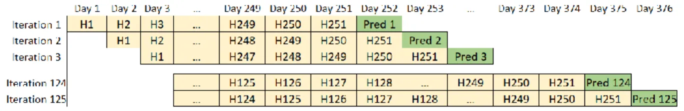
out-of-sample observations as the test set. To avoid the spreading of error after a long period, we make one-step-ahead predictions with sliding windows (Ntungo and Boyd, 1998). A historical sequence of the first 251 observations is used to forecast the value of day 252. For subsequent predictions, the head observation of the prior historical sequence is removed and a new observation is added at the tail of the sequence as depicted in Figure 1. For example, in the second iteration, the observation on day 252 is included and the observation of the first day is removed when predicting the risk factor on day 253. Thus, a total of 125 factor estimation sets with a size of 251 observations in each set are generated. The process is applied to all five factors individually.
For the LSTM model, the data is first transformed into sequences which are able to be fed into the network. One sequence is comprised of two parts, raw training data which is a certain length of continuous historical data and raw target data which is the prediction target of the corresponding training data. More formally, let 𝑥𝑖 denote the training data vector for sequence 𝑖, and 𝑦𝑖 denote the target data of the sequence 𝑖. I opt for an 𝑥 length of 100 observations and 𝑦 is the one-day-ahead data.7 For example, 𝑥
1 is a vector with observations from 𝑑𝑎𝑦1 to 𝑑𝑎𝑦100, thus 𝑦1 is the
observation on 𝑑𝑎𝑦101 which is the forecasted target of 𝑥1. I generate overlapping sequences for the whole dataset, thus sequence 𝑖 consist of observations from 𝑑𝑎𝑦𝑖 to 𝑑𝑎𝑦𝑖+99 as 𝑥𝑖 and the
observation of 𝑑𝑎𝑦𝑖+100 as 𝑦𝑖 as depicted in Figure 2.
Then the transformed sequences are split into two parts which are the in-sample set that is the training database used to train a neural network into a “predictor” and the out-of-sample set that is called the test set. The out-of-sample set consists of 125 sequences which are in line with the ARIMA model’s test set. The in-sample set is separated into a training set and a validation set with
6 As a robustness check, the predictions of risk factors using 100 historical observations are conducted.
Diebold-Mariano tests on the predictions made from 251 observations (ARIMA-251) and 100 observations (ARIMA-100) shows that, for the HML factor, the MSE of the ARIMA-251 predictions is significantly lower than the ARIMA-100 predictions by 0.094, while for the other factors, MSEs of the ARIMA-251 predictions are insignificantly (at 5% level) lower than the ARIMA-100 predictions.
7 The sequence of 100 observations is selected by trials. The sequence of 20, 30, 50, 80, 100, 150, 200, 300, 500 and
1000 observations were tested in the first round. Fischer and Krauss (2018) chose the sequence of 240 observations which is approximately one trading year. Thus the sequence of 240 and 250 observations were tested in the second round. Finally, the sequence of 100 observations is selected as it generates the lowest loss.
12
a split ratio that varies from 1:1 to 4:18. The split ratio is manually searched by observing the
smallest training error and the validation loss graphs in the following training steps.
4.1.2 Software and Libraries
The realizations from the LSTM and ARIMA models are conducted using Python 3.6 and a combination of its libraries. Pandas (McKinney, 2010) and Numpy (Van Der Walt et al., 2011) are used mainly for data preparation. The Statsmodels package is used for the ARIMA model forecasting. The main library for the LSTM network estimation is Keras (Gulli, 2017) with backend running Google TensorFlow. Also, several other packages are used to generate results graphs and figures, including Matplotlib and Seaborn.
4. 2 Methodology
To predict the returns of S&P 100 stocks, we use three models: a static LSTM network model, a hybrid ARIMA and Fama-French five factor model (ARIMA-FF) and a hybrid LSTM network and Fama-French five factor model (LSTM-FF). Our methodology consists of two main steps. At the first stage, returns of the 99 stocks are predicted using each of the three models. The ARIMA-FF model and the LSTM-ARIMA-FF model are known to have better practicability than the static LSTM model, thus we assume that all the sample stocks can be predicted using the two hybrid models, and only a portion of stocks will be trained by the static LSTM model. In the second step, pairwise comparisons are carried out among the three models. The comparisons between the static LSTM and the two hybrid models are confined to the sample of stocks that are successfully trained using the static LSTM. Additionally, the predictions of the whole stock set are involved in the comparison between the ARIMA-FF model and LSTM-FF model.
4.2.1 The Sole Static LSTM Model
As previously explained, neural network models need fine adjustments based on specific data sets. Thus, an LSTM model’s learning proficiency will be greatly reduced if the structure and
8 There is no rule of thumb for deciding on the split ratio between the training and validation sets. Usually the split is
tuned by trials starting from a given ratio. Granger (1993) suggests holding back 20 percent of the training database as a validation set. And Larsen et al. (1996) propose to start with a balanced split of 50 percent for both the training and validation sets considering the learning objective, scheme and curve.
13
parameters remain unchanged when it is applied on different data sets. Therefore, the static LSTM model is designed as a general structure that will exhibit failure or inefficient training on some of the 99 stocks using the criteria subsequently discussed.
The static LSTM model used herein has 4 layers: one input layer, two hidden layers and one output layer. There are no strict rules to frame an optimal neural network but some cautions need to be considered in the modeling process. A basic three-layer (one input layer, one hidden layer, and one output layer) neural network can be advanced to conduct deeper learning by adding hidden layers into it. With deeper structures, the neural network can perform better by capturing more statistical regularities (Hinton, 2006). However, the computational cost is very expensive when it comes to training a very deep network. Despite the computational cost, most of the problems can be solved using a one-hidden-layer network (Heaton, 2008). Thus, this thesis adopts two hidden layers where only one LSTM layer is structured and the other (a dense layer) is used as a transition to the output layer. The specific structure is as follows:
1) The input data are separated into a training set and a validation set with a ratio of 2:1. 2) The input layer has 100 nodes, receiving transformed return sequences.
3) The first hidden layer is the LSTM layer which is the key structure of the model. Following Boger and Guterman (1997) who conclude that the suitable number of neurons in the hidden layer is around 2/3 of the size of the input layers, the LSTM hidden layer is designed with 64 neurons. Since the time sequence cannot be shuffled, the dropout ratio and recurrent dropout ratio are set to zero. The learning rate is 0.019.
4) The second hidden layer is a dense10 layer that contains 32 nodes, used as a connection
layer between the LSTM layer and output layer to prevent overfitting caused by large node size gaps during the training process.
5) The output layer is a dense layer that has only one node which is consistent with the one-day prediction target.
6) The activation function, which is the converter in the neural network that transforms the given inputs into outputs, plays a very important role in realizing the non-linear properties
9 0.01 is a typical default value of initial learning rate (Bengio, 2012).
10 A dense layer is a fully connected layer that every node in the prior (preceding) layer is densely connected to the
dense layer neurons (keras. io, 2015). A fully connected layer can capture all combinations of features but is very computationally expensive.
14
of neural networks. The exponential linear unit (ELU) (Clevert, 2015) is chosen as the activation function in the two hidden layers. The special feature of the ELU function is its ability to fully identify and take the input values when the inputs are positive, while exponentially shrinking down the negative inputs. This feature enables the high calculation efficiency as well as the capability to deal with the gradient vanishing problem.
7) To prevent overfitting and to increase training efficiency, a callback of EarlyStopping11 is
added in the training process. The EarlyStopping has come to be used as a monitor for the training process. Once the validation loss is no longer decreasing by over 1 bps for more than 20 iterations12, the training process halts itself.
Using the above model, 99 stocks are trained and training failures are identified if any of the following conditions are met: (1) If the training process stops because of the gradient exploding problem; (2) If the estimated returns are unchangeable during the full time period, the model fails the training on that stock; (3) If the signs of the estimated returns are unchangeable (all positive or all negative), the training is seen as failure; and (4) If the range of estimated returns is smaller than 5% of the range of real returns, the stock is also considered as failed training. This step is used to categorize stocks into two sets: the static LSTM trained set which includes stocks only successfully trained by the static LSTM model and the full stock set containing all 99 stocks.
4.2.2 Hybrid LSTM and Fama-French Five Factor Model
The second model is a hybrid model with two prediction cores: the LSTM part as the main forecasting tool and the Fama-French five factor model as the proxy to account for the systematic risks captured in stock returns. The main difference between the above two vehicles in terms of their prediction ability is associated with a difference in the underlying methodology, where the LSTM tries to find the relationship between inputs and outputs based on historical information, while the Fama-French model uses its explanatory power for predicting stock returns by breaking down returns into financial factors. Considering the fact that the neural network calculation process
11 Earlystopping is a callback used to monitor the training process in order to end the training once the specific
performance measures are triggered. The loss and accuracy of validation datasets are usually used as the target for monitoring. Adopting the EarlyStopping is an efficient way to considerably prevent model overfitting (Bengio, 2012).
12 The number of training iterations is done by setting the patience argument. The exact patience numbers vary among
models and datasets. By reviewing performance plots, it can be analyzed how noisy the optimization process is, thereby the patience can be fine tuned. In this static LSTM model, settings are designed to be constant among different stocks data, thus the patience is arbitrarily selected as 20.
15
is often regarded as a “black box”, the disadvantage of applying the LSTM model is the difficulty of interpreting the predictions (Horel et al., 2018), whereas the hybridization can benefit from the financial implications of the Fama-French model.
In the first step, LSTM models are built for each risk factor to make predictions using historical data. The design of the LSTM model is similar to the sole LSTM model:
1) The split ratios of the input data for different risk factors are initialized to be around 4:113.
2) The model has the same four-layer structure as the static LSTM model with one 100-neuron input layer, one LSTM hidden layer, one dense hidden layer and a single neuron output layer.
3) ELU is the activation function for all models’ hidden layers.
4) EarlyStopping callbacks are added to monitor the training process. The monitored parameter of validation loss and the changing level of 1 bps are the same for all five factors, but the number of iterations (patience) before training stops differs based on the training properties of factors as certain factors’ trainings are easier to trigger the gradient explosion problem or overfitting.
As mentioned in the data preparation phase, predictions of 125 days (𝑡1-𝑡125) are produced by the LSTM models for each risk factor. Next, the predicted risk factors are fed into the Fama-French model to compute the predictions of stock returns. The betas of the risk factors for a stock are generated by regressing its returns in 2017 (251 trading days) on the cotemporaneous real risk factors. The estimated betas and intercepts are then used to forecast the returns of 𝑡1 to 𝑡125 with the factor values estimated by the LSTM models. The above procedures are repeated for all 99 stocks and all the predictions are kept for the further comparisons.
13 The split ratio varies when it comes to different datasets. The specific ratio that is applied for each factor is chosen
by trials, where the selected rate is the one causes the lowest training error. The static LSTM model adopts an arbitrary ratio of 2:1 as the design of static model is aiming to show that the LSTM networks are limited when the model adjustments are restricted as applied to different data sets.
16 4.2.3 Hybrid ARIMA and Fama-French Five Factor Model
The ARIMA-FF model takes advantage of the ARIMA model’s prediction power using time series data and the explanatory power of the Fama-French model to make stock return predictions. To build the ARIMA model, the following pre-tests are needed:
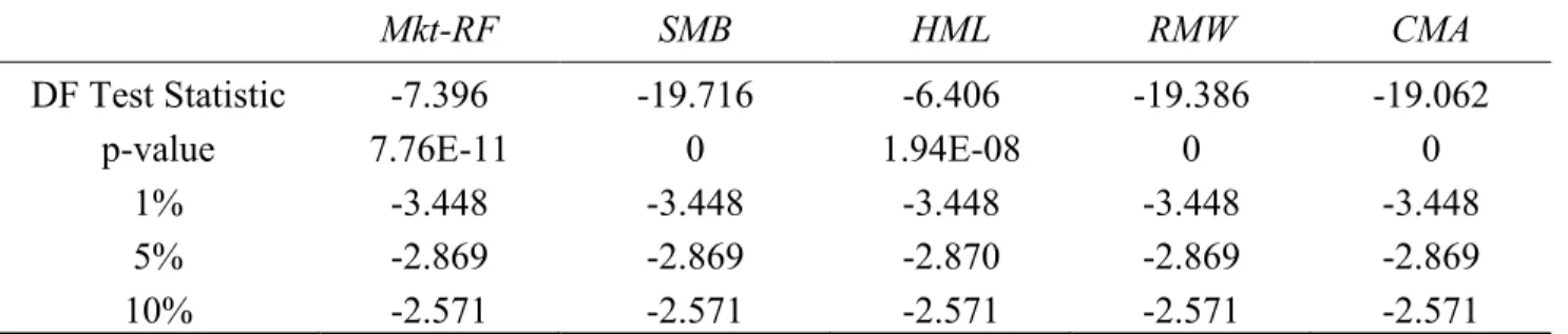
1) As previously mentioned, ARIMA models require the time series to be stationary for them to be effective. The Augmented Dickey-Fuller (ADF) test is used to test unit roots in the time series, where the null hypothesis is that the time series is non-stationary. In this thesis, ADF tests are implemented by Adfuller tests from Python’s Statsmodel library. Table 1 shows the ADF test results where all the test statistics are significant at the 1% level, indicating that the five FF factors are stationary. Thus, the differencing parameters (d) are set to 0 in all risk factor ARIMA models.
2) To decide the units of the time lags (p) and residuals (q), ACF and PACF plots in addition to BIC values are used, and are also validated by examining model residual distributions using Python’s Statsmodel library.
Consistent with the LSTM model, predictions for risk factors are also made as one-day ahead for 125 days (𝑡1-𝑡125). The process of combining the ARIMA model with the Fama-French model is same as that for the LSTM-FF model. The same betas and ARIMA estimated risk factors are used in generating the predictions of all 99 stocks.
I employ two measures in order to compare the prediction accuracy of the models: Mean Squared Error (MSE) and moving direction index (D). The MSE generates the statistical results of the models’ predictions, while the moving direction index provides a more intuitive comparison of the models. The MSE is defined as:
𝑀𝑆𝐸𝑖 = 1
𝑁∑(𝑦𝑖,𝑡− 𝑦̂𝑖,𝑡
𝑁
𝑡=1
)2 , (3)
where N equals 125, denoting the total number of observations of stock 𝑖 and 𝑦𝑖,𝑗 and 𝑦̂𝑖,𝑗 are the
historical data and estimated data of stock 𝑖 at time 𝑡 respectively.
Let 𝑑𝑖,𝑡 denote the moving direction index for stock 𝑖 at time 𝑡, which takes on the value of one if the sign of the estimated return is the same as that of the real return, and zero otherwise.. Thus 𝐷𝑖
17
presents the ratio of estimates with correctly identified moving directions. The prediction is of value only when the ratio is above 50% (Kryzanowski et al., 1993).
𝐷𝑖 = 1
𝑁∑ 𝑑𝑖,𝑡
𝑁
𝑡=1
(4) Therefore, for each stock 𝑖, the LSTM-FF and ARIMA-FF models produce MSEs and price moving directions for the 99 stocks and the static LSTM model generates the two measures for the successfully trained stocks.
Difference in means tests are carried out to examine whether a model statistically outperforms the others in terms of the return predictions for the selected stocks.
5. Results
5.1 Fama-French Risk Factors Predictions
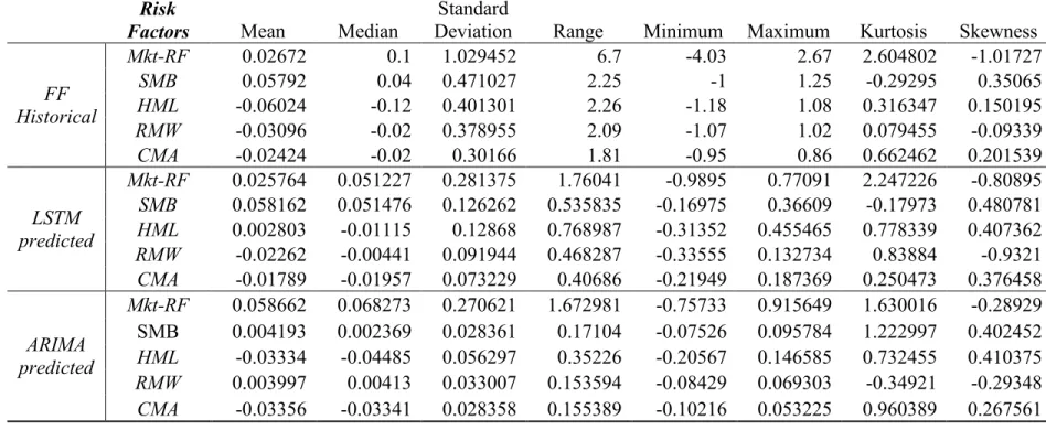
In the first stage of the model building process, the Fama-French risk factors are predicted by the LSTM and ARIMA models. Table 2 describes the summary statistics of the raw risk factors and the LSTM and ARIMA predicted risk factors. Compared to the ARIMA predicted results, the means of the LSTM predicted risk factors are closer to those of the raw factors with a MSE of 0.00082 which is lower than the 0.00119 obtained from the ARIMA predictions.
One of the biggest concerns in forecasting is that both the LSTM and the ARIMA predicted factors fail to reach as broad ranges as the actual raw data. It is likely that the factor predictions of the ARIMA models are not realistically volatile. To demonstrate this problem, we compute the estimation range broadness as a ratio of the estimated range of a factor over its raw range. As reported in Table 2, the LSTM predicted HML has the largest range percentage at a very modest 34%, while the smallest range comes from the ARIMA predicted RMW with a meager percentage of 7.3%. The estimation ranges for all the risk factors in the LSTM model are above 20%, while the Mkt-RF prediction range of 25% for the ARIMA model is the only one above 20%. Figure 3 plots the time-series of the estimated risk factors and raw data which visually shows that the LSTM estimates have broader ranges than the ARIMA predictions. The variations of the ARIMA model predictions are insignificant and with very narrow ranges for SMB and RMW. This result could
18
be caused by two possible reasons. First, the selected ARIMA model might not be very suitable for the SMB and RMW factors. Second, the data length might not be adequate for efficient model training.14
5.2 Stock Return Prediction and Comparison
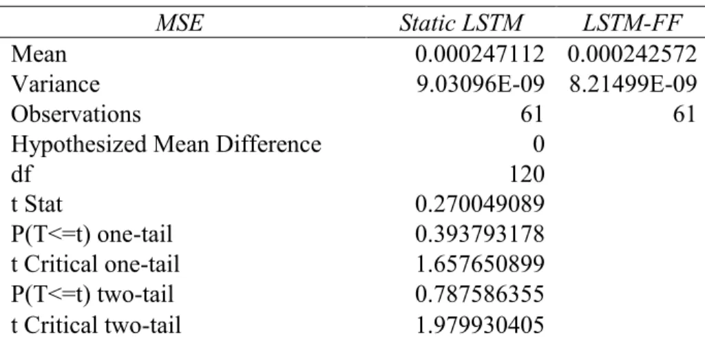
We are able to test 99 of the 101 S&P 100 stocks using our three models. Table 3 shows the training success and each model’s fit rate, defined as the ratio of the number of successfully trained stocks over the total number of stocks in the sample. While two hybrid models are able to fit the full sample set, the static LSTM model only fits 62% of the sample (61 out of 99 stocks) demonstrating at least the broad applicability of the hybrid models if not helping to establish their superior accuracy. These results are consistent with the hypothesis 3.1 which argues that the LSTM model has a poorer prediction capacity when the model is restricted from structural adjustments.
Table 4 presents the summary performance of the models’ predictions for a subset consisting of the stocks that were successfully trained by the static LSTM model and the full stock sample of 99 stocks. As previously defined, 𝐷𝑖 is the moving direction ratio of stock 𝑖. 45.9% (28 out of 61) of stocks predictions produced by the static LSTM model are seen as valuable with the criteria of a 𝐷𝑖 above 50%. In contrast, within the static LSTM trained set (61 stocks), 44 (72.1%) and 34 (55.7%) stock predictions outperform the random selected probability generated by the LTSM-FF and the ARIMA-FF models respectively. These rates drop to 62.6% for the LSTM-FF model and 52.5% for the ARIMA-FF model when applied to the full stock set. In other words, the LSTM-FF model generates more effective predictions than the remaining two models, with the poorest performing model being the static LSTM model.
5.2.1 The Static LSTM vs. The Hybrid Models
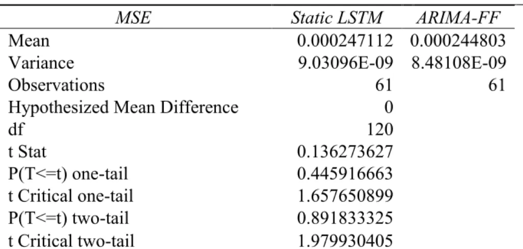
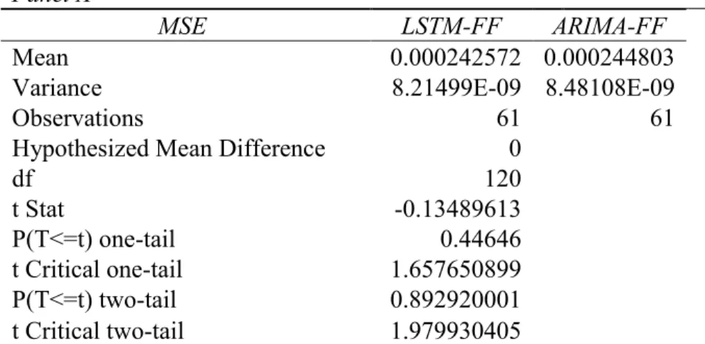
Panel A of Table 5.1 presents the results of the difference in means tests for the static LSTM and LSTM-FF predictions using 61 stocks. The mean MSE for the static LSTM is 1.9% higher than that of the LSTM-FF model. However, this difference is not statistically significant. In contrast,
14 A robust test is conducted using a full period data set (from the year of 1963). The predictions using the full period
data slightly outperformed any shorter periods in terms of MSE and prediction result ranges. However, most of the studies adopt a relatively short horizon. (Particularly, some studies on idiosyncratic risk use data for long periods) This could be pursued in further investigation.
19
the mean of the directional indicator 𝐷𝑖 for the LSTM-FF predictions reported in Panel B of Table
5.1 is significantly higher than that of the static LSTM predictions by 4.6%.
We find similar results for the comparison between the static LSTM and ARIMA-FF predictions reported in Table 5.2. The means of the MSEs between two models are slightly different and fail to provide evidence for the conjecture that the hybrid model generates lesser prediction errors. Not surprisingly, the mean of the ARIMA-FF 𝐷𝑖 is significantly higher than the mean of static LSTM 𝐷𝑖 by 3.1%.
5.2.2 LSTM-FF vs. ARIMA-FF
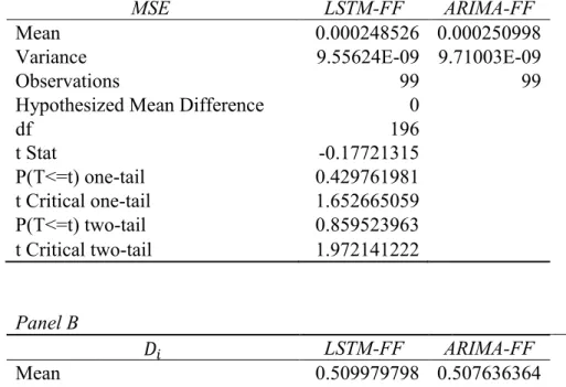
The comparison of the two hybrid models is conducted using both the static trained set and the full stock set. Based on the results reported in Panel A of Tables 5.3 and 5.4, there is no statistically significant difference in the mean MSEs of the LSTM-FF model and the ARIMA-FF model for both data sets. Contrary to the results reported in Section 5.2.1, Panel B of Tables 5.3 and Table 5.4 reveal there is no statistically significant change in the mean differences in the moving directions of both models. Therefore, these results do not support the hypothesis 3.3 which argues that the LSTM hybrid model is a better predictor of stock returns than the ARIMA hybrid model.
6. Limitations
Although some slight differences are found between the static LSTM model and the hybrid models, we fail to find strong support of the main research question of the difference in forecasting ability between the neural network hybrid model and the ARIMA hybrid model. There are some aspects that might lead to the limitations of the methodology of this thesis. Namely, selecting the S&P100 stocks as the sample might confine the research’s generalizability due to the small number of stocks in the bucket and the bias of the company size. The reason for not adopting a larger and more diversified stock sample set is the constraints of computing ability and the relatively lengthy training process.
As shown in the results, both the LSTM-FF model and the ARIMA-FF model generate better predictions on the static LSTM trained set than on the full stock set. The causes have not been investigated in this thesis and could be examined in future studies. Knowing the reasons why the
20
models show varied fitness on different stocks, it is possible to test the predictability with certain conditions and to construct corresponding investment strategies.
Another limitation is the data horizon of the ARIMA model. In this thesis, I take one-year length of historical Fama-French factors data to make one-ahead predictions. However, it is found that using the full length of historical data to make the out-of-sample forecasting gives the best output of FF risk factors. The tuning of the ARIMA model is beyond the research goal of this thesis, but can be deployed as a further test.
7. Conclusion
Neural networks are widely applied to forecasting in various fields. The introduction of LSTM networks enlightens time series’ predictions due to their superior algorithm as well as their high adaptability. However, being difficult to fit finance intuition has limited their acceptance to the finance and economics. This situation encourages us to utilize LSTM networks in an interpretable way where we come up with the return forecasting LSTM-FF hybrid model, taking advantage of both LSTM networks’ time series forecasting intelligence and the Fama-French model’s explanatory ability. A static LSTM model and an ARIMA-FF model are designed in order to compare the LSTM-FF prediction accuracy with that of normal LSTM networks and traditional frequentist models.
The benefit of using hybrid models is that they have broader applicability since not every stock needs to have a complete time series of returns. Usually, neural networks provide good predictions but they are time-consuming due to the need for them to be trained on every individual stock. Additionally, in the case of newly introduced securities such as carve-outs or IPOs15, a neural net
cannot be applied. The use of a static LSTM network reveals that not changing the network’s structure or hyper-parameters will reduce its goodness of fit and restrict its predictability. The results reveal that amongst 99 S&P100 stocks, 61 can be predicted by the same structured LSTM network, while hybrid models can be applied to all stocks. Also, in terms of their prediction accuracy, two hybrid models significantly outperform the static LSTM model when focusing on the price movement direction. However, the comparison of the LSTM-FF and the ARIMA-FF
21
models reveals no statistically significant difference between their predictions. Our findings fail to support the assumption that the LSTM-FF models are able to generate better predictions than the ARIMA-FF models.
Further investigation into this topic could be addressed by the work of future researchers. One of the possible improvements of this study is embedded in the LSTM network’s design. Given the adjustability and flexibility of LSTM networks, several modifications to the networks’ structure and hyper-parameters could be made. On the other hand, increasing the model’s complexity or tuning the model’s settings might result in better prediction accuracy.
22 References
Ang, A., Bekaert, G., & Wei, M. (2008). The term structure of real rates and expected inflation. The Journal of Finance, 63(2), 797-849.
Ang, A., Bekaert, G., & Wei, M. (2007). Do macro variables, asset markets, or surveys forecast inflation better?. Journal of monetary Economics, 54(4), 1163-1212.
Babu, C. N., & Reddy, B. E. (2014). A moving-average filter based hybrid ARIMA-ANN model for forecasting time series data. Applied Soft Computing Journal, 23, 27–38.
Bengio, Y. (2009). Learning deep architectures for AI. Foundations and trends® in Machine Learning, 2(1), 1-127.
Bengio, Y. (2012). Practical recommendations for gradient-based training of deep architectures. In Neural networks: Tricks of the trade (pp. 437-478). Springer, Berlin, Heidelberg.
Bergstra, J., & Bengio, Y. (2012). Random search for hyper-parameter optimization. Journal of Machine Learning Research, 13(Feb), 281-305.
Bianchi, L., Jarrett, J., & Hanumara, R. C. (1998). Improving forecasting for telemarketing centers by ARIMA modeling with intervention. International Journal of Forecasting, 14(4), 497-504. Boger, Z., & Guterman, H. (1997, October). Knowledge extraction from artificial neural network
models. In 1997 IEEE International Conference on Systems, Man, and Cybernetics. Computational Cybernetics and Simulation (Vol. 4, pp. 3030-3035). IEEE.
Brennan, M. J., Chordia, T., & Subrahmanyam, A. (1998). Alternative factor specifications, security characteristics, and the cross-section of expected stock returns. Journal of Financial Economics, 49(3), 345–373.
Campbell, J. Y. (1987). Stock returns and the term structure. Journal of financial economics, 18(2), 373-399.
Campbell, J. Y., & Thompson, S. B. (2007). Predicting excess stock returns out of sample: Can anything beat the historical average?. The Review of Financial Studies, 21(4), 1509-1531. Campbell, J. Y., & Yogo, M. (2006). Efficient tests of stock return predictability. Journal of
23 financial economics, 81(1), 27-60.
Cao, Q., Leggio, K. B., & Schniederjans, M. J. (2005). A comparison between Fama and French’s model and artificial neural networks in predicting the Chinese stock market. Computers and Operations Research, 32(10), 2499–2512.
Clevert, D. A., Unterthiner, T., & Hochreiter, S. (2015). Fast and accurate deep network learning by exponential linear units (ELUs). arXiv preprint arXiv:1511.07289.
Cochrane, J. H. (2005). Time series for macroeconomics and finance. Manuscript, University of Chicago, 1-136.
Enders, W. (1988). ARIMA and cointegration tests of PPP under fixed and flexible exchange rate regimes. The Review of Economics and Statistics, 504-508.
Fama, E. F., & French, K. R. (1988). Permanent and temporary components of stock prices. Journal of political Economy, 96(2), 246-273.
Fama, E. F., & French, K. R. (1992). The cross‐section of expected stock returns. the Journal of Finance, 47(2), 427-465.
Fama, E. F., & French, K. R. (2015). A five-factor asset pricing model. Journal of financial economics, 116(1), 1-22.
Fama, E. F., & French, K. R. (2018). Choosing factors. Journal of Financial Economics, 128(2), 234-252.
Fischer, T., & Krauss, C. (2018). Deep learning with long short-term memory networks for financial market predictions. European Journal of Operational Research, 270(2), 654-669. François, C. (2015). Keras. Keras. io.
Gers, F. A., Schmidhuber, J., & Cummins, F. (2000). Learning to forget: Continual prediction with LSTM. Neural Computation, 40,2451-2471.
Guresen, E., Kayakutlu, G., & Daim, T. U. (2011). Using artificial neural network models in stock market index prediction. Expert Systems with Applications, 38(8), 10389–10397.
24 Catalogue. Oxford University Press, Oxford, 1993.
Greff, K., Srivastava, R. K., Koutník, J., Steunebrink, B. R., & Schmidhuber, J. (2016). LSTM: A search space odyssey. IEEE transactions on neural networks and learning systems, 28(10), 2222-2232.
Gulli, A., & Pal, S. (2017). Deep Learning with Keras. Packt Publishing Ltd.
Hadavandi, E., Shavandi, H., & Ghanbari, A. (2010). Integration of genetic fuzzy systems and artificial neural networks for stock price forecasting. Knowledge-Based Systems, 23(8), 800– 808.
Hansen, L. K., & Salamon, P. (1990). Neural network ensembles. IEEE Transactions on Pattern Analysis & Machine Intelligence, (10), 993-1001.
Hawley, D. D., Johnson, J. D., & Raina, D. (1990). Artificial Neural Systems: A New Tool for Financial Decision-Making. Financial Analysts Journal, 46(6), 63–72.
Heaton, J. (2008). The number of hidden layers. Heaton Research Inc.
Hinton, G. E. (2012). A practical guide to training restricted Boltzmann machines. In Neural networks: Tricks of the trade (pp. 599-619). Springer, Berlin, Heidelberg.
Hinton, G. E., Osindero, S., & Teh, Y. W. (2006). A fast learning algorithm for deep belief nets. Neural computation, 18(7), 1527-1554.
Hochreiter, S., Bengio, Y., Frasconi, P., & Schmidhuber, J. (2001). Gradient flow in recurrent nets: the difficulty of learning long-term dependencies. A field guide to dynamical recurrent neural networks, IEEE Press, 2001.
Hochreiter, S., & Schmidhuber, J. (1997). Long short-term memory. Neural computation, 9(8), 1735-1780.
Horel, E., Mison, V., Xiong, T., Giesecke, K., & Mangu, L. (2018). Sensitivity based Neural Networks Explanations. arXiv preprint arXiv:1812.01029.
Hou, K., Xue, C., & Zhang, L. (2015). Digesting anomalies: An investment approach. The Review of Financial Studies, 28(3), 650-705.
25
Hou, K., Mo, H., Xue, C., & Zhang, L. (2018). Which factors?. Review of Finance, 23(1), 1-35. Kaastra, I., & Boyd, M. S. (1995). Forecasting futures trading volume using neural networks.
Journal of Futures Markets, 15(8), 953-970.
Kaastra, I., & Boyd, M. (1996). Designing a neural network for forecasting financial and economic time series. Neurocomputing, 10(3), 215–236.
Khashei, M., & Bijari, M. (2010). An artificial neural network (p, d, q) model for timeseries forecasting. Expert Systems with Applications, 37(1), 479–489.
Kuremoto, T., Kimura, S., Kobayashi, K., & Obayashi, M. (2014). Time series forecasting using a deep belief network with restricted Boltzmann machines. Neurocomputing, 137, 47–56. Krogh, A., & Vedelsby, J. (1995). Neural network ensembles, cross validation, and active learning.
In Advances in neural information processing systems, pp. 231-238.
Kryzanowski, L., Galler, M., & Wright, D. W. (1993). Using artificial neural networks to pick stocks. Financial Analysts Journal, 49(4), 21-27.
Längkvist, M., Karlsson, L., & Loutfi, A. (2014). A review of unsupervised feature learning and deep learning for time-series modeling. Pattern Recognition Letters, 42(1), 11–24.
Larsen, J., Hansen, L. K., Svarer, C., & Ohlsson, M. (1996, September). Design and regularization of neural networks: the optimal use of a validation set. In Neural Networks for Signal Processing VI. Proceedings of the 1996 IEEE Signal Processing Society Workshop (pp. 62-71). IEEE.
Leung, M. T., Daouk, H., & Chen, A.-S. (2000). Forecasting stock indices: a comparison of classification and level estimation models. International Journal of Forecasting, 16(2), 173– McKinney, W. (2010, June). Data structures for statistical computing in python. In Proceedings
of the 9th Python in Science Conference, vol. 445, pp. 51-56.
McLean, R. D., & Pontiff, J. (2016). Does academic research destroy stock return predictability?. The Journal of Finance, 71(1), 5-32.
Moskowitz, T. J., Ooi, Y. H., & Pedersen, L. H. (2012). Time series momentum. Journal of financial economics, 104(2), 228-250.
26
Nelson, D. M. Q., Pereira, A. C. M., & De Oliveira, R. A. (2017). Stock market’s price movement prediction with LSTM neural networks. Proceedings of the International Joint Conference on Neural Networks, 2017-May(Dcc), 1419–1426.
Newton, D. Are all forecasts made equal? Conditioning models on fit to improve accuracy. Review of Pacific Basin Financial Markets and Policies, forthcoming.
Novy-Marx, R. (2013). The other side of value: The gross profitability premium. Journal of Financial Economics, 108(1), 1-28.
Ntungo, C., & Boyd, M. (1998). Commodity futures trading performance using neural network models versus ARIMA models. Journal of Futures Markets: Futures, Options, and Other Derivative Products, 18(8), 965-983.
Odom, M. D., & Sharda, R. (1990, June). A neural network model for bankruptcy prediction. In 1990 IJCNN International Joint Conference on neural networks (pp. 163-168). IEEE. Poterba, J. M., & Summers, L. H. (1988). Mean reversion in stock prices: Evidence and
implications. Journal of financial economics, 22(1), 27-59.
Rather, A. M., Agarwal, A., & Sastry, V. N. (2015). Recurrent neural network and a hybrid model for prediction of stock returns. Expert Systems with Applications, 42(6), 3234–3241.
Roll, R. (1977). A critique of the asset pricing theory's tests Part I: On past and potential testability of the theory. Journal of financial economics, 4(2), 129-176.
Rumelhart, D. E., Hinton, G. E., & Williams, R. J. (1986). Learning representations by back-propagating errors. Nature, 323 (6088): 533–536.
Sharpe, W. F. (1964). Capital asset prices: A theory of market equilibrium under conditions of risk. The journal of finance, 19(3), 425-442.
Thomakos, D. D., & Guerard Jr, J. B. (2004). Naı̈ve, ARIMA, nonparametric, transfer function and VAR models: A comparison of forecasting performance. International Journal of Forecasting, 20(1), 53-67.
Titman, S., Wei, K. J., & Xie, F. (2004). Capital investments and stock returns. Journal of financial and Quantitative Analysis, 39(4), 677-700.
27
Van Der Walt, S., Colbert, S. C., & Varoquaux, G. (2011). The NumPy array: a structure for efficient numerical computation. Computing in Science & Engineering, 13(2), 22.
Vougas, D. V. (2004). Analysing long memory and volatility of returns in the Athens stock exchange. Applied Financial Economics, 14(6), 457-460.
Walczak, S. (2001). An Empirical Analysis of Data Requirements for Financial Forecasting with Neural Networks. Journal of Management Information Systems, 17(4), 203–222.
Wang, J. Z., Wang, J. J., Zhang, Z. G., & Guo, S. P. (2011). Forecasting stock indices with back propagation neural network. Expert Systems with Applications, 38(11), 14346–14355. Welch, I., & Goyal, A. (2007). A comprehensive look at the empirical performance of equity
premium prediction. The Review of Financial Studies, 21(4), 1455-1508.
Werbos, P. J. (1975). Beyond Regression: New Tools for Prediction and Analysis in the Behavioral Sciences. Harvard University.
Werbos, P. J. (1982). Applications of advances in nonlinear sensitivity analysis. In System modeling and optimization (pp. 762-770). Springer, Berlin, Heidelberg.
Zhang, G., Patuwo, B. E., & Hu, M. Y. (1998). Forecasting with artificial neural networks: The state of the art. International journal of forecasting, 14(1), 35-62.
Zhang, P. G. (2003). Time series forecasting using a hybrid ARIMA and neural network model. Neurocomputing, 50, 159–175.
28 Figures
Figure 1. ARIMA Model Data Sequences Structure
H1 to H251 indicate the 251 historical risk factor observations in an iteration and the prediction is made on the following day after H251. Pred1 to Pred125 are the out-of-sample predicted factors generated in 125 iterations.
Figure 2. LSTM networks Data Sequences Structure
LSTM networks ask for input data as sequences which are combined by X as the training vectors and Y as the targets. All sequences are of the same length containing 101 days of historical values. Y is the one-day-ahead observation of corresponding X.
29
Figure 3. Fama-French Risk Factors – Historical Values and Predictions
-4 -2 0 2 Mk t-RF -1.2 -0.2 0.8 SMB -1.3 -0.3 0.7 H ML -1.2 -0.2 0.8 RMW -1.1 -0.1 0.9 CMA