Spectral
–
spatial feature learning for
hyperspectral imagery classification
using deep stacked sparse
autoencoder
Ghasem Abdi
Farhad Samadzadegan
Peter Reinartz
Ghasem Abdi, Farhad Samadzadegan, Peter Reinartz,“Spectral–spatial feature learning for hyperspectral imagery classification using deep stacked sparse autoencoder,”J. Appl. Remote Sens.11(4),
hyperspectral imagery classification
using deep stacked sparse autoencoder
Ghasem Abdi,
a,*
Farhad Samadzadegan,
aand Peter Reinartz
baUniversity of Tehran, College of Engineering, Faculty of Surveying and Geospatial
Engineering, Tehran, Iran
bGerman Aerospace Centre (DLR), Remote Sensing Technology Institute,
Department of Photogrammetry and Image Analysis, Weßling, Germany
Abstract. Classification of hyperspectral remote sensing imagery is one of the most popular topics because of its intrinsic potential to gather spectral signatures of materials and provides distinct abilities to object detection and recognition. In the last decade, an enormous number of methods were suggested to classify hyperspectral remote sensing data using spectral features, though some are not using all information and lead to poor classification accuracy; on the other hand, the exploration of deep features is recently considered a lot and has turned into a research hot spot in the geoscience and remote sensing research community to enhance classification accuracy. A deep learning architecture is proposed to classify hyperspectral remote sensing imagery by joint utilization of spectral–spatial information. A stacked sparse autoencoder pro-vides unsupervised feature learning to extract high-level feature representations of joint spectral– spatial information; then, a soft classifier is employed to train high-level features and to fine-tune the deep learning architecture. Comparative experiments are performed on two widely used hyperspectral remote sensing data (Salinas and PaviaU) and a coarse resolution hyperspectral data in the long-wave infrared range. The obtained results indicate the superiority of the pro-posed spectral–spatial deep learning architecture against the conventional classification methods. ©2017 Society of Photo-Optical Instrumentation Engineers (SPIE)[DOI:10.1117/1.JRS.11.042604] Keywords:deep features; deep learning; hyperspectral imagery classification; softmax regres-sion; spectral–spatial unsupervised feature learning; stacked sparse autoencoder.
Paper 170368SS received May 1, 2017; accepted for publication Jul. 26, 2017; published online Aug. 22, 2017.
1 Introduction
With the recent technological advances in remote sensing systems and the accessibility of hyper-spectral data, the geoscience and remote sensing research community is increasing utilization of well-defined spectral information of hyperspectral images in a wide range of practical applications.1,2Hyperspectral image data are comprised of hundreds of continuous narrow spec-tral bands, resulting in high specspec-tral information for the identification of diverse physical mate-rials and leading thereby to enhanced image classification results.3,4In the last decade, a large number of methods have been widely investigated for addressing the ill-posed classification problems of hyperspectral remote sensing data by considering high dimensionality and complex-ity of spectral features.5–9In this context, two popular dimensionality reduction strategies are widely used to overcome the finite training set problem with high dimensionality of hyperspectral remote sensing data. The dimensionality reduction by transform uses a transformation function to compress data in some optimal sense, while the dimensionality reduction by band selection extracts a suitable band subset to indicate data through a definite optimum criterion.10
Further-more, joint utilization of spectral–spatial information of hyperspectral imagery has been
*Address all correspondence to: Ghasem Abdi, E-mail:[email protected] 1931-3195/2017/$25.00 © 2017 SPIE
extensively investigated to improve the classification accuracy by considering the spatial infor-mation represented by neighboring pixels mostly pertaining to one class.11–13 Most of the existing methodologies can determine shallow handcrafted features or transform-based filters of the original data, which are not robust enough to deal with hyperspectral imagery classifi-cation challenges.14The exploration of deep features has recently attracted much consideration and is now a research hot spot in the geoscience and remote sensing research community for improving classification results via an extremely powerful deep learning model.15–23
Recently, several deep learning architectures have prospered24and have been employed in
audio recognition,25 natural language processing,26 and many classification tasks.27,28 In this
context, deep learning researchers have expanded deep architectures as a replacement for the traditional shallow architectures motivated by the human brain architectural model.29 From the deep learning point of view, deep belief networks train one layer in an unsupervised way via restricted Boltzmann machines.30,31Autoencoder (AE) and its variants train the intermediate layers of representation in an unsupervised manner.32,33Unlike AEs, the sparse coding algo-rithms extract sparse representations of the original data by learning a dictionary.34 Mean-while, convolutional neural networks, the most representative supervised deep learning archi-tecture, allow the deep architecture to learn high-level feature descriptors and to convert the input space into representations that can clearly enhance the classification performance.35In this
con-text, a set of learnable filters is convolved across the input volume to form a stacked activation map of the filters, i.e., the network learns filters that activate when it detects some specific type of features at some spatial position in the input data. More detailed descriptions about the deep learning algorithms can be observed in the machine learning research literature.36,37
Deep learning-based classification involves making a deep architecture for the pixel-based data representation and classification by extracting more robust and abstract descriptors to enhance the classification results. Deep learning pixel-based classification of hyperspectral imagery contains data input, hierarchical deep learning model training, and classification steps. The input vector could be comprised of spectral, spatial, or joint utilization of spectral– spatial descriptors. Next, a deep architecture is designed to train the feature representations of the input data. The last step contains hard or soft classification using the learned features at the top layer of the deep learning model, the hard classifiers, such as support vector machines (SVMs), output an integer classification result. The soft classifiers, such as logistic regression, can optimize the pretrained model and estimate a probability distribution of the classification result.16,38,39Deep learning-based hyperspectral imagery classification is a new subject in the geoscience and remote sensing research community and limited research has been conducted in this field of study.
From the autoencoder-based deep learning point of view, Chen et al.16 proposed stacked autoencoder via traditional spectral, spatial, and a deep spectral–spatial learning model to obtain the best classification results by a hybrid framework of principle component analysis (PCA), deep learning architecture, and a softmax classifier to optimize the pretrained model and predict land cover classification results. Experiments and results conducted over two public, Kennedy Space Center (KSC) and Pavia, datasets proved that the proposed method provides statistically higher accuracy than the SVM classifier. In addition, the experimental results indicated that deeper features mostly lead to better classification performance. Tao et al.17proposed a stacked autoencoder using multiscale spectral–spatial features in a linear SVM to obtain the highest classification results. Experiments and results conducted over Pavia and PaviaU datasets indi-cated that the proposed method provides more discriminative features than the handcrafted spec-tral–spatial features. The experimental results illustrated that the learned spectral–spatial feature representation can be used for multiple images. Zhao et al.21 proposed a new spectral–spatial deep learning-based classification framework that combines spectral–spatial information using hyperspectral imagery of appropriate spatial resolution in a stacked sparse autoencoder to extract high-level feature representations, followed by a random forest classifier to provide better trade-off among performance, accuracy, and processing time compared to traditional classifiers. Experiments conducted on two commonly used hyperspectral datasets (Indian Pines and KSC) showed that the new feature improves the classification results compared with the original hyperspectral imagery. Furthermore, the proposed framework provides higher classification accuracy and stronger performance when compared with other classification techniques.
Wang et al.22presented a hybrid framework of PCA, guided filtering, and stacked autoencoder as an efficient deep learning architecture for hyperspectral data classification. Experiments con-ducted over two public, PaviaU and Salinas, datasets demonstrated that the proposed spec-tral–spatial hyperspectral image classification method provides better results when compared with some other commonly used methods. In the above papers, many ways were proposed to classify hyperspectral imagery by deep learning mechanisms; they provided fascinating inno-vations for classification and practical applications. Deep learning-based hyperspectral imagery classification remains quite challenging because of its novelty and limited research up to now. This paper presents a deep learning-based hyperspectral imagery classification technique and addresses the superiority of the proposed method against a large number of traditional classifiers.
2 Proposed Method
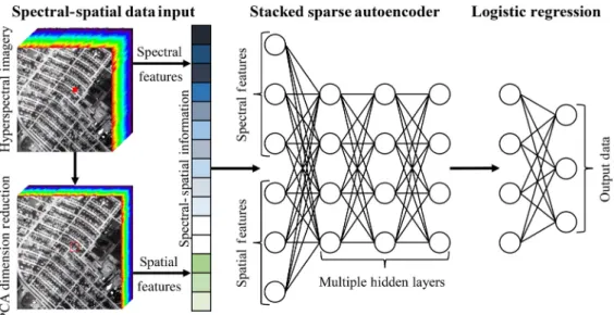
In this paper, we propose spectral–spatial feature learning for hyperspectral imagery classifica-tion using a deep stacked sparse autoencoder (DSSAE). In this context, a stacked sparse autoen-coder provides unsupervised feature learning to extract high-level feature representations of joint spectral–spatial information; then, a soft classifier is employed to train high-level features and to fine-tune the deep learning architecture. Figure1shows the general structure of the proposed method.
2.1
Spectral
–
Spatial Feature Extraction
The spectral–spatial feature descriptors are concatenated to construct the joint spectral–spatial classification framework. In this context, the raw spectral information is first considered (xspectral¼ fxk;1; xk;2; : : : ; xk;sg, where xspectral is the raw spectral data at the k’th pixel withs bands), because it consists of the most basic information from the classification point of view. Furthermore, the first several principle components (PCs) of a local window are considered as the spatial feature descriptors (xspatial¼ fxk;1; xk;2; : : : ; xk;d; : : : ; xk;sg, wherexspatial is the local
information at thek’th pixel with the firstdPC bands) to enhance the classification results; the obtained features are then stacked to make a hybrid set of joint spectral–spatial information.
2.2
Stacked Sparse Autoencoder
A shallow sparse autoencoder introduces a specific kind of neural network containing input, hidden, and reconstruction layers that can be employed to train the high-level feature represen-tations in an unsupervised manner.40,41 In other words, sparse autoencoder tries to estimate
a reconstruction function that maximizes the similarity score of decoding and input layer functions.21
In the training phase of an autoencoder, an encoder transfer function is applied to map an input vector into an abstract feature representation of the input vector as the hidden layer
EQ-TARGET;temp:intralink-;e001;116;687
z¼fðWzxþbzÞ; (1)
where Wz and bz indicate the weights and biases of the input to hidden layer, respectively.
Furthermore, the logistic sigmoid function,fðxÞ ¼ ½1þexpð−xÞ−1, is used to obtain nonlinear mapping of both the encoder and decoder transfer functions. Moreover, the hidden representa-tion is employed to reconstruct an approximarepresenta-tion of the input vector using a decoder transfer function from output layer
EQ-TARGET;temp:intralink-;e002;116;596
y¼fðWyzþbyÞ; (2)
whereWyandbyindicate the weights and biases of the hidden to output layer, respectively. In
general, the optimal parameters are estimated by minimizing the reconstruction error with spar-sity constraint and weight decay terms
EQ-TARGET;temp:intralink-;e003;116;529Jcos t¼ 1 M XM i¼1 1 2kyi−xik22 þλ2X l X i X j ðWði;jlÞÞ2þηX S j¼1 KLðrk¯rjÞ; (3)
where the first term denotes an average sum of squares error term that demonstrates the reconstruction error of M training samples,17 the second term indicates the weight decay term that is applied to reduce the over fitting of autoencoder via managing the weights amplitude (whereλis a weight decay parameter,Wði;jlÞdenotes the connection between thei’th unit in layer l−1and thej’th unit in layerl),42and the third term is a sparsity penalty term thatηcontrols the weight of the term andKLðrkr¯jÞillustrates a Kullback–Leibler divergence, a function used to
measure the difference between Bernoulli distributions of the expected activation over the train-ing set of hidden unitjand its target value, to be penalized by the sparsity constant to enforce the average latent unit activation to be close to the target value17
EQ-TARGET;temp:intralink-;e004;116;369KLðrkr¯ jÞ ¼ XS j¼1 rlog ¯r rj þ ð1−rÞlog 11−−¯r rj ; (4)
whereris the parameter of desired sparsity and¯rj¼M1 PM
i¼1½yjðxiÞdenotes the average
acti-vation of hidden unitjof the training dataxi. The minimumKLdistance is achieved byr¼r¯j
and extends up to infinity as r¯j increases, enforcing r¯j not to significantly deviate from the
desired sparsity valuer; the smaller desired sparsity value commonly leads to a sparser repre-sentation. Furthermore, the minimization procedure of the desired function can be performed via the stochastic gradient descent and backpropagation method, iteratively.43,44
The sparse autoencoders are mostly stacked to progressively learn high-level feature repre-sentations of data information.45A typical stacked sparse autoencoder is developed via stacking the input and hidden layers of sparse autoencoders layer-by-layer and can be trained using a greedy layerwise method for extra layers. The optimal parameters of stacked sparse autoen-coders (weight and bias values) can be estimated by minimizing the difference score of input data and their reconstruction, similar to the learning scheme of sparse autoencoders. Figure2
shows a model of a sparse autoencoder with single and multiple hidden layers.
2.3
Logistic Regression Classifier
Once the high-level feature representations of input data are extracted via a layerwise pretraining method, the output feature descriptors (that were learned using only unlabeled data) of the high-est layer are invhigh-estigated through the classification process by augmenting a logistic regression classifier (such as the softmax regression classifier) above the last hidden layer of the stacked sparse autoencoder to fine-tune the deep learning architecture and improve the learned features
(using labeled data) in a supervised manner.21,22In particular, the fine-tuning enforces gradient descent from the current setting of the parameters (i.e., labeled data can be used to modify the weights, so that adjustments can be made to the features extracted by the layer of hidden units) to reduce the training error on the labeled training samples. In this context, softmax regression is an extended type of logistic regression that can be employed for multiclass classification purposes; it confirms that the activation of each output unit sums to be one and the output can be supposed as a set of conditional probabilities
EQ-TARGET;temp:intralink-;e005;116;396 PðY¼ijR; W; bÞ ¼sðWRþbÞ ¼ e WiRþbi P j eWjRþbj; (5)
whereRdenotes an output of the last hidden layer of the stacked sparse autoencoder,Wandb indicate the weights and biases of the logistic regression layer. The fine-tuning is also carried out on the deep learning framework by considering very slight learning rates on the preceding autoencoder layers. More detailed descriptions about the fine-tuning deep learning architecture can be found in Ref.16.
3 Experiments and Results
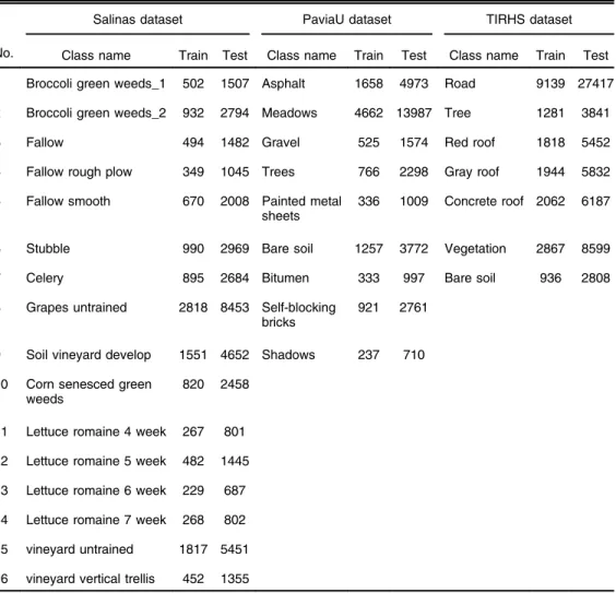
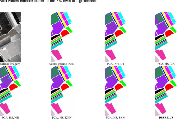
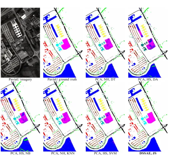
To evaluate the potential of the proposed hyperspectral imagery classification framework, two commonly used hyperspectral datasets (Salinas and PaviaU) and a coarse resolution hyperspec-tral dataset in the long-wave infrared range (LWIR) are investigated (as at-sensor radiance data). The Salinas scene (Fig.3) is of512×217pixels with 3.7-m spatial resolution. The 224 spectral band AVIRIS scene was collected over Salinas Valley, California. The data comes with a 16 class labeled ground truth map. Of the 224 bands, 20 spectral bands [(108–112), (154–167), and 224] were discarded due to their water absorption features. The Pavia University image (Fig.4) is of 610×340 pixelswith 103 bands at 1.3-m spatial resolution. The image was collected by the ROSIS sensor over Pavia, northern Italy, and the data is provided with a nine class labeled ground truth map. The LWIR hyperspectral imagery (Fig. 5) is of 874×751 pixels (with ∼1-mspatial resolution), and it was collected by a fixed-wing aircraft at∼800-mflight height over Thetford Mines in Québec, Canada. The data comes with a seven class labeled ground truth map. The LWIR hyperspectral imagery was acquired by the latest airborne LWIR hyperspectral imager“Hyper-Cam”containing 84 spectral narrow bands. In all the mentioned datasets, one-fourth of each ground truth label is randomly separated for training and the rest are used as the
testing samples (Table 1). In this section, comparative experiments are carried out on the described datasets to quantitatively investigate the superiority of the proposed spectral/spec-tral–spatial deep feature learning framework against the conventional classifiers,46 including
decision tree (DT), discriminant analysis (DA), naive Bayes (NB), K-nearest neighbor (KNN), and SVM. In the case of the conventional classifiers, Eigenvalue (EV), hyperspectral signal subspace identification by minimum error (HS), and noise-whitened Harsanyi–Farrand– Chang (NH) techniques10are adopted as intrinsic dimension estimation (IDE) to be used by dimensionality reduction with PCA.
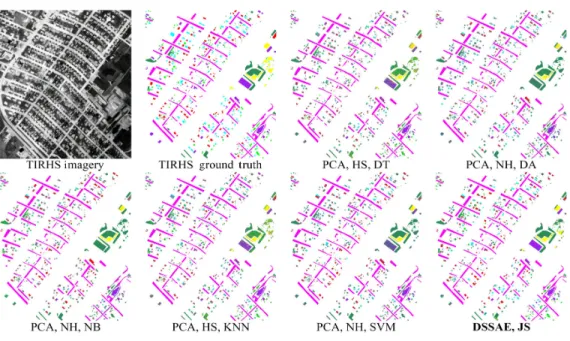
The first experiment is conducted on the Salinas hyperspectral imagery. To evaluate the pro-posed classification framework, a comprehensive comparison is performed via two quality indi-ces overall accuracy (OA) and kappa coefficient. The quantitative evaluation results obtained by the various classifiers are shown in Table 2. It can be seen that JS attains the most accurate classification result (OA/kappa: 98.07/97.85) compared with the conventional classifiers. Also, the visual inspection of the classification maps validates the effectiveness of the proposed classification technique (Fig.3). The second experiment is conducted on the PaviaU dataset. The implementation procedures are the same as that of the first dataset. As can be seen from Table3, JS obtains the highest classification accuracies (OA/kappa: 99.44/99.25). Figure4 shows the classification maps of the various classification frameworks. The last experiment is carried out on the TIRHS dataset. As per the classification results in Table4and by inspecting Fig.5, it can be seen that the JS classification framework provides again the best classification performance (OA/kappa: 80.70/73.58). Furthermore, Fig.6shows the quantitative evaluation results obtained by the various classifiers graphically.
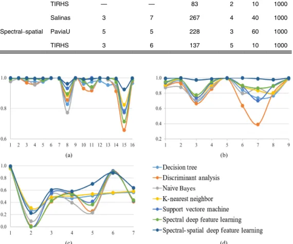
Table 1 Number of training and testing samples on different datasets.
No.
Salinas dataset PaviaU dataset TIRHS dataset Class name Train Test Class name Train Test Class name Train Test 1 Broccoli green weeds_1 502 1507 Asphalt 1658 4973 Road 9139 27417 2 Broccoli green weeds_2 932 2794 Meadows 4662 13987 Tree 1281 3841 3 Fallow 494 1482 Gravel 525 1574 Red roof 1818 5452 4 Fallow rough plow 349 1045 Trees 766 2298 Gray roof 1944 5832 5 Fallow smooth 670 2008 Painted metal
sheets
336 1009 Concrete roof 2062 6187
6 Stubble 990 2969 Bare soil 1257 3772 Vegetation 2867 8599 7 Celery 895 2684 Bitumen 333 997 Bare soil 936 2808 8 Grapes untrained 2818 8453 Self-blocking
bricks
921 2761
9 Soil vineyard develop 1551 4652 Shadows 237 710 10 Corn senesced green
weeds
820 2458
11 Lettuce romaine 4 week 267 801 12 Lettuce romaine 5 week 482 1445 13 Lettuce romaine 6 week 229 687 14 Lettuce romaine 7 week 268 802 15 vineyard untrained 1817 5451 16 vineyard vertical trellis 452 1355
Table 2 Salinas classification accuracies. No. PCA DSSAE EV HS NH EV HS NH EV HS NH EV HS NH EV HS NH DT DA NB KNN SVM SS JS 1 1.00 1.00 1.00 0.99 1.00 1.00 0.98 0.98 0.98 1.00 1.00 1.00 1.00 1.00 1.00 0.99 1.00 2 1.00 1.00 1.00 0.98 1.00 1.00 0.98 1.00 0.99 1.00 1.00 1.00 1.00 1.00 1.00 1.00 1.00 3 0.96 0.98 0.98 0.73 0.97 0.91 0.82 0.99 0.98 0.97 1.00 1.00 0.97 1.00 1.00 0.99 1.00 4 0.99 0.97 0.98 0.98 0.96 0.93 0.99 0.96 0.96 0.99 0.99 0.99 0.99 0.99 0.99 1.00 1.00 5 0.96 0.97 0.97 0.98 0.99 0.98 0.98 0.98 0.98 0.98 1.00 0.99 0.99 1.00 0.99 0.98 1.00 6 1.00 1.00 1.00 1.00 1.00 1.00 1.00 1.00 1.00 1.00 1.00 1.00 1.00 1.00 1.00 1.00 1.00 7 0.99 1.00 1.00 1.00 1.00 1.00 1.00 0.99 1.00 1.00 1.00 1.00 1.00 1.00 1.00 0.99 1.00 8 0.80 0.83 0.83 0.85 0.85 0.85 0.61 0.77 0.73 0.82 0.89 0.88 0.88 0.93 0.92 0.89 0.96 9 0.99 0.99 1.00 1.00 1.00 1.00 0.99 0.99 0.99 0.99 1.00 1.00 0.99 1.00 1.00 1.00 1.00 10 0.90 0.96 0.96 0.60 0.93 0.91 0.88 0.99 0.98 0.97 0.99 0.99 0.96 0.99 0.99 0.98 0.99 11 0.94 0.97 0.98 0.86 0.92 0.92 0.90 0.93 0.93 0.99 1.00 1.00 0.98 1.00 0.99 0.94 0.99 12 0.99 0.98 0.98 0.99 1.00 1.00 0.98 1.00 1.00 1.00 1.00 1.00 1.00 1.00 1.00 1.00 1.00 13 0.96 0.95 0.95 0.99 1.00 1.00 0.98 0.99 0.98 1.00 1.00 0.99 0.99 1.00 1.00 1.00 1.00 14 0.94 0.95 0.95 0.91 0.91 0.92 0.93 0.94 0.92 0.98 0.99 0.99 0.98 0.99 0.98 0.97 1.00 15 0.70 0.75 0.78 0.35 0.66 0.64 0.77 0.77 0.78 0.73 0.82 0.82 0.61 0.78 0.77 0.71 0.92 16 0.97 0.96 0.97 0.89 0.98 0.98 0.94 0.98 0.98 1.00 1.00 1.00 0.99 1.00 1.00 0.99 1.00 OA 0.90 0.92 0.92 0.84 0.91 0.90 0.86 0.91 0.90 0.92 0.95 0.95 0.92 0.95 0.95 0.93 0.98 kappa 0.89 0.91 0.92 0.82 0.90 0.89 0.85 0.90 0.89 0.91 0.95 0.94 0.91 0.95 0.94 0.93 0.98
Note: Number of intrinsic dimensionality: EV¼6, HS¼23, and NH¼14. Bold values indicate outlier at the 5% level of significance.
Table 3 PaviaU classification accuracies. No. PCA DSSAE EV HS NH EV HS NH EV HS NH EV HS NH EV HS NH DT DA NB KNN SVM SS JS 1 0.89 0.89 0.90 0.93 0.89 0.93 0.83 0.87 0.87 0.88 0.85 0.91 0.94 0.94 0.93 0.95 0.99 2 0.95 0.94 0.95 0.87 0.93 0.90 0.86 0.88 0.87 0.96 0.97 0.98 0.96 0.98 0.97 0.98 1.00 3 0.68 0.68 0.69 0.46 0.66 0.60 0.70 0.71 0.71 0.69 0.67 0.75 0.69 0.74 0.71 0.78 0.97 4 0.90 0.86 0.88 0.82 0.86 0.82 0.84 0.88 0.85 0.90 0.88 0.91 0.85 0.94 0.91 0.95 0.99 5 1.00 1.00 1.00 0.99 1.00 0.99 1.00 1.00 1.00 1.00 1.00 1.00 1.00 1.00 1.00 0.99 1.00 6 0.84 0.83 0.84 0.35 0.64 0.58 0.79 0.80 0.81 0.86 0.85 0.89 0.89 0.89 0.89 0.90 1.00 7 0.67 0.75 0.74 0.00 0.39 0.03 0.80 0.87 0.85 0.71 0.71 0.83 0.00 0.70 0.64 0.86 0.99 8 0.76 0.75 0.77 0.85 0.80 0.83 0.78 0.79 0.80 0.79 0.65 0.80 0.85 0.90 0.88 0.89 0.98 9 0.99 0.99 0.99 1.00 1.00 1.00 0.99 0.99 0.99 0.99 0.99 1.00 0.99 0.99 1.00 1.00 1.00 OA 0.89 0.88 0.89 0.77 0.85 0.82 0.84 0.86 0.85 0.90 0.88 0.92 0.89 0.93 0.92 0.94 0.99 kappa 0.85 0.84 0.86 0.69 0.79 0.76 0.79 0.81 0.81 0.86 0.84 0.90 0.85 0.91 0.90 0.92 0.99
Note: Number of intrinsic dimensionality: EV¼5, HS¼49, and NH¼9. Bold values indicate outlier at the 5% level of significance.
The overall results demonstrate that the proposed spectral–spatial deep feature learning framework outperforms the conventional classifiers in terms of classification metrics used. JS provides 2.67/2.98%, 6.10/8.13%, and 6.80/9.49% classification performance improvements for Salinas, PaviaU, and the TIRHS hyperspectral data, respectively, in terms of OA/kappa met-rics. It can be also seen that the accuracies of most classes have been increased effectively. Table5indicates the grid search hyperparameters for the proposed deep frameworks.
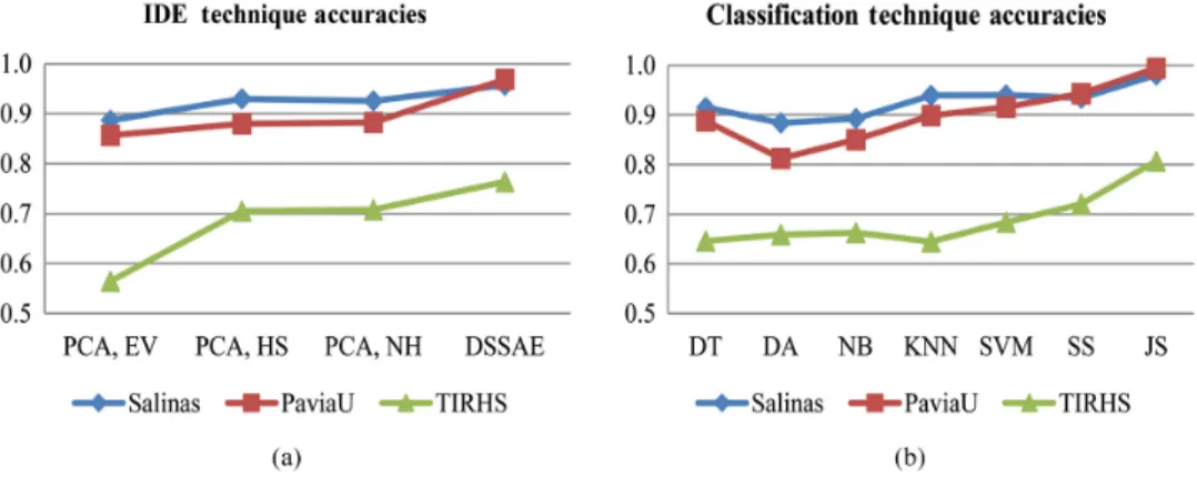
Figure7shows IDE techniques and the classifier’s average overall accuracy to summarize the obtained results. It is clearly obvious that the proposed classification procedure tends to be more robust and obtains the highest classification results in terms of the classification quality index.
Table 4 TIRHS classification accuracies.
No. PCA DSSAE EV HS NH EV HS NH EV HS NH EV HS NH EV HS NH DT DA NB KNN SVM SS JS 1 0.83 0.96 0.95 0.95 0.95 0.96 0.94 0.95 0.95 0.80 0.96 0.96 0.97 0.97 0.97 0.97 0.99 2 0.18 0.28 0.32 0.00 0.00 0.01 0.00 0.06 0.09 0.21 0.31 0.29 0.00 0.00 0.00 0.00 0.23 3 0.19 0.48 0.46 0.00 0.33 0.41 0.00 0.55 0.54 0.20 0.48 0.46 0.00 0.56 0.55 0.42 0.60 4 0.22 0.47 0.47 0.05 0.59 0.55 0.13 0.37 0.40 0.24 0.51 0.49 0.00 0.50 0.53 0.54 0.58 5 0.29 0.51 0.50 0.00 0.23 0.26 0.17 0.22 0.23 0.33 0.54 0.50 0.15 0.28 0.41 0.36 0.70 6 0.51 0.55 0.54 0.95 0.92 0.92 0.94 0.90 0.88 0.45 0.56 0.54 0.94 0.93 0.91 0.90 0.89 7 0.20 0.57 0.56 0.00 0.40 0.41 0.00 0.44 0.44 0.20 0.58 0.53 0.00 0.42 0.43 0.44 0.64 OA 0.54 0.70 0.70 0.58 0.70 0.71 0.59 0.70 0.70 0.52 0.71 0.70 0.59 0.72 0.74 0.72 0.81 kappa 0.36 0.59 0.59 0.36 0.58 0.60 0.39 0.58 0.58 0.35 0.61 0.59 0.37 0.62 0.64 0.62 0.74
Note: Number of intrinsic dimensionality: EV¼1, HS¼5, and NH¼13. Bold values indicate outlier at the 5% level of significance.
In this section, we evaluate a sparse autoencoder reconstruction and the sensitivity of a fea-ture learning scheme with respect to the sparsity parameter, execution time, and effect of model depth to avoid influencing outcomes. First, we investigate the quality of feature descriptors to reconstruct original data in different iteration epochs. Furthermore, a set of experiments is con-ducted to investigate the effect of the sparsity parameter on the classification performance. Figure 8 shows the reconstructed raw spectral input in 10, 100, and 1000 iteration epochs and the sensitivity of the feature learning scheme with respect to the sparsity parameter. It can be concluded that autoencoder can reconstruct raw spectra input progressively more accurate and retains increasingly more spectral information. It can be also observed that a feature learning scheme is relatively robust for higher values of the sparsity parameter, while the representation will become sparser with smaller values.
The execution time of the deep learning framework contains training and testing times. Training time denotes the time utilization of the learning stacked sparse autoencoder, classifi-cation layers, and fine-tuning the deep feature learning architecture. Figure 9shows how the training time changes with variation of model hidden layer neurons and iteration epoch param-eters. It can be noticed that the training time gently increases with the extension of the number of hidden layer neurons and iteration epochs.
Fig. 6 The quantitative evaluation results of (a) Salinas, (b) PaviaU, (c) TIRHS, and (d) graphs’ legend.
Table 5 Model parameters of the proposed deep feature learning frameworks on different datasets.
Classifier Dataset Local window size No. of PCs No. of features Layers Units Iteration
Salinas — — 204 3 40 1000
Spectral PaviaU — — 103 2 60 1000
TIRHS — — 83 2 10 1000
Salinas 3 7 267 4 40 1000
Spectral–spatial PaviaU 5 5 228 3 60 1000
Fig. 8 Sparse autoencoder evaluation for (a) reconstruction of a raw spectra input in different iteration epochs and (b) the effect of sparsity parameter on the classification performance.
Fig. 9 Comparison of training time with the variation of model parameters (a) Salinas, (b) PaviaU, and (c) TIRHS and comparison of testing time with the variation of model depths: (d) Salinas, PaviaU, and TIRHS Datasets.
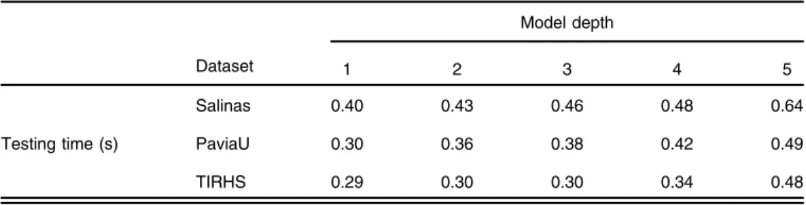
Moreover, a comparison of the testing times, for different model depths, is displayed in Table 6. The superiority of the proposed deep feature learning framework can be observed by looking at the superfast performance of the testing step.
In addition, model depth plays a significant role in the classification performance because it can improve the feature representation quality of the original data. In general, the higher model depths tend to extract more detailed representations of raw data. In this context, a set of experi-ments is carried out to evaluate how the depth parameter of the deep feature learning architecture shows an impact on the classification results (Table7). It can be concluded that the classification accuracy improves with the expansion of the model depth parameter and it also indicates that as the model depth keeps increasing, the accuracy tends to decline.
The overall results prove that the proposed spectral–spatial deep feature learning exhibits a superior classification performance for hyperspectral image data classification compared to the conventional spectral-based classification methods.
4 Conclusions
In this paper, joint spectral–spatial information is exploited in a deep stacked sparse autoencoder for hyperspectral imagery classification. Experiments and results show that the spectral–spatial feature descriptors improve the classification results compared with the spectral-based classi-fiers. Furthermore, the proposed classification framework provides statistically higher classifi-cation accuracy and appears to be more robust than the conventional classificlassifi-cation methods based on consistency over three hyperspectral datasets. We evaluated the sparse autoencoder reconstruction, execution time, and effect of model depth on hyperspectral imagery classifica-tion. In this context, we suggest using a deep learning model to obtain higher classification accuracy and consume the least amount of execution time. In future work, we will consider how to effectively employ textural features to enhance the classification results.
Acknowledgments
The authors would like to thank Telops Inc. (Québec, Canada) for acquiring and providing the data used in this study, the IEEE GRSS Image Analysis and Data Fusion Technical Committee and Dr. M. Shimoni (Signal and Image Centre, Royal Military Academy, Belgium) for organizing the 2014 Data Fusion Contest, the Centre de Recherche Public Gabriel Lippmann (CRPGL, Luxembourg) and Dr. M. Schlerf (CRPGL) for their contribution of the Hyper-Cam LWIR sensor, and Dr. M. De Martino (University of Genoa, Italy) for her contribution in data preparation.
Table 7 Comparison of overall accuracy for different model depths.
Dataset Model depth 1 2 3 4 5 Salinas 97.65 97.67 97.75 98.07 97.20 OA (%) PaviaU 99.29 99.39 99.44 99.32 99.15 TIRHS 78.39 79.21 79.34 79.82 80.70
Table 6 Comparison of testing time for different model depths.
Dataset
Model depth
1 2 3 4 5
Salinas 0.40 0.43 0.46 0.48 0.64
Testing time (s) PaviaU 0.30 0.36 0.38 0.42 0.49
References
1. S. Li et al.,“An effective feature selection method for hyperspectral image classification based on genetic algorithm and support vector machine,” Knowl.-Based Syst. 24(1), 40–48 (2011).
2. B. Bigdeli, F. Samadzadegan, and P. Reinartz, “A multiple SVM system for classifica-tion of hyperspectral remote sensing data,” J. Indian Soc. Remote Sens. 41(4), 763–776 (2013).
3. F. Samadzadegan, H. Hasani, and T. Schenk, “Simultaneous feature selection and SVM parameter determination in classification of hyperspectral imagery using ant colony opti-mization,”Can. J. Remote Sens. 38(2), 139–156 (2012).
4. P. Pahlavani and B. Bigdeli, “A mutual information-Dempster–Shafer based decision ensemble system for land cover classification of hyperspectral data,” Front. Earth Sci.
1–10 (2016).
5. V. N. Vapnik, Statistical Learning Theory, Wiley, New York (1998).
6. X. Jia, “Simplified maximum likelihood classification for hyperspectral data in cluster space,”inIEEE Int. Geoscience and Remote Sensing Symp. (IGARSS 2002), pp. 2578–2580 (2002).
7. P. K. Goel et al.,“Classification of hyperspectral data by decision trees and artificial neural networks to identify weed stress and nitrogen status of corn,” Comput. Electron. Agric.
39(2), 67–93 (2003).
8. G. Camps-Valls and L. Bruzzone,“Kernel-based methods for hyperspectral image classi-fication,”IEEE Trans. Geosci. Remote Sens.43(6), 1351–1362 (2005).
9. F. Del Frate et al.,“Use of neural networks for automatic classification from high-resolution images,”IEEE Trans. Geosci. Remote Sens.45(4), 800–809 (2007).
10. C.-I. Chang,Hyperspectral Data Processing: Algorithm Design and Analysis, John Wiley & Sons, Hoboken, New Jersey (2013).
11. C.-H. Li et al., “A spatial–contextual support vector machine for remotely sensed image classification,”IEEE Trans. Geosci. Remote Sens.50(3), 784–799 (2012).
12. L. Fang et al.,“Spectral–spatial hyperspectral image classification via multiscale adaptive sparse representation,”IEEE Trans. Geosci. Remote Sens.52(12), 7738–7749 (2014). 13. D. Akbari et al., “Mapping urban land cover based on spatial–spectral classification of
hyperspectral remote-sensing data,”Int. J. Remote Sens.37(2), 440–454 (2016).
14. L. Zhang, L. Zhang, and B. Du,“Deep learning for remote sensing data: a technical tutorial on the state of the art,”IEEE Geosci. Remote Sens. Mag.4(2), 22–40 (2016).
15. X. Chen et al.,“Vehicle detection in satellite images by hybrid deep convolutional neural networks,”IEEE Geosci. Remote Sens. Lett.11(10), 1797–1801 (2014).
16. Y. Chen et al.,“Deep learning-based classification of hyperspectral data,”IEEE J. Sel. Top. Appl. Earth Obs. Remote Sens.7(6), 2094–2107 (2014).
17. C. Tao et al.,“Unsupervised spectral–spatial feature learning with stacked sparse autoen-coder for hyperspectral imagery classification,”IEEE Geosci. Remote Sens. Lett.12(12), 2438–2442 (2015).
18. J. Yue et al.,“Spectral–spatial classification of hyperspectral images using deep convolu-tional neural networks,”Remote Sens. Lett.6(6), 468–477 (2015).
19. K. Makantasis et al.,“Deep learning-based man-made object detection from hyperspectral data,”inInt. Symp. on Visual Computing, pp. 717–727 (2015).
20. H. Liang and Q. Li,“Hyperspectral imagery classification using sparse representations of convolutional neural network features,”Remote Sens.8(2), 99 (2016).
21. C. Zhao et al.,“Spectral–spatial classification of hyperspectral imagery based on stacked sparse autoencoder and random forest,”Eur. J. Remote Sens. 50(1), 47–63 (2017). 22. L. Wang et al.,“Spectral–spatial multi-feature-based deep learning for hyperspectral remote
sensing image classification,”Soft Comput.21(1), 213–221 (2017).
23. S. Yu, S. Jia, and C. Xu,“Convolutional neural networks for hyperspectral image classi-fication,”Neurocomputing219, 88–98 (2017).
24. Y. LeCun, Y. Bengio, and G. Hinton, “Deep learning,” Nature 521(7553), 436–444 (2015).
25. A. Mohamed et al.,“Deep belief networks using discriminative features for phone recog-nition,” inIEEE Int. Conf. on Acoustics, Speech and Signal Processing (ICASSP 2011), pp. 5060–5063 (2011).
26. R. Collobert and J. Weston,“A unified architecture for natural language processing: deep neural networks with multitask learning,” in Proc. of the 25th Int. Conf. on Machine Learning, pp. 160–167 (2008).
27. Y. Bengio et al.,“Greedy layer-wise training of deep networks,”inAdvances in Neural Information Processing Systems, Vol. 19, pp. 153–160 (2007).
28. A. Krizhevsky, I. Sutskever, and G. E. Hinton,“Imagenet classification with deep convolutional neural networks,”inAdvances in Neural Information Processing Systems, pp. 1097–1105 (2012). 29. T. Serre et al.,“A quantitative theory of immediate visual recognition,”Prog. Brain Res.
165, 33–56 (2007).
30. Y. Freund and D. Haussler,“Unsupervised learning of distributions of binary vectors using two layer networks,”inAdvances in Neural Information Processing Systems(1994). 31. G. E. Hinton, S. Osindero, and Y.-W. Teh,“A fast learning algorithm for deep belief nets,”
Neural Comput. 18(7), 1527–1554 (2006).
32. D. E. Rumelhart, G. E. Hinton, and R. J. Williams,“Learning internal representations by error propagation,”Nature 323, 533–536 (1986).
33. P. Vincent et al.,“Extracting and composing robust features with denoising autoencoders,” inProc. of the 25th Int. Conf. on Machine Learning, pp. 1096–1103 (2008).
34. H. Lee et al., “Efficient sparse coding algorithms,” in Advances in Neural Information Processing Systems, Vol. 19, p. 801 (2007).
35. Y. LeCun et al.,“Gradient-based learning applied to document recognition,”Proc. IEEE
86(11), 2278–2324 (1998).
36. Y. Bengio et al.,“Learning deep architectures for AI,”Found. Trends®Mach. Learn.2(1), 1–127 (2009).
37. Y. Bengio, A. Courville, and P. Vincent,“Representation learning: a review and new per-spectives,”IEEE Trans. Pattern Anal. Mach. Intell. 35(8), 1798–1828 (2013).
38. W. Zhao et al.,“On combining multiscale deep learning features for the classification of hyperspectral remote sensing imagery,”Int. J. Remote Sens.36(13), 3368–3379 (2015). 39. Y. Chen, X. Zhao, and X. Jia,“Spectral–spatial classification of hyperspectral data based on
deep belief network,”IEEE J. Sel. Top. Appl. Earth Obs. Remote Sens.8(6), 2381–2392 (2015). 40. C. C. Tan and C. Eswaran,“Reconstruction of handwritten digit images using autoencoder neural networks,”inCanadian Conf. on Electrical and Computer Engineering (CCECE 2008), pp. 465–470 (2008).
41. G. E. Hinton and R. Salakhutdinov,“Reducing the dimensionality of data with neural net-works,”Science313(5786), 504–507 (2006).
42. X. Zhang et al.,“Fusing heterogeneous features from stacked sparse autoencoder for his-topathological image analysis,”IEEE J. Biomed. Health Inf.20(5), 1377–1383 (2016). 43. D. E. Rumelhart, G. E. Hinton, and R. J. Williams, “Learning representations by
back-propagating errors,”Cognit. Model. 5(1), 533–536 (1988).
44. D. C. Liu and J. Nocedal,“On the limited memory BFGS method for large scale optimi-zation,”Math. Program.45, 503–528 (1989).
45. E. D. Varga et al.,“Robust real-time load profile encoding and classification framework for efficient power systems operation,”IEEE Trans. Power Syst.30(4), 1897–1904 (2015). 46. L. I. Kuncheva, Combining Pattern Classifiers: Methods and Algorithms, 2nd ed., John
Wiley & Sons (2014).
Ghasem Abdireceived his BSc degree in geomatics engineering and his MSc degree in photo-grammetry engineering from the University of Tehran, Tehran, Iran, in 2009 and 2012, respectively. Currently, he is working toward his PhD in photogrammetry engineering at the University of Tehran, Tehran, Iran. His research interests include computer vision and pattern recognition, deep learning and machine vision, and image processing.
Farhad Samadzadeganreceived his PhD in photogrammetry engineering from the University of Tehran, Tehran, Iran, in 2001. Currently, he is working as a full professor in the Faculty of
Surveying and Geospatial Engineering at the University of Tehran, Tehran, Iran. He has more than 15 years of experience in designing and developing digital photogrammetric and remote sensing software and systems.
Peter Reinartz received his PhD in civil engineering from the University of Hannover, Hannover, Germany, in 1989. He is the head of the Department of Photogrammetry and Image Analysis, German Aerospace Centre (DLR), Remote Sensing Technology Institute, Wessling, Germany, and holds a professorship for geomatics with the University of Osnabrueck, Osnabrueck, Germany. He has more than 30 years of experience in image processing and remote sensing and over 400 papers in these fields.