Subjectivity analysis using machine learning algorithm

(1)

Page 1 of 85

Subjectivity Analysis Using Machine Learning

Algorithm

Erfan Ahmed – 13101139

Muhitun Azad - 13101073

Md. Tanzim Islam – 13101158

Md. Asad Uzzaman Sazzad – 13101152

Supervisor

Dr. Md. Haider Ali

Co-Supervisor

Samiul Islam

Department of Computer Science and Engineering

Fall 2016

(2)

Page 2 of 85

Declaration

We, hereby declare that this thesis is based on the results found by ourselves. Materials of work found by other researcher are mentioned by reference. This Thesis, neither in whole or in part, has been previously submitted for any degree.

Signature of Supervisor Signature of Author

____________________ ____________________

Dr. Md. Haider Ali Erfan Ahmed

Signature of Co-Supervisor Signature of Author

____________________ ____________________

Samiul Islam Md. Asad Uzzaman Sazzad

Signature of Author ____________________ Md. Tanzim Islam Signature of Author ____________________ Muhitun Azad

(3)

Page 3 of 85

Abstract

This paper investigates a new approach of finding sentence level subjectivity analysis using different machine learning algorithms. Along with subjectivity analysis sentiment analysis has also been shown separately in this work. Three different machine learning algorithms - SVM, Naïve Bayes and MLP have been used both for subjectivity and sentiment analysis. Moreover four different classifiers of Naïve Bayes and three different kernels of SVM have been used in this work to analyze the difference in accuracy as well as to find the best outcome among all the experiments. For subjectivity analysis rotten tomato imdb movie review [1] dataset has being used and for sentiment analysis acl imdb movie review [2] dataset has been used. Lastly, the impact of stop words and number of attributes in accuracy both for subjectivity and sentiment analysis has also been illustrated.

(4)

Page 4 of 85

ACKNOWLEDGEMENT

Our deep thanks to our thesis supervisor Dr. Md. Haider Ali and to our co supervisor Samiul Islam for their generous guidance and continuous support throughout the work.

We are extremely thankful to our parents, family members and friends for their support and encouragement.

Finally we thank BRAC University for giving us the opportunity to complete our BSc. Degree in Computer Science and Engineering.

(5)

Page 5 of 85

List of Figures

Figure No. & Name

Page No

3.1 WEKA Toolkit Graphical User Interface

24

3.2 Occurrence of ‘Amount’ in Train Set of Subjectivity

Analysis

25

3.3 Mean Value of ‘Amount’

26

3.4 Occurrence of ‘mel’ in Train File

26

4.1 Attribute Selection Figure

29

4.2 Work Flow

30

5.1 Hyper Plane in Scatter

32

5.2 Hyper Plane Margins Drawing

32

5.3 Finding Exact Hyper Plane Margin

32

5.4 Creating Two Class

33

5.5 Outline in Class

33

5.6 Hyper Plane Maximum Margin

33

5.7 Solving Problem with SVM

34

5.8 Naïve Bayes Classifier Example

37

5.9 Prior Probability Using Naïve Bayes

38

5.10 Single Layer MLP

41

5.11 Multiple Layer MLP

41

6.1 Accuracy Comparison (SVM Kernels)

45

6.2 Detailed Result (Poly Kernel)

46

6.3 Detailed Result (Normalize Poly Kernel)

46

6.4 Detailed Result (RBF Kernel )

47

(8)

Page 8 of 85

6.6 ROC=0.921 for Class S (Normalized Poly Kernel)

49

6.7 ROC=0.904 for Class S ( RBF Kernel)

49

6.8 Accuracy Comparison (Naïve Bayes Classifiers)

51

6.9 Detailed Result (Naïve Bayes Classifier)

52

6.10 Detailed Result (Bayes Net)

52

6.11 Detailed Result (Naïve Bayes Multinomial)

53

6.12 Detailed Result (Naïve Bayes Multinomial Updatable)

53

6.13 ROC=0.9204 for class S (Naïve Bayes)

55

6.14 ROC=0.9593 for class S (Naïve Bayes Net)

55

6.15 ROC=0.974 for class S (Naïve Bayes Multinomial)

56

6.16 ROC=0.974 for class S (Naïve Bayes Multinomial

Updatable)

56

6.17 Accuracy (MLP layer ‘o’)

57

6.18 Detailed Result (MLP layer ‘o’)

58

6.19 ROC=0.9283 for class S (MLP layer ‘o’)

59

6.20 Accuracy Comparison (Three Best Classifiers)

60

6.21 Accuracy Comparison (SVM Kernels)

64

6.22 Detailed Result (Poly Kernel)

65

6.23 Detailed Result (Normalize Poly Kernel)

65

6.24 Detailed Result (RBF Kernel)

66

6.25 ROC=0.948 for P (Poly Kernel)

67

6.26 ROC=0.948 for N (Poly Kernel)

67

6.27 ROC=0.9743 for P (Normalize Poly)

68

6.28 ROC=0.9743 for N (Normalize Poly)

68

6.29 ROC=0.972 for P (RBF)

68

(9)

Page 9 of 85

6.31 Accuracy Comparison (Naïve Bayes Classifier)

70

6.32 Detailed Result (Naïve Bayes Classifier)

71

6.33 Detailed Result (Naïve Bayes Net)

71

6.34 Detailed Result (Naïve Bayes Multinomial)

72

6.35 Detailed Result (Naïve Bayes Multinomial Updatable)

72

6.36 ROC=0.9582 for class P (Naïve Bayes)

74

6.37 ROC=0.9582 for class N (Naïve Bayes)

74

6.38 ROC=0.9559 for class P (Naïve Bayes Net)

74

6.39 ROC=0.9559 for class N (Naïve Bayes Net)

74

6.40 ROC=0.9698 for class P (Naïve Bayes Multinomial)

75

6.41 ROC=0.9698 for class N (Naïve Bayes Multinomial)

75

6.42 ROC=0.9698 for class P (Naïve Bayes Multinomial

Updatable)

75

6.43 ROC=0.9698 for class N (Naïve Bayes Multinomial

Updatable)

75

6.44 Accuracy (MLP layer ‘o’)

76

6.45 Detailed Result ( MLP layer ‘o’)

77

6.46 ROC=0.9471 for class P ( MLP layer ‘o’)

78

6.47 ROC=0.9471 for class N ( MLP layer ‘o’)

78

6.48 Accuracy Comparison (Three Best Classifiers)

79

6.49 Attribute VS Accuracy using Naïve Bayes Multinomial

Updatable

62

6.50 Attribute VS Accuracy using Naïve Bayes Multinomial

Updatable

(10)

Page 10 of 85

List Of Tables

Table No. & Name

Page No.

1 Evaluation on Test Set (SVM Kernels)

44

2 Detailed Accuracy Using Different Kernels

48

3 Evaluation on Test Set Using Different Classifiers

(Naïve Bayes)

50

4 Detailed Accuracy Using Different Classifiers of

Naïve Bayes

54

5 Evaluation on Test Set using MLP (layer ’o’)

57

6 Detailed Accuracy using MLP (layer ’o’)

58

7 Comparative Analysis (Three Best Classifiers)

60

8 Evaluation on Test Set Using Different Kernels

63

9 Detailed Accuracy using Different Kernels (SVM)

67

10 Evaluation on Test Set using Different Classifiers

69

11 Detailed Accuracy using Different Classifiers of

Naïve

Bayes

73

12 Evaluation on Test Set using MLP (layer ’o’)

76

13 Detailed Accuracy using MLP (layer ‘o’)

77

14 Comparative Analysis (Three Best Classifiers)

78

15 Stop Words Effect on Accuracy using Naïve Bayes

Multinomial Updatable Classifier

61

16 Stop Words Effect on Accuracy using Naïve Bayes

Multinomial Updatable classifier

(11)

Page 11 of 85

Abbreviations

SVM – Support Vector Machine

SMO - Sequential Minimal Optimization MLP – Multilayer Perceptron

NLP – Natural Language Processing S/O – Subjective / Objective

P/N – Positive / Negative

ICA - Iterative Collective Classification ILP - Integer Linear Programming

SWSD - Subjectivity Word Sense Disambiguation WEKA - Waikato Environment for Knowledge Analysis GUI - Graphical User Interface

TCL – Tool Command Language RBF – Radial Basis Function

(12)

Page 12 of 85

1. Introduction

1.1 Introduction

In the recent world of information sharing the interest in the field of automatic identification and extraction of opinions and sentiments in the text has increased to a great extent. These are widely used by the entrepreneur, product manufacturer, product users, politicians and many more. The manufacturers or the companies uses these opinion based forums for reviewing their products and the customers are using them to see others review on the products they are interested in. Some important place for finding opinions are blogs, social networking sites like Facebook, Twitter, online news portal etc. But in order to fulfill the purpose proper analysis of data is very important. The term subjectivity includes emotions, rants, allegations, accusations, suspicions and speculation and sentiment analysis includes the positive and negative opinions or comments. So in order to analyze the data the most important task is to identify Subjectivity and Sentiment properly. Many approaches to subjectivity analysis rely on lexicons of words that may be used to express subjectivity. Examples of such words are the following (in bold) [2]:

(1) He is a disease to every team he has gone to. (2) Converting to SMF is a headache.

(3) The concert left me cold. (4) That guy is such a pain.

If the system knows the meaning of these words then it can recognize the sentiment of these sentences whether the sentences have positive or negative stance. However these key words may have both subjective and objective meaning depending on the semantic orientation and context. This is called false hit – subjectivity clues used with objective senses. False hits cause significant errors in subjectivity and sentiment analysis. The following example contains all of the key words above but these are not used as a subjective sense. These are all false hits [2]:

(1) Early symptoms of the disease include severe headaches, red eyes, fevers and cold chills, body pain, and vomiting.

To minimize this kind of errors we choose sentence level classification. As depending on the sentences the meaning of words varies (s/o) we focus on sentences rather than individual words

(13)

Page 13 of 85 that express subjectivity. Additionally our dataset contains only movie reviews that reduces the variety of using a single keyword in a large scale.

In this work both subjectivity analysis and sentiment analysis have been conducted separately. First subjectivity analysis with rotten tomato imdb movie review [1] dataset has been shown. Second sentiment analysis with acl imdb movie review [2] has shown. Both of the analysis were done using three different machine learning algorithms – Naïve Bayes, SVM and MLP with their different classifiers, kernels and layer accordingly. With all the results of those experiments, a comparative analysis have been shown as well. Lastly the importance of stop words in both subjectivity analysis and sentiment analysis have been presented using Naïve Bayes algorithm.

1.2 Motivation

The main motivation for this task came from seeing the present demand and interest on data mining and opinion or emotion extraction. Public review or opinion on products helps both the manufacturer and the customers to know about the pros and cons of the product. In recent times it is observed that the opinions posting on social media helped to flourish the business and public sentiment and emotions created a great impact on political and social life. For instance sentiment analysis can help the politicians to check public reviews of their speech or activity and the government to make public survey on their newly ideas that will be implemented based on public review. Moreover the entrepreneurs or the producers can also be benefited by checking the review of their products from the public review and take necessary steps to implement better ideas with the help of subjectivity and sentiment analysis. Moreover it is important for a humanoid robotic system to understand human emotion to interact with human properly and for this subjectivity analysis is must needed.

1.3 Thesis Outline

Section 2 describes the background research and basic review about the topic. Section 3 describes terminology about what subjective and sentiment analysis is. It also describes the WEKA toolkit, its graphical user interface and working procedure. This is followed by methodology in section 4, where data collection, data formatting, attribute selection, algorithm selection and work flow is described. In section 5 it describes the algorithm is used in this research, which are SVM, Naïve Bayes and MLP. Section 6 describes the experiment and result

(14)

Page 14 of 85 analysis for both subject and sentiment analysis. Finally we conclude in section 8 along with our future work.

(15)

Page 15 of 85

2 Background Research

Deﬁnitions of subjective and objective is adopted from Akkaya C, Wiebe J, Mihalcea R. Subjective expressions are words or phrases that are used to express mental and emotional states, such as speculations, evaluations, sentiments, and beliefs. These states are generally termed as private state, an internal state that cannot be directly observed or veriﬁed by others. Polarity (also called semantic orientation) is also important to NLP applications. In review mining, we want to know whether an opinion about a product is positive or negative. [2]

Expressions may be subjective without having any particular polarity. An example given by Wilson J, Wiebe J, Hoffmann P, is “Jerome says the hospital feels no different than a hospital in the states”.

In addition, beneﬁts for sentiment analysis can be realized by decomposing the problem into Subjective or Objective(S/O) or neutral versus polar and polarity classiﬁcation.

The following subjective examples are given in [4]: His alarm grew.

alarm, dismay, consternation – (fear resulting from the aware- ness of danger)

=> fear, fearfulness, fright – (an emotion experienced in anticipation of some specific pain or danger (usually ac- companied by a desire to flee or fight))

What’s the catch?

catch – (a hidden drawback; “it sounds good but what’s the catch?”)

=> drawback – (the quality of being a hindrance; “he pointed out all the drawbacks to my plan”) They give the following objective examples:

The alarm went off.

alarm, warning device, alarm system – (a device that signals the occurrence of some undesirable event)

(16)

Page 16 of 85 to wear on your wrist”; “a device intended to conserve water”)

He sold his catch at the market.

catch, haul – (the quantity that was caught; “the catch was only 10 ﬁsh”) => indeﬁnite quantity – (an estimated quantity)

In the paper of Wiebe J, Mihalcea R it was showed how important is the interaction between subjectivity and meaning of the language. Moreover evidence was also given by them that subjectivity is a property that can be associated with word senses and word sense disambiguation can directly benefit from subjectivity annotations. To prove their hypothesis two questions were addressed, first is whether subjectivity labels can be assigned to word senses and secondly can an automatic subjectivity analysis be used to improve word sense disambiguation. To approach the first question two studies were performed, first annotators manually assign the labels subjective, objective or both to WordNet senses and secondly a method evaluates automatic assignment of subjectivity labels to word senses. An algorithm was devised to calculate subjectivity score and showed it can be used to automatically assess the subjectivity of a word sense. For the second question the output of a subjectivity sentence classifier is given as input to a word sense disambiguation system, which is in turn evaluated on the nouns from the SENSEVAL-3 English lexical sample task. In conjunction with ACL 2004 a workshop held in July 2004 Barcelona where Senseval - 3 took place in March-April 2004. Senseval-3 included 14 different tasks for core word sense disambiguation, multilingual annotations, subcategorization acquisition, logic forms, identification of semantic roles. The result of this experiment showed that subjectivity feature can significantly improve the accuracy of a word sense disambiguation system for those words that have both objective and subjective senses. The dataset used in this work was MPQA corpus having 10000 sentences from the world press annotated for subjective expressions. The MPQA Opinion Corpus contains news articles from a wide variety of news sources manually annotated for opinions and other private states (i.e., beliefs, emotions, sentiments, speculations, etc.). But the dataset were somehow seem to be worked as drawback because the annotations in the MPQA corpus works for subjective expressions in context thus the data is somehow noisy because objective senses may appear in subjective expressions [4].

In the research done by us an effective machine learning algorithms such as SVM(Support Vector Machine) and MLP(Multilayer perceptron)is used that generated more accuracy

(17)

Page 17 of 85 identifying subjectivity on a given context. The training dataset used is imdb rotten tomato movie review dataset. After identifying subjective sentence polarity was calculated – how much positive or negative sense they possess. Moreover for better accuracy the dataset were categorized into specific domains.

Many methods have been developed for subjectivity and sentiment analysis in previous works. Much earlier works were focused only in labeling unannotated word in a text by Church K. W, Hanks P [5] .

Another work was on automatically labeling of unannotated data done by Rilo? E, Wiebe J. First Hi-precision classifier was used by them to label unannotated data automatically that created a large training set. This training set was given to an extraction pattern learning algorithm similar to AutoSlog-TS. AutoSlog automatically builds dictionaries of extraction patterns for new domains. AutoSlog uses an annotated corpus and simple linguistic rules. A training corpus for AutoSlog must be annotated by a person to indicate which noun phrases need to be extracted from a text. AutoSlog-TS is the new version that generates dictionaries of extraction patterns using only preclassified texts, and does not require the detailed text annotations that AutoSlog did. The learned pattern that was obtained was used to identify more subjective sentences. However Hi-precision subjective classifier has a low recall rate which is only 31.9%. So AutoSlog-Ts won’t be used by us [6].

In another work Least Common Subsumer (LCS) was used for automatically word sense labeling done by Gyamfi Y, Wiebe J, Mihalcea R, Akkaya C. The features that exploits the domain information and hierarchical structure in lexical resources was used by them such as WordNet. Moreover other types of features were also used that measure the similarity of glosses and the overlap among sets of word that are related semantically. In this paper it was suggested by them that at first identifying subjective words and then disambiguating their senses would be an effective approach. Moreover it was also suggested that a layered approach where it was suggested to classify objective or subjective first and then classify the subjective instances by polarity (positive/negative). For obtaining better result domain was reduced to increase calculation speed. However SVM were used by us [7].

In order to model a discourse scheme to imporve opinion polarity classification a design choice had been investigated by Somasundaran S, Namata G, Wiebe J, Getor L. Supervised collective

(18)

Page 18 of 85 classification framework and unsupervised optimization framework was used by them. For supervised framework the classifier used was Iterative Collective Classification (ICA) and for unsupervised optimization Integer Linear Programming (ILP) was used. LU and Getoor approach were also used by them that predicts the class values using global and local features iteratively. Moreover the classifiers used in this paper supervised classifier, Local, are implemented using the SVM classifier from Weka toolkit and another supervised discourse-based classifier known as ICA was also implemented by SVM due to its relational classifier. ILP was implemented by using optimization toolbox from Mathworks and GNU Linear Programming kit. The main function of this work is only polarity classification where we worked on both subjectivity and polarity classification. Therefore we didn’t use this approach [8].

Another work was Review classification done by Turney P. D. In this work whether a review is positive and negative was being investigated. An unsupervised learning algorithm, PMI-IR was presented by him. The classification of a review is predicted by the average semantic orientation of the phrases in the review containing adjectives or adverbs. To classify review a part-of-speech tagger to extract phrase containing adjective was applied first then the PMI-IR algorithm was applied to estimate the semantic orientation. But PMI-IR algorithm is not efficient with data parsing. It takes only two consecutive words to classify a review as good or bad. What if the third word changes the resultant good review into a bad one? PMI-IR method is reliance on the number of results returned by Altavista, there is the possibility of the algorithm appearing better (and simpler) than it really is by implicitly using the search algorithms of Altavista because it indexes approximately 350 million web pages (only papers that are in english) . Altavista was chosen because it has a NEAR operator. The AltaVista NEAR operator constrains the search to documents that contain the words within ten words of one another, in either order. Previous work has shown that NEAR performs better than AND when measuring the strength of semantic association between words. But the problem is Altavista (presumably for speed purposes) does not generate all documents which match a query, but attempts to select the more relevant documents, it's probable that the results of the PMI-IR algorithm rely largely on Altavista's ranking algorithms. This likely makes the actual algorithm being used much more complicated. Despite the problem Altavista cannot be used anymore as the owner of Altavista, Yahoo has shutdown the company on June 28, 2013. Moreover the limitation of this work include the time required for queries and, for some applications, the level of accuracy that was achieved. The

(19)

Page 19 of 85 former difficulty will be eliminated by progress in hardware. The latter difficulty might be addressed by using semantic orientation combined with other features in a supervised classification algorithm. Considering all these limitations we will not use these algorithms [9]. Similar to review classification to find strong and weak opinion clauses three machine learning algorithms were used by Wilson T, Weibe J, Hwa Rebecca. Those are boosting, rule learning and support vector regression. The algorithms were used to train the classifiers, to determine the depth of the clauses to be classified, and the types of features used. The learning algorithm were varied by them in order to explore the effect of these algorithms on the classification. For boosting BoosTexture were used, for rule learning they Ripper were used and for support vector regression SVMlight were used. The data used for the classification and regression analysis were analyzed by Support vector machine. It(SVM) a is supervised learning model with associated learning algorithms. And SVM light is the implementation of SVM in C language.These algorithms SVMLight and BoosTexture were chosen because they have successfully been used for a number of natural language processing tasks [10].

Another work relating contextual polarity recognition was done which focused on phrase-level Sentiment Analysis done by Wilson T, Wiebe J, Hoffmann P. An approach of sentiment analysis were made by them that first determines whether an expression is neutral or polar and then disambiguates the polarity of the polar expressions whether the sentiment is positive or negative. With this approach, the system was able to automatically identify the contextual polarity for a large subset of sentiment expressions, achieving results that are significantly better than baseline. An annotation scheme was introduced on the MPQA corpus to tag the polarity such as positive, negative, both or neutral. To address the contextual polarity disambiguation they approached two step solution where the first step involves in determining polar or neutral content and in second step the context marked as polar in first step are taken under consideration to identify contextual polarity. For both steps classifiers were developed by using BoosTexter AdaBoost.HM machine learning algorithm with 5000 rounds of boosting. The classifiers are evaluated in 10 fold cross-validation experiments.

This paper works on just polarity classification where in our works are classifying both subjectivity objectivity and polarity so we didn’t find this approach effective for our experiment [11].

(20)

Page 20 of 85 Wiebe J, Mihalcea R.. Words were tagged with sense by them. First subjective and objective word were identified by them in a given corpora then they measure the polarity of the subjective sentences. They worked on contextual classification. The classifier used by them were Rule-based Classifier which is a sentence level classifier with high precision and low recall, Subjective/Objective Classifier which is a lexicon level classifier and Contextual Polarity Classifier which is also a lexicon level classifier. They established relation between sense subjectivity and contextual subjectivity. [2]

As our work is focused on the improvement of subjectivity and polarity classification we have used different machine learning algorithm for this purpose. First we have applied two different kernel of SVM – I) SMO poly kernel , ii) SMO normalized poly kernel. These two kernel gave us different results. After that we have applied Naive Bayes Model again with two different classifier of it – I) Multinomial naïve bayes, II) Multinomial Updatable naïve bayes. We have found significant difference using these algorithms with their different classifier and kernel selection.

Since imdb rotten tomato movie review data was used by us as our training data we believe that it will be more reliable than Altavista. As we are using SVM and Naive Bayes Model as our Subjective/Objective classifier so we believe it will be able to eliminate the possibility of bad data parsing and noticeable low recall rate.

(21)

Page 21 of 85

3 Terminology

3.1 Subjectivity Analysis

Subjectivity analysis means where the feeling of the individual taking part in the analysis process determines the outcome. Subjectivity is concept that relates personhood, reality and truth of various individuals. The term subjectivity most commonly used as an explanation of the perceptions, experiences, expectations, personal or cultural understanding and beliefs specific to a person, which is based on people judgment about truth or reality. It is often used in contrast of objectivity term. Objectivity is truth or realty which is free of any individuals influence. Subjectivity is a social mode that comes through innumerable interactions within society. Subjectivity is an individual process but it is also a process of socialization. People interact with everyone around the world. Subjectivity shapes in term of economy, political, community, opinion, as well as natural world.

3.2 Sentiment Analysis

Sentiment analysis means the use of NLP,text analysis to identify and find out subjective information and express fillings. It is also known as opinion boring, finding the attitude or opinion of a speaker. Sentiment analysis tries to determine the opinion of a speaker or a writer with respect to some subject or the overall circumstantial polarity of a document. It is widely used approach in social media and many other things to identify the opinion about an application.It’s a process of analysing the number of Likes, Shares or Comments you get on a product, post, opinion, music, and video to understand how people are responding to it. Was the review of the writer positive? Negative? Sarcastic? Ideologically biased?

Turney [12]and Pang [13] worked on this topic. Turney and Pang applied different methods to analyse the polarity of product reviews and movie reviews respectively. They have worked on document level. Pang and Snydey [14] find out the polarity of a document which can classify the document on a multi way scale. Pang worked with Lee [15] who expanded the task. They have classified the data of movie review as either positive or negative. On the contrary Snydey analysed and find out an in-depth analysis of restaurant reviews. He predicted ratings for various aspects of the given reviews on restaurants. The reviews were focused on the food and atmosphere of a particular restaurant. They suggested that in most statistical classification

(22)

Page 22 of 85

methods, neutral texts fiction near the binary classification boundary. Three categories must be found out in every polarity problem which was suggested by several researchers and they are positive, negative and neutral. Moreover, specific classifiers such as the SVMs or the Naïve Bayes can be benefited if there is a neutral class and it will improve the overall accuracy of the classification. There are two ways for operating with a neutral class. The first option is the algorithm starts with by first identifying the neutral language. Then filtering it out and then analysing the rest in terms of positive and negative sentiments. The second option is to build a three way classification in one step. This second approach often involves probability by which we will predict an outcome over all categories. A neutral class fully depends on the nature of the data whether to use it or not or how we can use it. If the data is clearly divided into three categories like neutral, negative and positive, then it is useful and easy for the classifier it we filter out the neutral language out and only focus on positive and sentiments. It will also make the work easy for the classifiers.

A different approach to find out the sentiment of a word is the use of a scaling system. Where words are associated with having a negative, neutral or positive sentiment where they are classified into groups like highest positive to highest negative with a given associated number on a -10 to +10 scale. It gives an opportunity to adjust the sentiment of a sentence with the surroundings of its environment. When we analyse a text or sentence with natural language processing, each word is selected and given a score a range of -10 to +10 based on the sentiment positive or negative words relate to the text and their associated scores. This gives us a more refined understanding of sentiment. Words which are negate that means which can be considered as negative words but they are not negative can affect the score of the sentiment. Alternatively, if we want to find out the sentiment in a text rather than the overall polarity of the text we can give text a positive or negative sentiment [16].

(23)

Page 23 of 85

3.3 WEKA

3.3.1 Background history

The full form of WEKA is Waikato Environment for Knowledge Analysis. It is worldwide popular software which is written in JAVA. It is a machine learning software. It was developed at the University of Waikato, New Zealand. It is a free software which is under the GNU General Public License. It is developed on almost machine learning algorithm to apply data mining task, by which one can find out the result easily. It is very easy to operate as it represents its own GUI (Graphical User Interface) where algorithms can easily applied directly. It also gives the option to call the algorithm from our own java code. WEKA contains tools for data pre-processing, classification, regression, clustering, association rules, and visualization.

3.3.2 Working procedure

WEKA is a worktable [17] which is represented in a GUI that contains various type of machine learning algorithm and different type of data mining tools that can analyse data and predictive simulation. The original non-Java version of WEKA was a TCL which is high level, general purposed dynamic programming language front-end to representing algorithms implemented in other programming languages. The original version which was designed using TCL was tool to analyse data from agricultural domains [18]. But in 1997 it was shifted fully to java based version which was named WEKA 3 is now used all around the world for different applications specially for educational and research purposes.

(24)

Page 24 of 85 Fig 3.1: WEKA Toolkit Graphical User Interface

WEKA is supported by several machine learning algorithms and standard data mining tasks. Data pre-processing, data classification, visualization, regression, clustering and feature selection these are few of those data mining tasks that weka can do. All of WEKA’s algorithms techniques are predicted by assuming that data is available as one relation. Here all the data point is described with fixed number of attributes. WEKA provides access to SQL data base servers using JAVA database connectivity and then it process the result and return it to data base query [19]. It is not capable of multi relation data mining. But there are options with separate software to convert a collection of database table and it convert it to a single table that is suitable for data processing in WEKA.

WEKA has a graphical user interface which is called Explorer is the easiest way to use it. This gives access to all of its facilities of WEKA just by selecting the proper algorithm and process by which we can see our desired output. For example, we can quickly give in a dataset through a file and build a decision tree from it. The Explorer helps us by showing every option on the user

(25)

Page 25 of 85 interface by only clicking on a particular option. Helpful tool tips pop up as the mouse passes over items on the screen to explain what they do. With a minimum effort we can get a result so easily but to understand the proper result how it came and what the process that generate the results are, we will have to understand those. A fundamental disadvantage of the Explorer is that it holds everything in main memory. Whenever we open a data set it automatically load everything at once. That results in that this process can be applied to small to medium sized problem. However, there are some algorithms we can operate large amount of data using those, which takes longer time but gives an output [17].

3.4 String To Word Vector

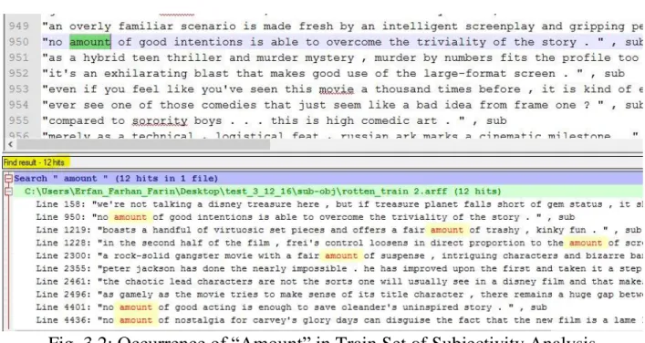
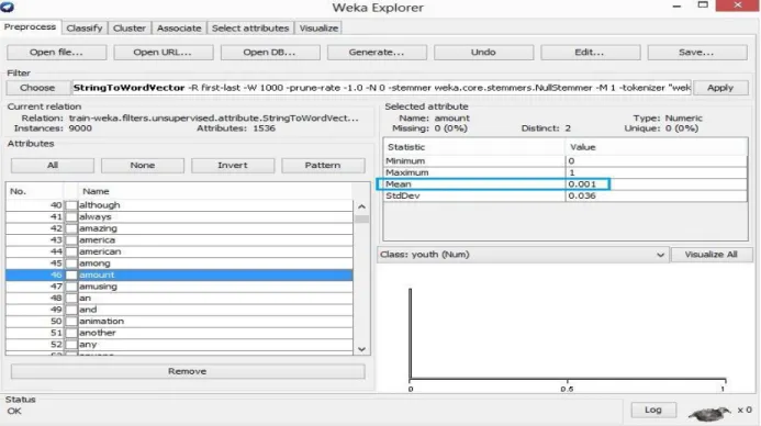
StringToWordVector is an unsupervised attribute filter built in java supported by WEKA toolkit that converts ALL the strings into a set of word vectors and choose each vector (unique word) as an attribute. We can also define the number of attributes we want to keep. By default WEKA takes 1000 attributes (form each class and selects the unique attributes among them) having higher mean value. We have conducted all the experiments with default settings. So as we get 1536 attributes from our training dataset. Among the attributes “amount” is taken as an attribute. In our training dataset “amount” - occurs 12 time and its mean value is .001 computed by StringToWordVector classifier.

(26)

Page 26 of 85

Fig.3.3: Mean Value of “Amount”

There is a word - “mel” in our train set. But this word has not been taken as an attribute because this word occurs only 6 times and has less mean value than .001.

(27)

Page 27 of 85 If we set the attribute number more than 1000 than more unique words will be chosen as

attributes having lower mean value. In a nutshell StringToWordVector Converts String attributes into a set of attributes representing word occurrence (depending on the tokenizer) information from the text contained in the strings.

(28)

Page 28 of 85

4 Methodology

4.1 Data collection

We have collected data from rotten tomato imdb movie review [1] for subjectivity analysis and acl imdb movie review [2] for sentiment analysis. There are 5000 subjective and 5000 objective instances separated in two text files in rotten tomato imdb movie review dataset. In acl imdb movie review dataset there are 12500 positive and 12500 negative reviews separated in two separated text file as well.

4.2 Data formatting

In our experiment we have modified the original data format and created a training and a testing dataset both in WEKA supported .arff format using Java code. First all quote (“ ”) characters, html tags were removed from the data set. Then quotes (“ ”) at the beginning and ending of each line of the dataset had been added. After that a comma (,) was put at the end of each line to separate the string and “sub” (without quote) for the subjective instances and “obj” (without quote) for the objective instances were added for the dataset of subjectivity analysis. For the dataset of sentiment analysis “pos” and “neg” were put at the end of each line of positive and negative instances respectively. Thus our training and testing dataset had been structured from the original dataset.

4.3 Attribute Selection

If “n” number of attribute is given in the WEKA GUI to be selected then what StringToWordVector does is, it takes “n” number of attributes with higher occurrence from each class. If any attributes matches it is counted as one attribute. In our case we had two class attributes. Following flow chart will give a clear view.

(29)

Page 29 of 85 Fig 4.1 Attribute Selection Figure

4.4 Algorithm selection

There are many machine learning algorithms for text classification as described in the literature review part. After days of researching SVM and Naïve Bayes have been found providing better accuracy in the case of classifying text with the dataset has been tested with. As SVM is a binary classifier it is better suited in classifying subjectivity and polarity of sentences. Since our work differentiate between subjective/objective and positive/negative sentences which is more likely to binary classification and SVM works better for it. Using Naïve Bayes algorithm instances can be classified more than two categories. Therefore it is also even more suitable using Naïve Bayes algorithm for classifying subjectivity and polarity of instances. In previous works subjectivity and polarity was being classified considering words, phrases, and semantic orientations but in our work the entire comment has been taken as a single instances that includes one or multiple lines of sentences. Therefore actually a lot of calculations and pre-processing have been reduced. As SVM and Naïve Bayes algorithm both works with numeric values not with strings, in our work each instance has been converted into word vector using WEKA’s built in unsupervised attribute filter- StringToWordVector. Moreover SVM has multiple kernel and Naïve Bayes has different classifiers which have provided us more options to test the dataset in different ways. Moreover MLP has also been tested with the dataset but much higher time complexity has been found than that of SVM and Naïve Bayes.

Give number of attributes (n) to be chosen

{(Choose n attributes from class A with higher occurrence) ⋃ (Choose n attributes from B with higher occurrence)}

(30)

Page 30 of 85

4.5 Work Flow

The following flow chart is given to show the overall procedure of our work.

Fig 4.2: Work Flow Build Model

Dataset collection Preprocessing Conversion to .arff

format

Creating train set Creating test set

Algorithm and classifier applied

(31)

Page 31 of 85

5 Machine learning algorithms

5.1 Support Vector Machine (SVM)

SVM (Support Vector Machine) is a machine learning algorithm. SVM is a supervised learning model which analyzes data for classification and regression analysis. SVM build a model using training algorithm that assigns new examples into one or two categories. SVM divided categories as wide as possible by creating a gap. New applications categories gap mapped into that same space or gap on which side the application fall on. The problem is when data are not properly labelled supervised learning is not possible. Then we have to follow an unsupervised learning approach to analyse, by which we can divide the data into separate groups. It follows a clustering approach which is called support vector clustering [20] and is often used in industrial applications either when data is not labelled or when only some data is labelled.

Example

Outlier: An outlier is an observation point that is distant from other observations.

An observation that is well outside of the expected range of values ina study or experiment, and which is often discarded from the dataset.

Hyper plane: In geometry a hyper plane is a subspace of one dimension less than its ambient space. If a space is 3-dimensional then its hyper planes are the 2-dimensional planes, while if the space is 2-dimensional, its hyper planes are the 1-dimensional lines. This notion can be used in any general space in which the concept of the dimension of a subspace is defined.

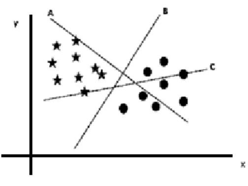
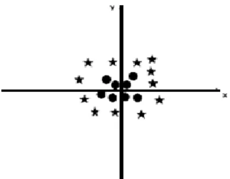
Suppose, we have three planes (A, B and C). Now, we need to identify the right plane to classify star and circle. We need to remember a thumb rule to identify the right hyper-plane.

(32)

Page 32 of 85 Fig 5.1: Hyper Plane in Scatter

Here, we have three hyper-planes (A, B and C) and all are in scatter possible ways. Now, how can we identify the right hyper-plane from these?

Fig 5.2: Hyper Plane Margins Drawing

Here, the distances between the nearest data point by maximizing and hyper plane will help us to decide the right hyper plane. This distance is called Margin.

Fig 5.3: Finding Exact Hyper Plane Margin

Above, we can see that the margin for hyper-plane C is high as compared to both A and B. Hence, we name the right hyper-plane as C. Another reason we should keep in mind that we have selected the hyper-plane with higher margin is robustness. [21]. Because if we select a

(33)

Page 33 of 85 hyper plane having low margin then there is a high chance is that there might be a miss classification of margin.

Fig 5.4: Creating Two Class

Here we are unable to differentiate the two classes using a straight line, as one of star is in the other class as an outlier.

Fig 5.5: Outline in Class

One star is in circle class which is an outlier and SVM has a kind of feature that can ignore the outliers and find the hyper plane that has maximum margin. Hence, we can say, SVM is husky to outliers.

(34)

Page 34 of 85 Here we can’t have linear hyper-plane between the two classes. SVM solves this problem by introducing additional feature. Here, we will add a new feature z=x^2+y^2 [21].

Fig 5.7: Solving Problem with SVM

SVM Applications

SVM is a tool for text classification which can reduce the need for labelled training examples in both standard inductive and tranductive settings. Image classification which is a part of image processing can also be performed using support vector machine. In the experiment and result analysis SVM achieve higher accuracy that other traditional schemes after almost just three or more round of feedback. To find out the image classification SVM follows same traditional approach as normal text analysis. The SVM algorithm has been also widely used in the biological and other sciences to find out results. SVM classifications have been used and it gives up to 90% of the compounds correctly. Support vector machine weights have also been used to consider SVM models in the past. Psthoc interpretation of support vector machine models has been used in order to identify features is a relatively new area of research with special significance in the biological sciences [22].

Sequential Minimal Optimization (SMO)

Sequential minimal optimization is a method of Support Vector Machine. It is an algorithm for solving the quadratic programming (QP) problem that arises during the training of support vector machines. SMO was invented by John Platt in 1998 at Microsoft Research. SMO is widely used

(35)

Page 35 of 85 for training support vector machines and is implemented by the popular LIBSVM tool, which is an open source machine learning library. After publication of SMO algorithm in 1998 it became easy to use SVM because previously used method were more complex and required quadratic programming solve.

max ∑𝑛_𝑖=1𝑎_𝑖 - 1⁄ ∑₂ _𝑖=1𝑛 ∑𝑛_𝑗=1𝑦_𝑖𝑦_𝑗𝐾(𝑥_𝑖, 𝑥_𝑗)𝑎_𝑖𝑎_𝑗, Subject to:

0≤ 𝑎_𝑖 ≤ 𝐶, for i = 1,2,…,n, ∑𝑛_𝑖=1𝑦_𝑖𝑎_𝑖 = 0

5.2 Naïve Bayes

In machine learning, naïve Bayes classifier is a simple probabilistic classifier which is based on Bayes theorem. It is a very popular method to categorize test, where the problem of judging text documents to one or more category with word frequencies as the feature. It is a machine learning algorithm which is with proper pre-processing it can be competitive methods like support vector machine. It can be also applicable for automatic medical diagnosis. Naïve Bayes classifiers are highly scalable, which requires linear number of variables. Maximum likelihood training can be done only by evaluating expressions taking linear amount of time. Other classifiers use expensive iterative approximation. Naïve Bayes is also called as Bayesand independent Bayes and many other different names. These names are the reference of the use of Bayes theorem in a classifier, but naïve Bayes is not one of the Bayesian methods. Naïve Bayes is a classifier method which uses a simple technique of constructing a classifier which represent as a vector feature values. In this case class labels are drawn from finite set. All naïve Bayes classifier assume that the value of a particular feature that is independent of any other feature. Thus Naïve Bayes is a full bunch of algorithm based on some common principles rather than a single algorithm.

(36)

Page 36 of 85

Naive Bayes is a conditional probability model. If we give a problem instance it will be represented by a vector

𝒙 = 𝒙

_𝟏,….,

𝒙

_𝒏 representing some n features, it assigns to this instance probabilities for each of K possible outcomes or classes

𝐶

_𝑘. [23]

(𝐶𝑘|𝑥1, … … , 𝑥𝑛)

But there is a problem with the above formula. The Problem is that if the number of features n is large or if a feature can take on a large number of values, then founding probability of this kind of table is difficult. We therefore reformulate the model to make it more feasible. Using Bayes Theorem, the conditional probability can be break down as

𝑝(𝐶_𝑘|𝑥) =𝑝(𝐶𝑘)𝑝(𝑥|𝐶𝑘) 𝑝(𝑥)

WE can also write the Bayesian theorem as:

𝑝𝑜𝑠𝑡𝑒𝑟𝑖𝑜𝑟 = 𝑝𝑟𝑖𝑜𝑟 × 𝑙𝑖𝑘𝑒𝑙𝑖ℎ𝑜𝑜𝑑 𝑒𝑣𝑖𝑑𝑒𝑛𝑐𝑒

But denominator does not depend on C the values of the features Fi are given, so that the denominator is constant. The numerator is equivalent to the joint probability model

𝑝(𝐶_𝑘,𝑥_1,……,𝑥_𝑛)

We can also write the equation as the definition of conditional probability: 𝑝(𝐶_𝑘,𝑥_1,……,𝑥_𝑛) = 𝑝(𝑥₁, … … , 𝑥_𝑛, 𝐶_𝑘)

= 𝑝(𝑥₁|𝑥₂, … . 𝑥_𝑛, 𝐶_𝑘) 𝑝(𝑥₂, … … , 𝑥_𝑛, 𝐶_𝑘)

= 𝑝(𝑥1|𝑥2, … . 𝑥𝑛, 𝐶𝑘) 𝑝(𝑥2|𝑥3, … . 𝑥𝑛, 𝐶𝑘) 𝑝(𝑥3, … … , 𝑥𝑛, 𝐶𝑘) = . . .

(37)

Page 37 of 85 Now assume that each feature Fi in conditionally independent of every other featureFjfor j != i ,

given the category C. This means that

𝑝(𝑥_𝑖|𝑥_𝑖+1, … . 𝑥_𝑛, 𝐶_𝑘) = 𝑝(𝑥𝑖|𝐶𝑘)

Thus, the joint model can be expressed as

𝑝(𝐶_𝑘|𝑥₁, … , 𝑥_𝑛) ∝ 𝑝(𝐶_𝑘, 𝑥₁, … , 𝑥_𝑛) ∝ 𝑝(𝐶𝑘)𝑝(𝑥1|𝐶𝑘)𝑝(𝑥2|𝐶𝑘)𝑝(𝑥3|𝐶𝑘)……

∝ p(𝐶_𝑘) ∏ 𝑝(𝑥_𝑖|𝐶_𝑘)

𝑛

𝑖=1

This means that under the above assumptions, the conditional distribution over the class variable C is : 𝑝(𝐶_𝑘|𝑥1, … … , 𝑥𝑛) = 1 𝑍𝑝(𝐶𝑘) ∏ 𝑝(𝑥𝑖|𝐶𝑘) 𝑛 𝑖=1

Where the evidence is Z = p(x) a scaling factor dependent only on , that is, a constant if the values of the feature variables are known.

Example Of Naïve Bayes

The Naive Bayes Classifier technique is based on the Bayesian technique. It is very suitable when the dimensionality of the inputs is high. It is a very simple method. But Naïve Bayes can perform elegant classification methods.

(38)

Page 38 of 85 Naïve Bayes Classification can be described by above figure. It indicates that the objects can be either GREEN or RED. This task is to find out which class they belong based on currently existing objects above.

Since there are twice as many GREEN objects as RED, it can possibly happen that a new class will have more GREEN than RED. In the Bayesian analysis it is called prior probability. Prior probabilities are often based on previous experience. It often can predict outcome before it actually happens.

Thus, we can write:

𝑃𝑟𝑖𝑜𝑟 𝑝𝑟𝑜𝑏𝑎𝑏𝑖𝑙𝑖𝑡𝑦 𝑓𝑜𝑟 𝐺𝑅𝐸𝐸𝑁 ∝𝑁𝑢𝑚𝑏𝑒𝑟 𝑜𝑓 𝐺𝑅𝐸𝐸𝑁 𝑂𝑏𝑗𝑒𝑐𝑡 𝑇𝑜𝑡𝑎𝑙 𝑁𝑢𝑚𝑏𝑒𝑟 𝑜𝑓 𝑂𝑏𝑗𝑒𝑐𝑡

𝑃𝑟𝑖𝑜𝑟 𝑝𝑟𝑜𝑏𝑎𝑏𝑖𝑙𝑖𝑡𝑦 𝑓𝑜𝑟 𝑅𝐸𝐷 ∝ 𝑁𝑢𝑚𝑏𝑒𝑟 𝑜𝑓 𝑅𝐸𝐷 𝑂𝑏𝑗𝑒𝑐𝑡 𝑇𝑜𝑡𝑎𝑙 𝑁𝑢𝑚𝑏𝑒𝑟 𝑜𝑓 𝑂𝑏𝑗𝑒𝑐𝑡

Since there is a total of 60 objects, 40 of which are GREEN and 20 RED, our prior probabilities for class membership are:

𝑝𝑟𝑖𝑜𝑟 𝑃𝑟𝑜𝑏𝑎𝑏𝑖𝑙𝑖𝑡𝑦 𝑓𝑜𝑟 𝐺𝑅𝐸𝐸𝑁 ∝40 60

𝑃𝑟𝑖𝑜𝑟 𝑃𝑟𝑜𝑏𝑎𝑏𝑖𝑙𝑖𝑡𝑦 𝑓𝑜𝑟 𝑅𝐸𝐷 ∝20 60

(39)

Page 39 of 85 Now we have a prior probability and now we can classify by adding a new object which is a WHITE Circle. These objects are well defined and we can assume that new object belong to a particular colour which is GREEN according to prior probability. To measure this likelihood, we draw a circle around X which includes a number of points irrespective of their class labels. Then we can calculate the number of points in the circle belonging to each class label. From this we calculate the likelihood:

𝐿𝑖𝑘𝑒𝑙𝑖ℎ𝑜𝑜𝑑 𝑜𝑓 𝑋 𝑔𝑖𝑣𝑒𝑛 𝐺𝑅𝐸𝐸𝑁 ∝ 𝑁𝑢𝑚𝑏𝑒𝑟 𝑜𝑓 𝐺𝑅𝐸𝐸𝑁 𝑖𝑛 𝑡ℎ𝑒 𝑣𝑖𝑐𝑖𝑛𝑖𝑡𝑦 𝑜𝑓 𝑋 𝑇𝑜𝑡𝑎𝑙 𝑁𝑢𝑚𝑏𝑒𝑟 𝑜𝑓 𝐺𝑅𝐸𝐸𝑁 𝑐𝑎𝑠𝑒𝑠

𝐿𝑖𝑘𝑒𝑙𝑖ℎ𝑜𝑜𝑑 𝑜𝑓 𝑋 𝑔𝑖𝑣𝑒𝑛 𝑅𝐸𝐷 ∝ 𝑁𝑢𝑚𝑏𝑒𝑟 𝑜𝑓 𝑅𝐸𝐷 𝑖𝑛 𝑡ℎ𝑒 𝑣𝑖𝑐𝑖𝑛𝑖𝑡𝑦 𝑜𝑓 𝑋 𝑇𝑜𝑡𝑎𝑙 𝑁𝑢𝑚𝑏𝑒𝑟 𝑜𝑓 𝑅𝐸𝐷 𝑐𝑎𝑠𝑒𝑠

From the above observation, it is clear that Likelihood of X given GREEN is smaller than Likelihood of X given RED, since the circle include only 1 GREEN object and 3 RED ones. Thus:

𝑃𝑟𝑜𝑏𝑎𝑏𝑖𝑙𝑖𝑡𝑦 𝑜𝑓 𝑋 𝑔𝑖𝑣𝑒𝑛 𝐺𝑅𝐸𝐸𝑁 ∝ 1 40 𝑃𝑟𝑜𝑏𝑎𝑏𝑖𝑙𝑖𝑡𝑦 𝑜𝑓 𝑋 𝑔𝑖𝑣𝑒𝑛 𝑅𝐸𝐷 ∝ 3

20

The prior probabilities indicate that X may belong to GREEN as there is twice as much GREEN than RED. But the likelihood indicates that the class membership of X is RED as the vicinity of RED is higher than the vicinity of GREEN. The final classification is produced by combining both sources of information, like the prior and the likelihood, to form a probability using the so-called Bayes' rule in Bayes Theorem. The probabilities are :

𝑃𝑜𝑠𝑡𝑒𝑟𝑖𝑜𝑟 𝑃𝑟𝑜𝑏𝑎𝑏𝑖𝑙𝑖𝑡𝑦 𝑜𝑓 𝑋 𝑏𝑒𝑖𝑛𝑔 𝐺𝑅𝐸𝐸𝑁 ∝ 𝑃𝑟𝑖𝑜𝑟 𝑃𝑟𝑜𝑏𝑎𝑏𝑖𝑙𝑖𝑡𝑦 𝑜𝑓 𝐺𝑅𝐸𝐸𝑁 × 𝐿𝑖𝑘𝑒𝑙𝑖ℎ𝑜𝑜𝑑 𝑜𝑓 𝑋 𝑔𝑖𝑣𝑒𝑛 𝐺𝑅𝐸𝐸𝑁

=

4 6

×

1 40

=

1 60

(40)

Page 40 of 85 𝑃𝑜𝑠𝑡𝑒𝑟𝑖𝑜𝑟 𝑃𝑟𝑜𝑏𝑎𝑏𝑖𝑙𝑖𝑡𝑦 𝑜𝑓 𝑋 𝑏𝑒𝑖𝑛𝑔 𝑅𝐸𝐷 ∝ 𝑃𝑟𝑖𝑜𝑟 𝑃𝑟𝑜𝑏𝑎𝑏𝑖𝑙𝑖𝑡𝑦 𝑜𝑓 𝑅𝐸𝐷 × 𝐿𝑖𝑘𝑒𝑙𝑖ℎ𝑜𝑜𝑑 𝑜𝑓 𝑋 𝑔𝑖𝑣𝑒𝑛 𝑅𝐸𝐷

=

4 6

×

1 40

=

1 60

Finally, we classify X as RED since its class membership achieves the largest probability [24].

5.3 Multilayer Perceptron (MLP)

Back propagation algorithm

Back propagation is a common method for training artificial neural network. It calculates gradient of loss function with respect to all the weight in a network. Each propagation implements in two steps forward and backward propagation.

MLP

A multilayer perceptron is an artificial feed forward neural network model. It maps sets of input data onto a set of appropriate outputs. It is a multiple layers of nodes directed graph where each layer is connected to the next one. The hidden nodes and the output notes are the processing elements with nonlinear activation function. Multilayer perceptron use back propagation algorithm [25]. Single propagation technique was invented by Rosenblatt in 1958. Multilayer perceptron performs generate a single output from multiple inputs by forming a linear combination. This linear combination based on input weights. [26]. Where W denotes the vector of weights, is the vector of inputs, is the bias and ø is the activation function.

𝑦 = ∅ (∑ 𝑤_𝑖𝑥_𝑖

𝑛

𝑖=1

(41)

Page 41 of 85 Fig 5.10: Single Layer MLP

A single perceptron where there is only a single layer is not very useful because of its limited mapping ability. Single perceptron uses different activation functions but it only able to represent an oriented ridge like function. A normal multilayer perceptron algorithm consists of a set of source nodes which form the input layer, one or more hidden layers of computation nodes, and an output layer of nodes. The input signal propagates layer-by-layer through the network [26].

5.11: Multiple Layer MLP

MLP network with one hidden layer can perform several other tasks. But they represent a rather limited kind of mapping. As Hornik and Funahashi showed in 1989 [27], such networks are capable of approximating any continuous function 𝑓: 𝑅𝑛 → 𝑅𝑚 to any given accuracy.

In supervised learning problems MLP are typically used. The supervised learning problem of the MLP can be solved with the back-propagation algorithm. The algorithm consists of two steps the forward and the backward pass. In forward pass, input we evaluate to determine the outcome.

(42)

Page 42 of 85 But in the backward pass, parameters are propagated back through the network weight. The network weights can then be adapted using any gradient-based optimisation algorithm. The whole process is iterated until the weights have converged [26]. The MLP network can also be used for unsupervised. Unsupervised learning can be done by setting the same values for both input and output networks. The sources emerge from the values of the hidden neurons [28]. The MLP network has to have at least three hidden layers for any reasonable representation and training such a network is a time consuming process.

(43)

Page 43 of 85

6. Experiment & Result Analysis

The results obtained from three machine learning algorithms with different classifiers and kernels are based on their accuracy, precision, recall, ROC area.

Recall is how many of the correct hits are found and Precision is how many of the returned hits are true positive means how many of the found are correct hits.

Precision is calculated using the formula, 𝑡𝑝

𝑡𝑝+𝑓𝑝

Recall is calculated using the formula, 𝑡𝑝 𝑡𝑝+𝑓𝑛

Where 𝑡𝑝 stands for true positive (actual and test data is correctly classified), 𝑓𝑛 stands for false negative (actual data is correct but predicted as incorrect), 𝑓𝑝 stands for false positive (actual is incorrect but predicted as correct).

F-measure is used to measure a test’s accuracy. F-measure can be interpreted as a weighted average of the precision and recall. F-score reaches best at 1 and worst at 0.

F-measure formula, 2 ·𝑝𝑟𝑒𝑐𝑖𝑠𝑖𝑜𝑛·𝑟𝑒𝑐𝑎𝑙𝑙

𝑝𝑟𝑒𝑐𝑖𝑠𝑜𝑛+𝑟𝑒𝑐𝑎𝑙𝑙

Receiver Operating Characteristic (ROC) or ROC curve is a graphical plot that illustrates the performance of a binary classifier system as its discrimination threshold is varied. The curve is created by plotting the false positive rate (FPR) along x-axis against the true positive rate (TPR) along y-axis at various threshold settings. Accuracy is measured by the area under the ROC curve. An area of 1 represents the perfect test and close to 1 is excellent test.

6.1 Subjectivity Analysis

9000 movie reviews containing 4500 subjective and 4500 objective instances for training set and 1000 movie reviews containing 500 subjective and 500 objective instances for test set was taken for subjectivity analysis.

(44)

Page 44 of 85

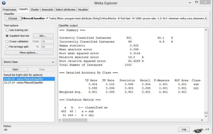
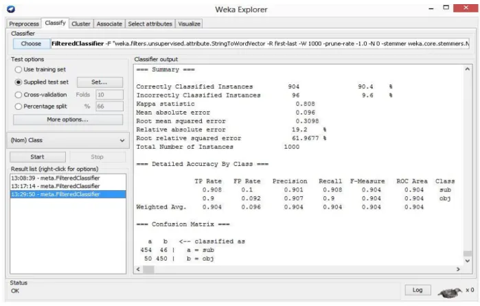
6.1.1 Experiment with SVM

As previously mentioned SMO classifier with three different kernels; Poly Kernel, Normalized Poly Kernel and Rbf Kernel was used for the experiment with SVM. Table 1 describes evaluation on test set using three different kernels of SVM. Figure 6.2, 6.3 and 6.4 was taken from the result window of WEKA which respectively represents three different kernels poly, normalize poly and rbf kernels output.

Algorithm Classifier Kernel Trained data Test data Correctly classified instances Incorrectly classified instances Accuracy Time to build model(s) SVM SMO poly kernel 9000 1000 901 99 90.1 66.95 SVM SMO normalized poly kernel 9000 1000 921 79 92.1 126.14 SVM SMO rbf kernel 9000 1000 904 96 90.4 98.38

(45)

Page 45 of 85 Fig 6.1: Accuracy Comparison (SVM Kernels)

In the above table 1, using poly kernel accuracy was achieved 90.1% where 901 instances were classified correctly and 99 instances classified incorrectly from 1000 test data. Then again using normalized poly kernel for the same test set accuracy increased 2 % from 90.1% to 92.1% where 921 instances were correctly classified and 79 instances were incorrectly classified. Changing kernel to RBF kernel for the same test set accuracy again decreased 1.7% from 92.1% to 90.4% than normalized poly kernel but increased only 0.3% from 90.1% to 90.4% than poly kernel where 904 instances were correctly classified and 96 instances were incorrectly classified. Though time taken to build model is highest in normalized poly kernel than two other kernels shown in table 1 but as this experiment is more concerned about accuracy so normalized poly kernel is the most successful than two other kernels used for the experiment with SVM. Figure 6.1 shows accuracy comparison using three different kernels.

90.1 92.1 90.4 89 89.5 90 90.5 91 91.5 92 92.5

poly kernel normalized poly kernel

rbf kernel

(46)

Page 46 of 85 Fig 6.2: Detailed Result (Poly Kernel)

(47)

Page 47 of 85 Fig 6.4: Detailed Result (RBF Kernel )

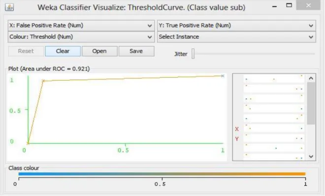
Table 2 describes the detailed accuracy using three different kernels where only weighted average of subjective and objective classes for different ratio is shown. In table 2, among all three kernels 𝑡𝑝 rate 0.921 is the highest which is in normalized poly kernel and 𝑓𝑝 rate 0.079 is also the lowest in normalized poly kernel. Precision, recall, f-measure and ROC area 0.921 is also highest in normalized poly kernel comparing to other two kernels. Here in table 2, area under the ROC curve 0.921 is the highest that means among all three kernels of SVM that was used to test, normalized poly kernel gives more accuracy to correctly classify the test set between two classes subjective and objective. Figure 6.5, 6.6 and 6.7 respectively represents the ROC curve of three different kernels poly, normalize poly and rbf which shows the ROC curve for subjective class. All these figures were taken from WEKA classifier visualize: threshold curve window where x-axis denotes false positive rate and y-axis denotes true positive rate.

(48)

Page 48 of 85

Kernel TP rate FP rate Precision Recall F-Measure ROC Area

poly kernel 0.901 0.099 0.901 0.901 0.901 0.901

normalized poly kernel

0.921 0.079 0.921 0.921 0.921 0.921

rbf kernel 0.904 0.096 0.904 0.904 0.904 0.904

Table 2: Detailed Accuracy Using Different Kernels

(49)

Page 49 of 85 Fig 6.6: ROC=0.921 for Class S (Normalized Poly Kernel)

(50)

Page 50 of 85

6.1.2 Experiment with Naïve Bayes

For Naïve Bayes experiment 4 different classifiers were used; Naïve Bayes, Bayes net, Naïve Bayes multinomial and Naïve Bayes multinomial updatable. Table 3 describes evaluation on test set using four different classifiers of Naïve Bayes and figure 6.8 shows the bar chart comparing accuracy of four different classifiers. Figure 6.9, 6.10, 6.11and 6.12 was taken from the result window of WEKA which respectively represents four different classifiers Naïve Bayes, Bayes net, Naïve Bayes multinomial and Naïve Bayes multinomial updatable outputs.

Algorithm Classifier Trained data Test data Correctly classified instances Incorrectly classified instances Accuracy Time to build model(s) Naïve Bayes Naïve Bayes 9000 1000 849 151 84.9 6.51 Naïve Bayes Bayes net 9000 1000 897 103 89.7 8.56 Naïve Bayes Naïve Bayes multinomial 9000 1000 926 74 92.6 0.52 Naïve Bayes Naïve Bayes multinomial updatable 9000 1000 926 74 92.6 0.45

Subjectivity analysis using machine learning algorithm