Study of separation phenomenon in transonic flows produced by interaction between shock wave and boundary layer

STUDY OF SEPARATION PHENOMENON IN

TRANSONIC FLOWS PRODUCED BY INTERACTION

BETWEEN SHOCK WAVE AND BOUNDARY LAYER

Hanoi University of Technology

Abstract. _{For compressible flows, the transonic state depends on the geometry, Mach}

number and the incidence. This effect can produce shock wave. Some studies showed that the interaction between shock wave and boundary layer concerns separation phenome-non. Studies in this report demonstrate conditions of separation in transonic flow and that it is not any interaction between shock wave and boundary layer which can cause boundary layer separation. The studies also show that maximum Mach number in the local supersonic region is not a unique factor influencing the separation, and the sepa-ration in transonic flows can occur at the incidence of 0o

. For the calculation of viscous transonic flows, we use Fluent software with serious treatment of application operation based on the physical nature of phenomenon and the technique of numerical treatment. For the calculation of invicid transonic flows, we built a code solving the full potential equation with verification for accuracy. Results calculated from Fluent have been seri-ously compared with results of present program and published results in order to assure the accuracy of application operation in the domain of investigation.

Key words:Separation in transonic flows, shock wave and boundary layer.

1. INTRODUCTION

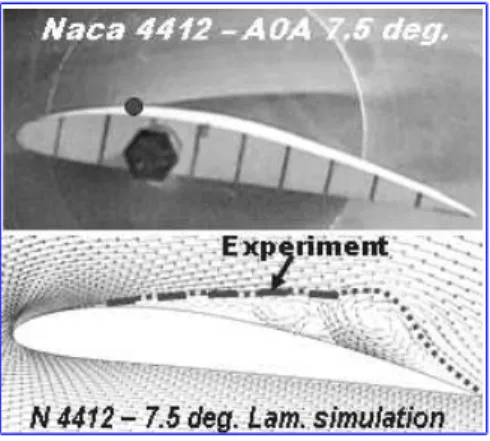
For incompressible flows, the laminar flow regime is very sensitive to boundary layer separation. Our experimental study [1], [8] showed that the laminar separation has appeared at very small incidence, at 2o _{or 3}o _{for profiles Naca 4412 and Naca 0012.}

Figure 1 presents experimental results in comparison with computational simulation on laminar separation for profile Naca 4412 with the incidence of 7.5o _{and Reynolds number}

Re= 13000.

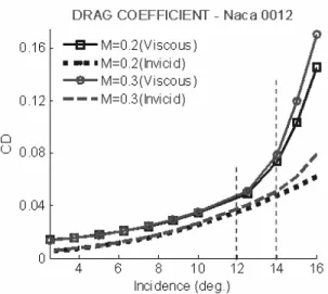
In the turbulent regime of incompressible flow, the separation occurs for profile Naca 0012 at angles of attack being greater than 12 degrees (and for profile Naca 4412 at angles of attack being greater than 10 degrees). Results of viscous calculation on the lift coefficient for profile Naca 0012 in Fig. 2 show that from 14o_{and more the lift coefficient}

decreases with downs of the lift graph, while results of invicid calculation show a quasi-linear increase of lift coefficient line. Results on the drag coefficient are presented in Fig.

Fig. 1. Laminar separation experimental and numerical results

3, and from 14o _{and more, the drag coefficient of viscous calculation strongly increases}

and very much differs from the one of invicid calculation.

Fig. 2. Lift coefficient of incompressible flows (Naca 0012)

For compressible flows, once the transonic phenomenon appears, separation laws are not similar to those of turbulent incompressible flows. The separation in transonic flows can occur at very small incidence, even at zero degree for symmetric profile (Naca 0012). This kind of separation depends on the interaction between boundary layer and shock wave. When transonic flow separation occurs results calculated by viscous and invicid flow theories are very different. The calculation of viscous transonic flow is carried out by using Fluent software in comparison with others which will be presented in the next part.

Fig. 3. Drag coefficient of incompressible flows (Naca 0012)

2. CALCULATION METHODS AND VERIFICATIONS

In order to study the transonic flow separation, it is necessary to solve viscous transonic flow problem. We built a code for calculation of invicid transonic flow by solving the full potential equation. And for viscous flow, we use Fluent software. However, Fluent is a code built by others. Its application operations need thus serious verifications.

The full potential equation (FPE) is writen [2]:

a2−_u2_φxx−2_uvφxy+ _a2−_v2_φyy = 0 (1) where φ is the velocity potential, u and v are velocity components; a is local velocity of sound.

The boundary condition of slid is imposed on the wall. At infinity, in cases having lift, the disturbance potetialϕ depends on the circulationΓ as follows:

ϕ= Γ 2π tan −1p 1−M2 ∞ y x (2) The equation (1) is a nonlinear second order partial differential equation for φ. If u2 +v2 < a2, this equation is elliptic, it is hyperbolic with u2 +v2 > a2 and parabolic with u2_+v2 _=a2_{. Set q}2 _=u2_+v2_{, on the grid of finite differences, at the point (i, j),} the full potential equation becomes:

a2−_u2_φxx−2_uvφxy+ _a2−_v2_φyy i,j− − a2−q2 i,j∆x u2 q2φxxx+ uv q2φxxy i,j − a2−q2 i,j∆y v2 q2φyyy+ uv q2φxyy = 0. (3) The first term in the equation (3) corresponds with differences in subsonic regions, and the two last terms correspond with differences in supersonic regions. The resolution of the equations (3) has been presented in [3]. This report represents the comparison of

results calculated from established program (FPE) and results calculated from Fluent in order to verify the operation of Fluent in domains for which the built program is unable to use.

2.1. Comparison of numerical and experimental results for flows without shock wave and with weak shock wave

For flows without shock wave and with weak shock wave, pressure coefficients cal-culated from viscous and invicid flows are not very different [4]. Following comparisons have been realized to verify operations of viscous flow calculation by using Fluent software in the mentioned domain.

Fig. 4. Comparison of Laser measure result [1] and numerical results (FPE, Fluent)

Fig. 5. Comparison of FPE results and invicid - viscous results of Fluent

Fig. 4 presents the comparison of our experimental results measured by Laser [1] and numerical results calculated from FPE present program and from viscous Fluent on the pressure coefficient (Cp) for the case of profile Naca 0012, incidence 0o, free Mach number

M∞ = 0.1. For the incompressible problem, experimental resutls, viscous numerical and

invicid numeriacal results are similar.

In Fig. 5 the results on pressure coefficients calculated from FPE present program in comparison with results of invicid and viscous flows calculated from Fluent (for profile Naca 0012, incidence 2o_,M

∞= 0.75)are presented. Sub-figure on the right shows results

of FPE program on Mach field and iso-Mach lines. This is a case of flow having weak shock wave. It is observed that a similarity of results calculated from built code and from Fluent software.

2.2. Comparison of numerical and experimental results for flows with shock wave

For transonic flows having rather strong shock wave, results calculated by invicid and viscous theories are considerably different. Here, viscous transonic problems calculated by Fluent and theirs results have been compared with experimental results of Riegels [5]. Fig. 6 shows the comparison of result on coefficient calculated from viscous Fluent and experimental result of Riegels [5] for flow of free Mach number M∞ = 0.7 around

profile Naca 0018 with the incidence of 2.65o_{. This transonic flow with a weak shock wave}

has not a boundary layer separation.

Fig. 6. a) Cp - Comparison between experiment [5] and viscous Fluent b) Mach field - computational results (Naca 0018, A = 2.65o

,M∞= 0.7)

Results of cases having strong shock wave are presented in Figs. 7 and 8 with the comparison between result of viscous Fluent and experimental result of Riegels [5]. Pressure coefficients are in sub-figure a, and computational simulation is in sub-figure b. It is observed that for the two cases of flows around Naca 0012 (M∞=0.8; angle of

attack 2.89o_{)in Fig. 7 and around Naca 0009 (M}

∞=0.84; angle of attack 2.59

o_{)in Fig. 8,}

boundary layer separations occur just behind shock wave faces.

Results of comparison presented in Figs. 4 - 8 verify application operations for Fluent software in the limitation of viscous transonic flows past aerofoils with a necessary accuracy for the investigation.

Fig. 7. a) Cp - comparison between experiment [5] and viscous Fluent b) Mach field - computational results (Naca 0012, A = 2.89o

,M∞= 0.8)

Fig. 8. a) Cp - comparison between experiment [5] and viscous Fluent b) Mach field - computational results (Naca 0009, A = 2.59o

,M∞= 0.84)

3. ANALYSES OF SEPARATION PHENOMENA IN TRANSONIC

FLOWS

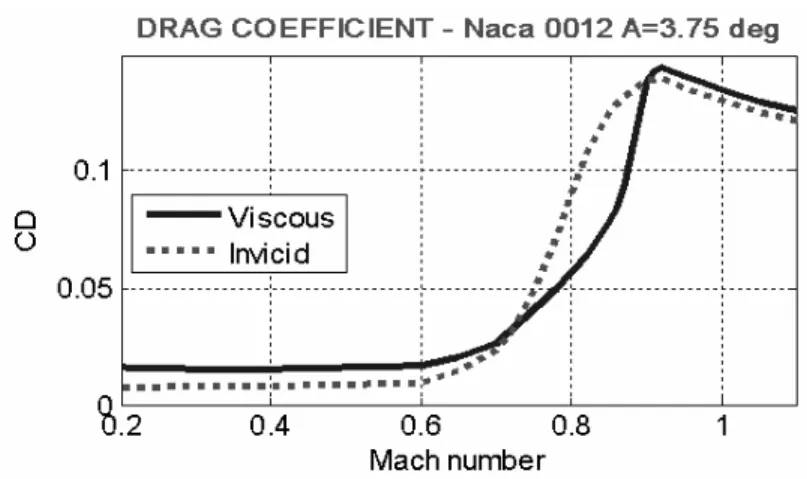
Fig. 9 shows numerical results on lift coefficient by using viscous and invicid theories for profile Naca 0012 with the incidence of 3.75o _{and free Mach number varying from 0.2}

to 1.1. Results on drag coefficient are presented in Fig. 10.

Transonic effect appears when free Mach numberM∞>0.3[6], [7] and it depends

on the incidence. For the case of profile Naca 0012 with the incidence of 3.75o_{, the transonic}

effect begins at free Mach numberM∞= 0.6. ForM∞>0.6, results calculated by viscous

and invicid theories have considerable differences. However, in the band ofM∞= 0.92−1.1,

lift coefficients and drag coefficients respectively become similar. Normally, for profile Naca 0012 at the angle of attackα= 3.75o_{, incompressible and subsonic compressible flows have}

Fig. 9. Lift coefficient - Naca 0012,α= 3.75o

Fig. 10. Drag coefficient - Naca 0012,α= 3.75o

Results in Figs. 9 and 10 show that aerodynamic characteristics are very different for viscous and invicid flow calculations with the band of free Mach number fromM∞= 0.73

to M∞ = 0.92 . Especially, for lift coefficient graph in Fig. 9, results of viscous flow

calculation have important downs in comparison with those of invicid flow calculation. We will realize analyses for cases: M∞= 0.7,M∞ = 0.8,M∞= 0.85,M∞ = 0.92(Naca

0012,α= 3.75o_).

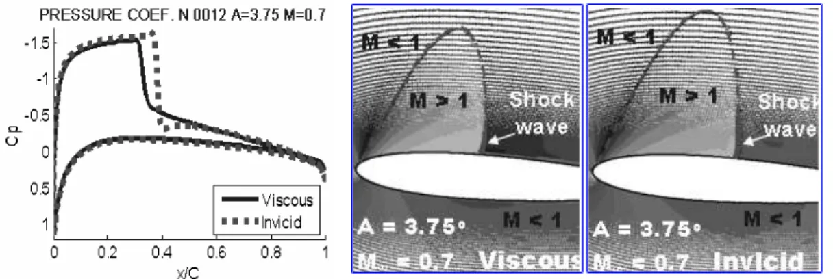
3.1. Physical phenomena for flow with free Mach number M∞= 0.7

In Fig. 11 the numerical results (pressure coefficient and field Mach) for the case of profile Naca 0012,α= 3.75o _{and M}

∞= 0.7are presented. On the profile lower, flows are

totally subsonic, pressure coefficients of viscous and invicid calculations are coincident. On the profile upper, there is a region of supersonic flow ending with a shock wave, pressure coefficients of viscous and invicid calculations are thus different, but not very great. The small difference can also seen in sub-figures of Mach fields when the supersonic region of

Fig. 11. Pressure coefficient and Mach field - Comparison between viscous and invicid calculations (Naca 0012,α= 3.75o

,M∞= 0.7)

invicid calculation is little greater than one of viscous calculation and the same for shock wave strength. Seeing in Fig. 9, the lift coefficient of invicid flow is 14% greater than the one of viscous flow.

The contours and areas of invicid and viscous supersonic regions are relatively sim-ilar for the case ofM∞ = 0.7. They become very different for regime ofM∞ = 0.8 which

will be considered in the next.

3.2. Physical phenomena for flow with free Mach number M∞= 0.8

For the case of M∞ = 0.8 in Fig. 12, pressure coefficients are totally different on

the upper side, and also different on the lower side of profile contour. Seeing in Fig. 9, the difference on lift coefficients of viscous and invicid flows is

δ = 0.833−0.38 0.5×(0.833 + 0.38)

≈75%.

Fig. 12. Pressure coefficient and Mach field - Comparison between viscous and invicid calculations (Naca 0012,α= 3.75o_,

M∞= 0.8)

The supersonic region of invicid flow is very bigger than one of viscous flow. But, it is more important that on the upper side there is a boundary layer separation behind shock wave face and the separation is not reattached on the profile. This separation causes the difference of lift coefficients on the lower side of viscous and invicid calculations in spite of flows on the lower side being subsonic in the two calculations.

The shock wave strength of viscous flow is much weaker than the one of invicid flow. Therefore, seeing in figure 10 at M∞= 0.8, total drag coefficient of viscous flow is lower

than drag coefficient of invicid flow. This is explained that in this case, shock wave drag is very much greater than friction drag.

Forms of supersonic regions become still very much more different for viscous and invicid flows when we consider the regime of free Mach numberM∞= 0.85 in the next.

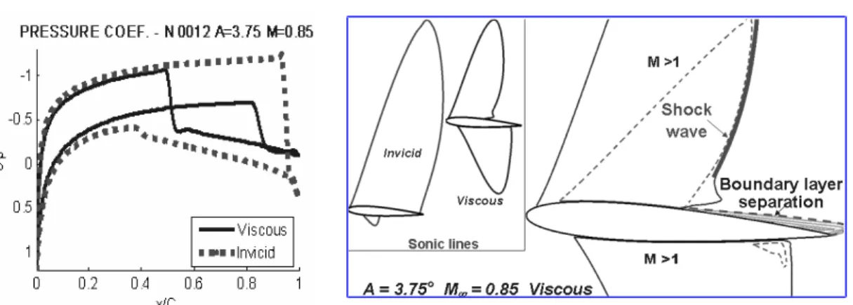
3.3. Physical phenomena for flow with free Mach number M∞= 0.85

Results on pressure coefficients and sonic lines for the case of M∞ = 0.85 are

presented in Fig. 13. In this case, pressure coefficients are totally different for viscous and invicid calculations. The difference is (see Fig. 9)

δ= 0.828−0.1254 0.5×(0.828 + 0.1254)

≈147%.

Fig. 13. Pressure coefficient and sonic lines - comparison between viscous and invicid calculations (Naca 0012,α= 3.75o

,M∞= 0.85)

Supersonic region contours of viscous flow totally differ from those of invicid flow. In addition, there is a boundary separation on the upper side of viscous flow which is not reattached on the profile contour. This phenomenon at trailing edge changes aerodynamic characteristics of viscous flow in comparison with flow using non-viscous hypothesis. Lift coefficient of viscous flow at M∞= 0.85has strong downs (see Fig. 9).

In the next part, we will consider other regime with free Mach number M∞= 0.92

to see the variety of gas-solid interaction in transonic flows.

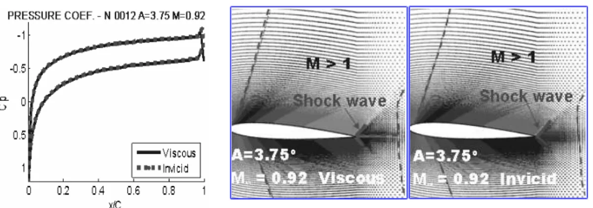
3.4. Physical phenomena for flow with free Mach number M∞= 0.92

In Fig. 14, it is observed that results on pressure coefficients and Mach fields are almost similar for viscous and invicid calculations.

Fig. 14. Pressurecoefficient and Mach field - Comparison between viscous and invicid calculations (Naca 0012,α= 3.75o

,M∞= 0.92)

For free Mach numberM∞= 0.92, on two sides of profile, supersonic regions occur

near leading edge and develop into the trailing edge. There is only oblique shock wave at trailing edge, and not on profile for both viscous and invicid calculations. In spite of high values of maximum Mach number (Mmax = 1.76 for viscous flow and Mmax = 1.86 for

invicid flow), because of having not shock wave on profile, boundary layer separation do not occur.

The physical phenomena are the same for flows having free Mach numbersM∞ = 0.92÷1.1. In this band of Mach number, aerodynamic characteristics of viscous and invicid flows are similar. This can be obverved in figures 9 and 10 on lift coefficients ans drag coefficients for regimes withM∞= 0.92÷1.1.

4. REMARKS FOR BOUNDARY LAYER SEPARATION PHENOMENA

IN TRANSONIC FLOWS

4.1. Boundary layer separation in transonic flow at incidence of 0o

At the certain Mach number, a boundary layer separation can occur at the incidence of 0o _{for an airfoil. Simulation results in Fig. 15 show boundary layer separations due to}

the interaction between shock wave and boundary layer on the two sides of profile Naca 0012 with free Mach number M∞= 0.87 and α= 0

o_.

4.2. Boundary layer separation non-concerning shock wave in transonic flow

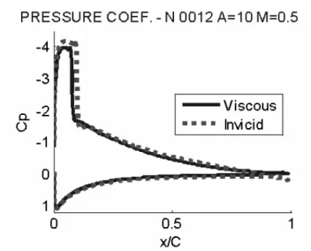
Consider the case of profile Naca 0012, M∞ = 0.5, α = 10

o _{in Fig. 16. There}

Fig. 16. Pressure coefficient (Naca 0012,α= 10o

,M∞= 0.5)

is a shock wave on the upper side at position x/C=0.1, with maximum Mach number Mmax= 1.53. In this case, there is not a boundary layer separation behind shock wave face,

but the one occurs at position x/C=0.83 and reattaches at x/C=0.98 on the upper side. This separation is not a consequence of the interaction between shock wave and boundary layer, but it is a normal separation at high incidence and free Mach number. Results on pressure coefficients of viscous and invicid calculations are thus not very different (in Fig. 16).

5. CONCLUSION

The above presented analyses of results permit to deduce some concluding remarks on physical properties of boundary layer separation in transonic flows which is produced by the interaction between shock wave and boundary layer:

- With a shock wave being sufficiently strong, the interaction between shock wave and boundary layer causes a boundary layer separation. That’s why the separation can be occurs at the incidence of 0o _{for an airfoil.}

- Once a separation due to the interaction between shock wave and boundary layer occurs, results on aerodynamic characteristics calculated by viscous and invicid theories are totally different.

- With a weak shock wave, the interaction between shock wave and boundary layer do not produce a separation, even the incidence is rather great. In these caces, pressure

coefficients and lift coefficients are respectively not very different for viscous and invicid calculations.

- The kind of separation produced by interaction between shock wave and boundary layer only appears for sub-transonic flows at a certain free Mach number which corresponds with a strong shock wave on profile. This condition is not satisfied for free Mach number very near to the unity and for sur-transonic flows, and there is not this kind of separation for flow regime at these free Mach numbers.

REFERENCES

[1] Hoang Thi Bich Ngoc, Nguyen Manh Hung, Velocity measurements on profile by means of laser measurer,Proceedings of National Conference on Metrology, Hanoi, (2010) 438-448. [2] Cole J. D., Cook L. P., Transonic aerodynamics,Elsevier Science Publishers B. V.,

Amster-dam, (1991).

[3] Hoang Thi Bich Ngoc, Le Hong Chuong, Numerical calculations by solving full potential equations, Proceedings of National Conference on Engineering Mechanics 2, Hanoi, (2006) 171-180.

[4] Hoang Thi Bich Ngoc, Bui Tran Trung, Nguyen Manh Hung, Simulation of transonic flows around profiles under invicid and viscous flow theories, Proceedings of National Conference on Engineering Mechanics 2, Hanoi, (2007) 379-388.

[5] Riegels F. W., Aerofoil sections,Butterworths, London, (1991).

[6] Hoang Thi Bich Ngoc, Influences of the compressibility on aerodynamic characteristics of profile under the transonic flow theory, Vietnam Journal of Mechanics, 29(4)(2007) 497-506.

[7] Hoang Thi Bich Ngoc, Study of transonic effect of flows around slender bodies of revolution and plane profiles,Vietnam Journal of Mechanics,32(1)(2010) 27-36.

[8] Nguyen Manh Hung, Hoang Thi Bich Ngoc, Experimental study of laminar separation phe-nomenon combining with numerical calculations,Vietnam Journal of Mechanics,33(2)(2011) 95-104.