kL-based Linear and Nonlinear Two-Equation Turbulence Models

kL-Based Linear and Nonlinear Two-equation

Turbulence Models

K. S. Abdol-Hamid

∗

Corresponding author: [email protected]

∗

_{NASA Langley Research Center, USA.}

Abstract

The development and implementation of kL-based Reynolds Average Navier-Stokes (RANS) two-equation turbulence models are reported herein. The kL is based on Abdol-Hamid’s closure and Menter’s modification to Rotta’s two-equation model. Rotta shows that a reliable transport equation can be formed from the turbulent length scale L, and the turbulent kinetic energy k. Rotta’s kL equation is well suited for term-by-term modeling and displays useful features compared to other scale formulation. One of the important differences is the inclusion of higher order velocity derivatives in the source terms of the scale equation. This can enhance the ability of RANS solvers to simulate unsteady flows in URANS mode. The present report documents the formulation of two model levels of turbulence models as implemented in the computational fluid dynamics FUN3D code. The levels are the two-equation linear k-kL and the two-equation algebraic Reynolds stress model (ARSM). Free shear, separated and corner flow cases are documented and compared with experimental, and other turbulence model data. The results show generally very good comparisons with experimental data. The results from this formulation are similar or better than results using the SST two-equation turbulence model. ARSM shows great promise with similar level of computational resources as basic two-equation turbulence models.

Nomenclature

H Heaviside function L turbulent length scale Lvk von K´arm´an length scale

M Mach number

Mt turbulent Mach number,

p

2k/a2 N number of nodes in grid

Pk production of turbulent kinetic energy PkL production of turbulent kL

Re Reynolds number

ReL Reynolds number based on length L S, Sij symmetric strain rate tensor ~

U, ui Cartesian velocity vector, (u, v, w)T

W, Wij asymmetric vorticity rate tensor a local speed of sound

b half width of stream, where (u−ue) is half of (um−ue)

c chord

cf local skin friction coefficient d distance normal to surface

f2 blending function for model corrections fc auxiliary function in compressibility model f(kL) auxiliary function in (kL) transport equation k turbulent kinetic energy

p pressure

r radius

T temperature

t time

ue edge velocity of outer co-flowing jet stream um peak velocity of co-flowing jet stream u+ velocity in wall units

xi Cartesian coordinates, (x, y, z)

y+ distance normal to surface in wall units 2D two-dimensional

3D three-dimensional

ARSM algebraic Reynolds stress model ARN acoustic research nozzle

CFD computational fluid dynamics C-D convergent-divergent

DNS direct numerical simulation LES large eddy simulation

NPR nozzle pressure ratio, pt,jet/p∞ RANS Reynolds averaged Navier-Stokes RSM Reynolds stress model

SAS Scale-Adaptive Simulation SST shear stress transport

URANS unsteady Reynolds averaged Navier-Stokes δij Kronecker delta

ε scalar dissipation κ von K´arm´an constant µ bulk viscosity

µt turbulent eddy viscosity

ρ density

τij Reynolds stress tensor 0 _{first derivative}

00 _{second derivative}

1

Introduction

T

hemechanism of the scale equation for determining turbulent length scale is not fully understood, and most formulations use a special boundary condition to simulate its wall boundary condition. Even the more complex model closures like Reynolds stress models (RSM) or explicit algebraic Reynolds stress models (ARSM) still use a scale equation. Almost all two-equation models use the turbulent kinetic energy, k, and its transport equation as one of the primary variables.

Historically, the modeling of the scale equation using dimensional arguments has been purely heuristic [1]. Many of the linear two-equation models for production use strain-rate or vorticity derived from the mean flow

terms, resulting in only one scale from the equilibrium of source terms for both equations. The scale equation is considered, in most cases, the weakest link in turbulence models, including much more complex approaches such as differential Reynolds stress and hybrid Reynolds Averaged Navier Stokes / Large Eddy Simulations (RANS/LES) formulations. It is difficult to justify using any of the complex turbulence models without fixing or using an alternate form for the scale transport equation. One of the few exceptions is the modeling concept proposed by Rotta [2], which can be formed as an exact transport equation for the turbulent length scale L. Rotta’s approach is well suited for term-by-term modeling and displays very favorable characteristics, as compared to other approaches. A key difference is the inclusion of higher-order velocity derivatives in the source terms of the scale equation. This potentially allows for resolution of the turbulent spectrum in unsteady flows.

Menter et al. [3–5] presented a complete detailed form of the k-√kL two-equation turbulence model based on the Rotta [2] approach. In Menter, it was proposed to replace the problematic third derivative of the velocity, that occurred in Rotta’s original model, with second derivatives of the velocity. Menter utilized this two-equation turbulence model to formulate the Scale-Adaptive Simulation (SAS) term that can be added to other two-equation models, such as Menter’s shear stress transport (SST) [6]. The SAS concept is based on the introduction of the von K´arm´an length scale into the turbulence scale equation. The information provided by the von K´arm´an length scale allows SAS models to dynamically adjust to resolved structures in unsteady RANS (URANS) simulations. This can create LES-like behavior in unsteady regions of flow fields. At the same time, the model provides standard RANS capabilities in stable flow regions.

Abdol-Hamid [7] documented an initial form of the k-kL two-equation turbulence model. He showed the process to calibrate the constants within the range suggested by Rotta [2] and satisfying the near-wall logarithmic requirements. It naturally contains the SAS characteristics through the von K´arm´an length scale. The basic model was implemented in the computational fluid dynamics (CFD) code Propulsion Aerodynamics Branch 3-Dimensional (PAB3D) [8]. A recent modification to the basic model referred to as k-kL-MEAH2015 turbulence model is documented in reference 9. The k-kL-MEAH2015 model has been implemented in the fully unstructured Navier-Stokes 3-Dimensional (FUN3D) code in a loosely coupled manner. For brevity, we will refer to k-kL-MEAH2015 as k-kL, herein. The implementation of k-kL in both CFL3D and FUN3D was verified in reference 9. Through private communication with researchers, Deutsches Zentrum fur Luft-und Raumfahrt e.V. (DLR) independently verified k-kL in its TAU CFD code. In reference 9, the results were compared with theory and experimental data, as well as with results using the SST turbulence model. The k-kL model was shown to produce results similar to or better than SST results. For example, for a separated axisymmetric transonic bump validation case, the size of the separation bubble (separation and reattachment locations) is better predicted by the k-kL model. Simulations have been carried out using five grid levels for the verification cases, avoiding grid refinement uncertainties. The validation results are compared with available experimental and/or theoretical data, depending upon the case. Most of the cases are taken from the turbulence modeling resource website [10, 11].

Subsonic and supersonic jet flows are quite difficult to predict with most RANS turbulence models. For subsonic jets, most turbulence models incorrectly predict the mixing rate so that the jet core length differs significantly from what is physically observed. The k-kL model also predicts a core length that is too short. A proposed jet correction, including compressibility effects, is described and is designated k-kL+J.

Theories for higher-order turbulence models such as RSM have been around for some time. The Launder Reece Rodi (LRR) [12] and Speziale Sarker Gatski (SSG) [13] are among the well known pressure-strain models. Hanjalic [14] provides a summary of different RSM. These models require much larger resources than two-equation turbulence models by adding five more equations. Other efforts are made to develop the ARSM based on SSG [13] that would require similar resources as general two-equation turbulence models. We will use the ARSM model that is fully documented and tested by Rumsey and Gatski [15] and Girimaji [16]. Another type of nonlinear model is introduced by Spalart [17] known as the Quadratic Constitutive Relation (QCR). These models have only had a minor additional impact to the overall computational effort and have the potential to resolve some of the errors and poor capabilities of linear turbulence models. The present paper documents the formulations of ARSM based on kL formulation. This model is compared with linear k-kL, other turbulence models and theoretical and experimental data that covers a wide range of flow complexity [18–22]. In general, ARSM shows the most promising results out of all the models presented here.

2

Computational Methods

FUN3D is an unstructured three-dimensional, implicit, Navier-Stokes code. Roe’s flux difference splitting [23] construction schemes include Harten-Lax-van Leer-Contact (HLLC) [24], upstream flux vector splitting (AUFS) [25], and Edwards’ low diffusion flux splitting scheme (LDFSS) [26]. The default method for calculation of the Jacobians is the flux function of van Leer [27]. The use of flux limiters are mesh- and flow-dependent. Flux limiting options include MinMod [28] and methods by Barth and Jespersen [29] and Venkatakrishnan [30]. Other details regarding _Fun3D can be found in Anderson and Bonhaus [31] and Anderson et al. [32], as well as in the extensive bibliography that is accessible at the _Fun3D web site, http://fun3d.larc.nasa.gov.

3

Turbulence Models Description

The kL length scale formulation is the base of the turbulence models presented in this section. The baseline k-kL turbulence model is described in section 3.1. The two-equation nonlinear ARSM based on kL is documented in section 3.2. The model to correct for free shear flows and compressibility effects is described in section 3.3.

3.1

Baseline two-equation k-kL Model

The k-kL two-equation turbulence model, equations 1 - 12, is based on Rotta’s k-kL approach with the modifications proposed by Menter [3–5] to develop a k-√kL model. A complete list of coefficients used by the present model is defined, where the third derivative of velocity was replaced with the second derivative of velocity. The closure constants were derived and documented by Abdol-Hamid [9].

∂ρk ∂t + ∂ρujk ∂xj =Pk+ ∂ ∂xj µl+σ(k)µt ∂ρk ∂xj −Cwµl k d2 −Ckρ k2.5 kL (1) ∂ρkL ∂t + ∂ρujkL ∂xj = C(kL₎₁ kL k PkL+ ∂ ∂xj µl+σ(kL)µt ∂ρkL ∂xj −6µlkL d2f(kL) −C(kL₎₂ρk1.5 (2)

The production of turbulent kinetic energy is stress-based (eq. 3) and is limited in both the k and kL equations (eq. 6).

Pk= P = τij ∂ui

∂xj (3)

The dissipation for the turbulence kinetic energy is ε=Ckρ

k2.5

(kL) (4)

The linear approach (L), for which stress is directly proportional to strain is as follows: τij=τ_ij(L)= 2µt Sij− 1 3tr{S}δij −2 3ρkδij (5) Sij = 1 2 _∂ui ∂xj +∂uj ∂xi , Wij = 1 2 _∂ui ∂xj −∂uj ∂xi

Pk =µtS2= 2µtSijSij, PkL= Pk = min P,20 Cµ3/4 ρk5/2 kL (6) with the turbulent eddy viscosity computed using equation 7:

µt= Cµ∗ Cµ C_µ1/4ρ(kL) k1/2 = Cµ∗ Cµ ρkτt (7)

Where,τt is the turbulent time scale defined as: τt=Cµ1/4

(kL) k3/2

For the linear approach, Cµ∗ = Cµ. The nonlinear ARSM model computes this coefficient as described in section 3.2. The functions and coefficients are:

Ck = Cµ3/4, C(kL₎₁=ζ1−ζ2A2L, AL = _kL kLvk , C(kL₎₂=ζ3 f(kL) = 1 + Cd1ξ 1 +ξ4 , ξ= ρ√0.3kd 20µ Lvk = κ U0 U00 , U0=p2SijSij, U00= s ∂2_u i ∂x2 k ∂2_u i ∂x2 j The second derivative expression of the velocity can be written out as:

U00 = s _∂2_u ∂x2 + ∂2_u ∂y2 + ∂2_u ∂z2 2 + _∂2_v ∂x2 + ∂2_v ∂y2 + ∂2_v ∂z2 2 + _∂2_w ∂x2 + ∂2_w ∂y2 + ∂2_w ∂z2 2 (8) The effective production of the kL in the equation is defined as:

PkL(ef f) =C(kL)₁ (kL) k PkL (9) where, C(kL)₁=ζ1−ζ2A2L, AL= L Lvk

The standalone Lvk has a singularity as U0 and U00 approach zero. Likely, Lvk is part ofPkL(ef f) and the AL terms of equation 9.

If(U00= 0andU0= 0), PkL(ef f) = 0 (10)

For all other conditions, following Menter et al. [3–5] with corrections proposed by Abdol-Hamid [7] for separated flow, we apply this limit on Lvk,

If(U00>0andU0≥0)

Lvk,min ≤ Lvk≤Lvk,max, Lvk,min= kL kC11, Lvk,max= C12κdfp fp = min max _PkkL C3/4_ρk5/2,C13 ,1.0 (11) The boundary conditions for the two turbulence variables, k and kL, along solid walls and the recommended

farfield boundary conditions for most applications are: kwall = (kL)wall= 0, k∞= 9×10 −10_a2 ∞, (kL)∞= 1.5589×10− 6µ∞a∞ ρ∞ (12) wherea∞ represents the speed of sound. The constants are:

σk = 1.0, σ(kL)= 1.0 κ = 0.41, Cµ= 0.09

ζ1 = 1.2, ζ2= 0.97, ζ3= 0.13

C11 = 10.0, C12= 1.3, C13= 0.5, Cd1= 4.7, Cw= 2.0

3.2

Nonlinear two-equation k-kL Model

Little data exist for implementing explicit ARSM using a generalized three-dimensional Navier-Stokes method such as_Fun3D. One approach is to develop algebraic relations with the tensorsT(λ) _as:

τij=τ_ij(ARSM)=−ρk aij+2 3δij =−ρk X βλT(λ)+2 3δij (13) These tensors are functions of strain, S, and vorticity, W, rates. Reference 33 shows the most general representation for a symmetric traceless second-order tensor, such asaij, which depends on two other second-order tensors, is a tensor polynomial containing ten tensorially independent groups,T(λ):

T(1)₌ S∗−1 3tr{S ∗_} , T(2)₌ S∗2₋1 3tr S∗2 T(3)₌ W∗2₋1 3tr W∗2 _{, T}(4) _{= [S}∗_W∗_−W∗_S∗_] T(5)=S∗2W∗−W∗S∗2, T(6)=S∗W∗2−W∗2S∗−2 3tr S∗W∗2 T(7)₌ S∗2_W∗2_+W∗2_S∗2₋2 3tr S∗2_W∗2∗ _{, T}(8)₌ W∗_S∗_W∗2 −W∗2_S∗_W∗ T(9)₌ W∗S∗W∗2−W∗2S∗W∗ , T(10)₌ W∗S∗2_W∗2_−W∗2_S2∗_W∗

3.2.1 Algebraic Model based on Full Reynolds Stress Model

In this section, we document ARSM based on RSM. For example, Wallin [33] described an ARSM that uses five tensors, (λ= 1, 3, 4, 6, and 9) that is based on the LRR turbulence pressure-strain model [12]. In the present report, we will focus on the cubic-based model from references [15] and [16] that are based on SSG [13]. We will refer to this model as k-kL-ARSM. This ARSM utilizes three tensors (λ= 1, 2, and 4) as follows: τ_ij(ARSM)=−ρk β1T(1)+β2T(2)+β4T(4)+ 2 3δij (14)

T(1)is the linear part of the model. However,T(2)andT(4)are the nonlinear terms that model the anisotropy. The coefficients for these terms are:

β1=−2Cµ∗= 2α, β2= 2a4a3β1, β4=−a4a2β1 (15) In this model,C_µ∗ is limited to be no smaller than 0.0005. For cubic based ARSM,αis the root of the cubic equation:

α3+pα2+qα+r= 0 (16)

where coefficients in equation 15 are defined as: a1= 1 2 ₄ 3 −C2 , a2= 1 2(2−C4) a3= 1 2(2−C3), a4=τ γ₁∗−2αγ₀∗η2τ2−1 (17)

We also use the following definitions and constants: τ = τt Cµ = Cµ1/4 Cµ (kL) k3/2, W ∗ ij =τ Wij, S∗ij=τ Sij η2=S∗2 , γ₀∗=C 1 1 2 , γ ∗ 1 = C₁0 2 + _Cε 2−Cε1 Cε1−1 Cε1= 1.44, Cε2= 1.83 C1 1 = 1.8, C10= 3.4 C2= 0.36, C3= 1.25, C4= 0.6 p=− γ ∗ 1 η2_γ∗ 0 q= 1 (2η2_γ∗ 0) 2 γ∗₁2−2η2γ₀∗a1− 2 3η 2_a2 3−2R 2_η2_a2 2 r= γ ∗ 1a1 (2η2_γ∗ 0) 2 W∗2 =−Wij∗Wij∗, R 2 =− W∗2 {S∗2_}

The correct root to choose from this cubic equation is the root with the lowest real part. Ifη2_<10−6_{, then} α=− γ ∗ 1a1 γ∗2 1 −2{W∗2}a22 Otherwise, define a=q−p 2 3 , b= 1 27 2p 3_{−9pq+ 27r} , d=b 2 4 + a3 27 If d>0, then t1= −b 2 + √ d 1/3 , t2= −b 2− √ d 1/3 α= min −p 3+t1+t2,− p 3− t1 2 − t2 2 Else if d≤0 θ= cos−1  − b 2 q a3 27   t1=− p 3 + 2 r −a 3cos θ 3 , t2=− p 3+ 2 r −a 3cos 2π 3 + θ 3 , t3=− p 3 + 2 r −a 3cos 4π 3 + θ 3 α= min (t1, t2, t3)

For the nonlinear two-equation turbulence models,C13, in equation 11, is set to 0.25 andCw, in equation 1, is set to 1.5. Also, the production term forkL, PkL, is limited by production based on strain rate, S and linear turbulence viscosity (µL

t), as follows:

Pk=τij∂ui ∂xj

, PkL= max(Pk, µL_tS2), µL_t =C_µ1/4ρ(kL)

k1/2 (18)

The original SSG model had a value of 0.8 for a2 in equation 17. In the present kL-based model,a2 of 0.7 is calibrated to improve the results for the 2D NASA Hump (see section 4.3). The change ina2 is within the recommended values (0.5-0.85). This change and limiting kL production improves the results for all separated flow cases discussed in sections 4.3, 4.4, and 4.5.

3.2.2 Quadratic Constitutive Relation Model

Another form of ARSM is introduced by Spalart [17] known as the Quadratic Constitutive Relation. We will refer to this model as k-kL-QCR. Instead of the traditional linear Boussinesq relation, the following form for the turbulent stress is used:

τ_ij(ARSM)=τij−Ccr1(Qikτjk+Qjkτik) =−ρk

β1T(1)+β4T(4)+ 2 3δij (19) Qik= _q2Wik ∂um ∂xn ∂um ∂xn . β1=−2∗0.09, β4= 2β1Ccr1 τq∂um ∂xn ∂um ∂xn (20)

where Qikis an antisymmetric normalized rotation within the tensor.

3.3

Jet and Free Shear Flows Corrections (+J)

Subsonic and supersonic jet and free shear flows are quite difficult to predict with most RANS turbulence models. For subsonic flows, turbulence models do not predict the correct mixing rate and either predict core lengths that are too short or too long. The base k-kL model also predicts a too short core length. However, it turns out that the k-kL model also predicts the correct mixing rate and shorter core length. By modifying the diffusion coefficient of the k-equation, the mixing rate is improved, using the following equation:

σk = f2σk1+ (1−f2)σk2, σk1 = 1.0, σk2 = 0.5, (21)

From our early investigations, linear k-kL produces excellent results for free shear cases, whereas ARSM degrades the results. To avoid this problem, we use the same blending function to activate the linear stress and mask the ARSM values when used as follows:

τij =f2τ (ARSM)

ij + (1−f2)τ

(L)

ij (22)

The blending function,f2, is similar to the one used by SST to switch between k-ωand k-ε. This modification does not affect attached flow simulations and is active only in the wake or shear flow regions:

f2 = tanh Γ2 , Γ =max 2 √ k Cµωd ,500ν d2_ω ! , ω= k 3/2 kLC1µ/4 (23)

Most turbulence models fail to predict high-speed shear flow, as the mixing is much slower than subsonic flow. A compressibility correction is the approach used by most turbulence models to improve this deficiency. We propose to use an approach similar to Wilcox’s compressibility with a cut-off Mach number to activate

the compressibility for supersonic flow and not affect subsonic shear flow, as listed in equations 24 and 25: Ck = C3µ/4(1 +fc), C(kL₎₂ =ζ3+ 2.5C3µ/4fc (24) fc = 1.5(1.0−f2) M2t−M 2 0 H M2t−M 2 0 , Mt= r 2k a2, M0= 0.19 (25)

For the linear turbulence model, M0 is set to 0.17 and for nonlinear turbulence models M0is set to 0.10.

4

Test Case Descriptions

The Transformational Tools and Technologies (TTT) Project has defined a Technical Challenge to identify and down-select turbulence model technologies for a 40% reduction in predictive error against standard test cases for turbulent separated flows, free shear flows, and shock-boundary layer interactions. Table 1 lists relevant aspects of the simulation for each case. The jet flows [18] display both low- and high-compressibility characteristics. The high-speed mixing layer [19] evaluates the compressibility correction for shear flow. The 2D wall-mounted hump [20] flow has both flow separation and reattachment points. This case is used to optimize both k-kL and k-kL-ARSM formulations. The transonic bump and supersonic compression corner cases are used to validate the capabilities on the kL formulation in predicting separation and reattachment locations. Detailed grid studies are completed by Abdol-Hamid et al. [9]. In the present documentation, only the medium grids are utilized unless otherwise stated.

Table 1. Test cases.

Geometry Grid Flow physics

Subsonic jet [18] axisymmetric free shear, low speed Transonic jet [18] axisymmetric free shear, compressible High-speed mixing layer [19] two-dimensional free shear, compressible Subsonic wall-mounted hump [20] two-dimensional wall bounded, separated Transonic bump [21] axisymmetric wall bounded, separated Supersonic compression corner [22] and [34] axisymmetric wall bounded, separated

4.1

Subsonic/Transonic Cold Jet Cases

In the experiment, the axisymmetric jet exits into quiescent (nonmoving) air at two nozzle exit Mach conditions, Mexit,acoustic = ujet/a∞= 0.51 and 0.9, respectively (see table 2). However, because simulating

Table 2. Subsonic/Transonic cold jet conditions.

Set Point Machexit,acoustic NPR NTR Tjet,static/ T∞

3 0.51 1.197 1.0 0.950 7 0.90 1.861 1.0 0.835

flow into totally quiescent air is difficult to achieve for some CFD codes, the solution is computed with a very low background ambient condition of M∞= 0.01, moving left-to-right in the same direction as the jet. Figure 1 shows the grid and flow setup for the subsonic jet case. First, we evaluate grid convergence for the jet correction using three grid levels taken from reference 10. The grids have 9,271, 36,621, and 145,561 nodes (coarse, medium, and fine).

This jet correction model, including both free shear and compressibility correction terms, is termed k-kL+J. Figure 2 shows the centerline velocity results using the three grid levels. The medium and fine grid levels yield nearly identical results, indicating sufficient grid convergence of the jet correction option. With

Figure 1. ARN1 nozzle and boundary conditions.

x / D

_jet

u

/

U

je t 0 5 10 15 20 25 0 0.2 0.4 0.6 0.8 1 1.2 Data, Bridges Coarse Medium k-kL+J Fine

Figure 2. Grid sensitivity, streamwise centerline velocity, Set Point 3. Symbols, Data-Bridges [18].

the medium grid, the ability of the k-kL+J turbulence model to predict this jet flow was compared to the basic k-kL and SST turbulence models (see figs. 3 and 4).

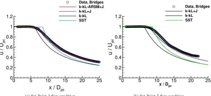
The jet core length and rate of decay are better predicted when using the k-kL+J model, as shown in figure 3(a) for Set Point 3. In particular, the jet core length is in better agreement with the experiment than the much longer core predicted using the SST turbulence model. Similarly, in figure 3(b) for Set Point 7, the k-kL+J model produces the best results as compared with experimental data and other turbulence models. Very good comparisons of the k-kL+J are shown in figure 4(a) for Set Point 3 and in figure 4(b) for

Set Point 7 for the velocity variations with radial direction at differentx/Djetlocations.

x / D

_jet

u

/

U

je t 0 5 10 15 20 25 0 0.2 0.4 0.6 0.8 1 1.2 Data, Bridges k-kL-ARSM+J k-kL+J k-kL SST

(a) Set Point 3 flow condition.

x / Djet

u

/

U

je t 0 5 10 15 20 25 0 0.2 0.4 0.6 0.8 1 1.2 Data, Bridges k-kL+J k-kL SST

(b) Set Point 7 flow condition.

Figure 3. Streamwise centerline velocity profiles using different linear RANS turbulence models. Symbols, Data-Bridges [18]; lines, FUN3D.

u / U

_jet

y /

D

jet 0 0.2 0.4 0.6 0.8 1 1.2 0 0.5 1 1.5 x/Djet = 2 x/Djet = 5

x/Djet = 10 Data, Bridges

x/Djet = 15

x/Djet = 20

FUN3D

(a) Set Point 3 flow condition.

u / U

_jet

y /

D

jet 0 0.2 0.4 0.6 0.8 1 1.2 0 0.5 1 1.5 x/Djet = 2 x/Djet = 5

x/Djet = 10 Data, Bridges

x/D_jet = 15 x/D_jet = 20 FUN3D

(b) Set Point 7 flow condition.

Figure 4. Velocity variations with radial direction at different x/Djet locations using k-kL+J turbulence model. Symbols, Data-Bridges [18]; lines, FUN3D.

The jet core length and rate of decay are very similar when using either k-kL-ARSM or k-kL+J turbulence models as shown in figure 5(a). Slight differences are observed between these models in predicting turbulent kinetic energy as shown in figure 5(b). This verifies that the ARSM is almost inactive away from walls. This results from using the blending function f2 (eqs. 22 and 23) to switch between linear and nonlinear production.

(a) Streamwise centerline velocity. (b) Streamwise centerline turbulence kinetic energy. Figure 5. Comparison between linear and nonlinear k-kL turbulence models. Symbols, Set Point 3 Data-Bridges [18]; lines, FUN3D.

4.2

High-Speed Mixing Layer

In this case, subsonic and supersonic streams, initially separated by a splitter plate, come into contact and form a shear layer. Results are compared with test case 4 in the experiment of Goebel and Dutton [19]. At the entrance of the mixing layer, the flow conditions are M1 = 2.34, Tt1 = 360 K, and U1 = 616 m/s for the high-speed stream and M2 = 0.3, Tt2 = 360 K, and U2 = 100 m/s for the low-speed stream. For this case, the convective Mach number, Mc, is 0.86. For Mc >0.5, the flow is considered compressible, and compressibility correction through the use of +J correction is expected to improve the prediction. Figure 6 shows the flow setup for the high-speed mixing layer case. Figure 7 shows the effect of using +J correction in the prediction of the high-speed mixing layer at x = 100 mm. The raw data of the velocity correctly matches the experimental data using +J correction as shown in figure 7(a). The shear stress profile and peak value are in very good agreement using +J correction with experimental data as shown in figure 7(b).

We have used k-kL+J, k-kL-ARSM+J, SST, and LES [35] turbulence models and compared the results with the experimental data as shown in figures 8, 9, and 10. Figure 8(a) shows the raw data comparisons between the three turbulence models and experimental data for the raw velocity profile at x = 100 mm downstream of the splitter plate. Both k-kL turbulence models show good results when compared with the other models. The LES results were offset from the other turbulence model results and experimental data. As the mixing layer flow developed, a self-similar flow profile could be used to report the results. Using this approach, we plotted the velocity normalized values, un _{versus the normalized distance y}n _{instead of the} raw data: yn= y−y0.5 b and u n₌ U−U2 ∆U , (26) b=y0.9−y0.1and∆U =U1−U2 (27) yrat un =r (28)

Figure 8(b) shows the comparisons between the three turbulence models, normalized results and experimental data. The results are similar using this approach. However, the SST results were still missing the data at

Figure 6. Mixing layer case 4, Mc = 0.86. U (m/s) y ( m m ) 0 100 200 300 400 500 600 700 -20 -15 -10 -5 0 5 10 15 20 exp, x=100 (mm)_k-kL k-kL+J

(a) Raw velocity results.

-u‘v‘ (m2/s) y ( m m ) 0 1000 2000 3000 4000 -20 -15 -10 -5 0 5 10 15 20 exp, x = 100 (mm) k-kL k-kL+J

(b) Raw shear stress results.

Figure 7. 2D Mixing Layer: Effect of +J correction in the prediction of the high-speed mixing layer at x = 100mm.

the edge of the mixing layer. Figure 9(a) shows the data comparisons between the three turbulence models and experimental data for the raw shear stress at x = 100 mm downstream of the splitter plate. Both k-kL turbulence models show good results when compared with the data from the other models. The shear stress results from the k-kL and LES turbulence models are comparable with the experimental data. The LES results were again offset from the other turbulence model results and experimental data. Now, we normalize

U (m/s) y ( m m ) 0 100 200 300 400 500 600 700 -20 -15 -10 -5 0 5 10 15 20 exp, x=100 (mm)_k-kL-ARSM+J k-kL+J SST LES

(a) Raw results.

(U-U2)/ U (y -y 0 .5 )/ b 0 0.2 0.4 0.6 0.8 1 1.2 -1 -0.5 0 0.5 1 exp, x = 100 {mm} k-kL-ARMS+J k-kL+J SST LES (b) Normalized results.

Figure 8. 2D Mixing Layer: Comparison of turbulence model velocity results at x = 100 mm.

the shear stress by the square of the velocity difference as:

−u0_v0 ∆U2

Figure 9(b) shows the normalized results. It is clear that the LES and k-kL produced better results compared with experimental data than results from the SST turbulence model.

-u‘v‘ (m2/s) y ( m m ) 0 1000 2000 3000 -20 -15 -10 -5 0 5 10 15 20 exp, x=100 mm k-kL-ARSM+J k-kL+J SST LES

(a) Raw results.

-u‘v‘ / U2 (y y0 ) /b 0 0.005 0.01 0.015 -1.5 -1 -0.5 0 0.5 1 1.5 exp, x=100 mm k-kL-ARSM+J k-kL+J SST LES (b) Normalized results.

Figure 9. 2D Mixing Layer: Comparison of turbulence model shear stress results at x=100 mm. Figure 10 shows the change of shear layer thickness, b, with distance, x, from the end of the splitter plate comparisons with experimental data. The medium and fine grid results are very similar indicating grid

convergence as shown in figure 10(a). The k-kL turbulence models are comparable with the LES results and are closer to the experimental data when compared with SST results as shown in figure 10(b).

In general, all of the turbulence models examined appear to predict the streamwise velocity profiles, and it appears that the k-kL is much better than the two-equation SST model. Overall, they are closer to the experimental values in predicting the turbulence intensity, turbulent shear stress, and shear layer thickness. The results using the k-kL are in very good agreement with experimental and LES data.

x (mm) b ( m m ) 50 100 150 2 4 6 8 10 12 14 16 18 20 Case4 Data k-kL+J Fine Grid k-kL+J Medium Grid k-kL+J Coarse Grid

(a) Grid sensitivity.

x (mm) b ( m m ) 50 100 150 2 4 6 8 10 12 14 16 18 20 Case4 Data k-kL+J Medium SST Medium LES

(b) Turbulence models comparisons. Figure 10. Shear layer thickness comparisons for different turbulence models.

4.3

2D NASA Subsonic Wall-Mounted Hump

Figure 11 shows a sketch of the 2D NASA wall-mounted hump test case with boundary conditions used in this analysis. The model is mounted between two glass endplate frames, and both leading and trailing

edges are faired smoothly with a wind tunnel splitter plate [20]. This is a nominally two-dimensional experiment, treated as such for the CFD validation. The primary focus of this case is to assess the ability of turbulence models to predict 2D separation from a smooth body (caused by adverse pressure gradient) as well as subsequent reattachment and boundary layer recovery. Since its introduction, this particular case has proved to be a challenge for all known RANS models. Models tend to underpredict the turbulent shear stress in the separated shear layer, and therefore, tend to predict too long a separation bubble. For this case, the reference freestream velocity is approximately 34.6 m/s (M = 0.1). The back pressure is chosen to achieve the desired flow. The upstream “run” length is chosen to allow the fully turbulent boundary layer to develop naturally, and achieve approximately the correct boundary layer thickness upstream of the hump. The upper boundary is modeled in the CFD as an inviscid (slip) wall, and it includes a contour to its shape to approximately account for the blockage caused by the end plates in the experiment. The grid size is 91,718 nodes with hex cells. Menter et al. [3–5] noticed that the kL-based turbulence models produce under- and over-shoot of the skin friction in the separated flow region as shown in figure 12(a) usingC13= 1.0 from equation 11. This is the only quantity that shows such behaviour. To reduce these jumps in skin friction, a C13 value of 0.5 is selected for the linear k-kL two-equation turbulence model. For ARSM, we used a value of 0.25. C13 has very minimal effect in other quantities as shown for shear stress at x/c = 1.1 (see figure 12(b)).

x/c

C

f -0.5 0 0.5 1 1.5 2 -0.004 -0.002 0 0.002 0.004 0.006 0.008 exp k-kL, C_l3=0.25 k-kL, C_l3=0.50 k-kL, Cl3=1.00

(a) Skin friction results.

u’v’/Uinf2 y /c -0.030 -0.025 -0.02 -0.015 -0.01 -0.005 0 0.05 0.1 0.15 0.2 exp x/c=1.1 k-kL, C_l3=0.25 k-kL, C_l3=0.0 k-kL, C_l3=1.0

(b) Shear stress results. Figure 12. Wall-Mounted Hump: calibration of k-kL turbulence model.

This case is used to calibrate ARSM to optimize the results. The basic ARSM completely missed the separation and reattachment locations as shown in figure 13(a). Adjustinga2 to 0.8 from 0.7 and limiting thekLproduction (PkL) as shown in equation 18 significantly improves the results of ARSM. LimitingPkL allows the RANS model to overcome the deficit in predicting shear stress level as shown in figure 13(b). This combination produces the best results for skin friction and other flow quantities such as velocity and shear stress. Figure 14 shows the comparisons between two-equation turbulence models and experimental data. The ARSM gives the best skin friction results as compared with other models and experimental data. All kL formulations missed the peak in Cf near x/c = 0.4. SST is the only model that predicted the skin friction peak. However, SST completely missed the shear stress peak and yielded a separation bubble size similar to k-kL-QCR and k-kL. All kL formulations improve the prediction of the shear stress peak with the best results generated using the k-kL-ARSM.

Figure 15 shows comparisons of two-equation turbulence models, production to dissipation ratio (P/) results at different x/c locations. Two locations are chosen in the separated flow region (x/c = 0.8 and 0.9). x/c = 1.1 is where the experimental data is reattached, and x/c = 1.3 is where the turbulence model data

x/c

C

f -0.5 0 0.5 1 1.5 2 -0.004 -0.002 0 0.002 0.004 0.006 0.008 exp ARSM+Prod+a₂ ARSM+a₂ ARSM

(a) Skin friction results.

u’ v’ /Uinf2 y /c -0.030 -0.025 -0.02 -0.015 -0.01 -0.005 0 0.05 0.1 0.15 0.2 exp x/c=1.1 ARSM+Prod+a₂ ARSM+Prod ARSM

(b) Shear stress results. Figure 13. Wall-Mounted Hump: Calibration of k-kL+ARSM turbulence model.

x/c Cf -0.5 0 0.5 1 1.5 2 -0.004 -0.002 0 0.002 0.004 0.006 0.008 exp k-kL-ARSM k-kL-QCR k-kL SST

(a) Skin friction results.

u’ v’ /Uinf2 y /c -0.030 -0.025 -0.02 -0.015 -0.01 -0.005 0 0.05 0.1 0.15 0.2 exp x/c=1.1 k-kL-ARSM k-kL-QCR k-kL SST

(b) Shear stress results.

Figure 14. Wall-Mounted Hump: Skin friction and shear stress results using two-equation turbulence models.

show the flow is fully attached. At x/c = 0.8, the k-kL-ARSM generates more than double P/produced by all the other models. It does still have a larger value at x/c = 0.9. For the attachment locations, all the kL models generate a similar level of P/ which is higher than the SST level. In the separated flow regions, it is believed that the mechanism that generates the high shear stress is driven by high production dissipation ratio.

Table 3 reports separation and reattachment locations, bubble size and % error results from different turbulence models. The experimental data bubble size was 0.435c. The k-kL, SST and k-kL-QCR have a larger bubble size than experimental data with 33.7, 41.6, and 43.2% error, respectively. Out of all the two-equation turbulence models, k-kL-ARSM produces a bubble size that is close to the experimental data

(a) x/c=0.8. (b) x/c=0.9.

(c) x/c=1.1. (d) x/c=1.3.

Figure 15. Wall-Mounted Hump: Comparison of two-equation turbulence model production/dissipation results.

with 3.4% error. However, only k-kL-ARSM closely predicts the reattachment location around x/c = 1.1. As a result, this model has the smallest % error. From the results presented in this section, it is clear that k-kL-ARSM produces the best results from all the kL formulations.

4.4

Transonic Bump

This shock-induced separation case at transonic speed adds complexity to modeling separated flow. Also, axisymmetry removes the difficulty experienced when conducting the experiment than for the two-dimensional flow experiment. Figure 16 shows a sketch of the axisymmetric transonic bump case with boundary conditions used in this analysis. This is a transonic, M∞= 0.875 case at Re = 2.763 million based on L = chord length. The purpose here is to provide a validation case that establishes the model’s ability

Table 3. Wall-Mounted Hump: Separation and reattachment locations.

Results Separation Reattachment Bubble Size % Error x/c location x/c location (c) Experimental data 0.665 1.100 0.435 — SST 0.654 1.270 0.616 41.6 k-kL 0.658 1.240 0.582 33.7 k-kL-QCR 0.657 1.280 0.623 43.2 k-kL-ARSM 0.660 1.110 0.450 3.4

to predict separated flow. For this particular axisymmetric transonic bump case, the experimental data are from Bachalo and Johnson [21]. The experiment utilized a cylinder of 0.152 m diameter in a closed return, variable density, and continuous running tunnel with 21% open porous-slotted upper and lower walls. The boundary layer incident on the bump was approximately 1 cm thick. The bump chord was 0.2032 m. In the experimental case, with a freestream Mach number of 0.875, the shock and trailing-edge adverse pressure gradient results in flow separation with subsequent reattachment downstream.

Figure 16. Transonic Bump and boundary conditions.

The majority of RANS turbulence models fail to predict the correct reattachment of this separated flow case, with the separation bubble size overpredicted by up to 23.7% as reported in Table 4 using SST. The k-kL cuts the error by more than 40%. The k-kL-QCR slightly improves the results to 18.75%, whereas the k-kL-ARSM stayed closer to the k-kL at 13%. The most improvement results from using the k-kL model. Figure 17(a) shows surface pressure comparisons between two-equation kL and SST turbulence models with experimental data [21]. SST predicts a further upstream location of the shock at x/c = 0.65 compared with experimental data at 0.66, but it produces the best profile in the x/c region of 0.8 through 1.2. Figure 17(b)

Table 4. Transonic Bump: Separation and reattachment locations.

Results Separation Reattachment Bubble Size % Error x/c location x/c location (c) Experimental data 0.700 1.100 0.400 — SST 0.665 1.160 0.495 23.7 k-kL 0.669 1.120 0.451 12.7 k-kL-QCR 0.665 1.140 0.475 18.75 k-kL-ARSM 0.701 1.050 0.349 13.0

shows typical velocity contours from most two-equation turbulence models. Next, we evaluate the capabilities

x/c

c

p 0.4 0.6 0.8 1 1.2 1.4 1.6 1.8 -1 -0.8 -0.6 -0.4 -0.2 0 0.2 exp k-kL-QCR k-kL-ARSM k-kL SST

(a) Surface pressure. (b) Typical velocity contours.

Figure 17. Axisymmetric Transonic Bump: Comparison of two-equation turbulence model results. of these models in predicting shear stress magnitudes. Figure 18 shows that k-kL-ARSM improves the result at x/c = 0.813. However, there are no improvements from any of the models at x/c = 1.375. For the velocity results, k-kL-ARSM improves the results at x/c = 1.375 and shows notable improvements at x/c = 0.813, as shown in figure 19.

4.5

Supersonic Compression Corner

This case examines supersonic flow over an axisymmetric compression corner. Experimental data are documented in references 22 and 34. Figure 20 shows the supersonic compression corner experimental configuration. The model is a 5.08 cm diameter cylinder with a 30-degree flare, which generates a shock wave. The cylinder has an upstream cusped nose designed to minimize the strength of the shocks, and data indicates that reflected shocks from the tunnel walls have no effect in the measurement region of interest. The flare is located x/c = 1.0 m downstream of the cusp-tip, allowing a turbulent boundary layer to develop upstream of the shock-wave boundary-layer interaction. The flare surface begins at x = 0.0 cm and ends at x = 5.196 cm. The test section has a Mach number of 2.85, a unit Reynolds number of 16x106/m, a stagnation pressure of 1.7 atm, and a stagnation temperature of 270 K. Figure 21(a) shows normalized pressure comparisons between two-equation kL and SST turbulence models with experimental data [21]. SST predicts the earlier location of the separation at x = -3.82 cm compared with experimental data at -2.73 cm, but it produces the best pressure recovery profile in the 0 cm<x<5 cm region. Figure 21(b) shows typical

u‘ v‘ /U2 inf y /c -0.020 -0.015 -0.01 -0.005 0 0.02 0.04 0.06 0.08 0.1 exp, x/c = 0.813 k-kL-QCR k-kL-ARSM k-kL SST (a) x/c=0.813. u‘ v‘ /U2 inf y /c -0.020 -0.015 -0.01 -0.005 0 0.02 0.04 0.06 0.08 0.1 exp, x/c = 1.375 k-kL-QCR k-kL-ARSM k-kL SST (b) x/c=1.375.

Figure 18. Axisymmetric Transonic Bump: Comparison of two-equation turbulence model shear stress results. u/Uinf y /c -0.5 0 0.5 1 1.5 0 0.02 0.04 0.06 0.08 0.1 0.12 0.14 exp, x/c = 0.813 k-kL-QCR k-kL-ARSM k-kL SST (a) x/c=0.813. u/Uinf y /c -0.5 0 0.5 1 1.5 0 0.02 0.04 0.06 0.08 0.1 0.12 0.14 exp, x/c = 1.375 k-kL-QCR k-kL-ARSM k-kL SST (b) x/c=1.375.

Figure 19. Axisymmetric Transonic Bump: Comparison of two-equation turbulence model velocity results.

Mach contour from a two-equation turbulence model. Table 5 reports the results of separation, reattachment, and bubble size using different turbulence models and experimental data. The k-kL and k-kL-ARSM produce the closest separation and reattachment locations compared with experimental data. SST shows the largest error of 60% in bubble size compared with k-kL-ARSM of 2%. The separation location is closely computed using k-kL-ARSM at x = -2.75 cm followed by k-kL at -2.81 cm. Both SST and k-kL-QCR produced the farthest separation locations at -3.82 cm and -3.41 cm, respectively. Similarly, the reattachment location is better computed using k-kL-ARSM. In general, the overall best results were produced using k-kL-ARSM.

Figure 20. Supersonic Compression Corner Experimental Configuration [22].

x (cm)

p

/p

0 -6 -4 -2 0 2 4 6 8 0 0.05 0.1 0.15 0.2 Experiment k-kL-QCR k-kL-ARSM k-kL SST

(a) Normalized pressure. (b) Mach contour using k-kL-ARSM.

Figure 21. Supersonic Compression Corner: comparison of kL-based turbulence model, SST and experimen-tal data.

separation region and x = 1.732 cm in the reattachment region. Figure 22 shows that k-kL-ARSM improves the result at the location in the separation region. However, there are no significant improvements from any of the models in the reattachment region.

5

Concluding Remarks

With the exception of Reynolds stress models, the turbulent kinetic energy is exclusively used as one of the transport equations in multi-equation turbulence models. The foundation of this equation is well established and accepted. The scale-determining equation, though, is considered the weakest link, even when full Reynolds stress and hybrid RANS/LES formulations are considered. The most important difference is that the kL formulation leads to a natural inclusion of higher order velocity derivatives into the source terms of the scale equation.

The present report documents the development of kL-based linear and nonlinear turbulence models. A systematic investigation was conducted to assess the implementation of these models in the FUN3D CFD code utilizing several aerodynamic configurations. The computed results were compared with available experimental data and the SST turbulence model. This investigation provided significant insight into the applications and capabilities of turbulence models in the prediction of attached, separated, and corner flows. The jet correction improves the results of k-kL for jet and free shear flow cases. Blending function is used to eliminate the effect of these corrections for near wall flows. These corrections do not alter any of the other results of the cases presented in this report. In a high-speed mixing layer, the spreading rates for k-kL+J are

Table 5. Supersonic Compression Corner: Separation and reattachment locations.

Results Separation Reattachment Bubble Size % Error x location (cm) x location (cm) (cm) Experimental data -2.73 0.97 3.70 — SST -3.82 2.10 5.92 60.0 k-kL -2.81 1.34 4.15 12.1 k-kL-QCR -3.41 1.65 5.06 36.7 k-kL-ARSM -2.75 0.88 3.63 2.0 u₀ y ( c m ) -0.2 0 0.2 0.4 0.6 0.8 1 0 0.5 1 1.5 2 2.5 exp, x=-2.0 (cm) k-kL-QCR k-kL-ARSM k-kL SST (a) x = -2.0 cm. u₀ y ( c m ) -0.2 0 0.2 0.4 0.6 0.8 1 0 0.5 1 1.5 2 2.5 exp, x=1.732 (cm) k-kL-QCR k-kL-ARSM k-kL SST (b) x = 1.732 cm.

Figure 22. Supersonic Compression Corner: comparisons of kL-based turbulence models, SST and experi-mental data.

comparable with experimental data and much better than the results produced by SST turbulence models. The wall-mounted hump geometry presents subsonic separated flow over a smooth body. This is a simple geometry and a challenging problem for RANS eddy viscosity-based turbulence models. Typical RANS model results have more than a 40% error predicting the separation bubble. These also underpredict maximum shear stress by 50%. Linear k-kL reduces the error down to 33.7%. The nonlinear k-kL-QCR did not improve any of these predictions. However, the k-kL-ARSM eliminated most of the error and significantly improve the level of shear stress to be much closer to experimental data.

The axisymmetric transonic bump and compression corner geometries represent the next level of a flow complexity because these cases contain separated flow regions that interact with a shock. The transonic case of Mach 0.875 is a complex flow that proves to be challenging to most RANS turbulence models. The improvements using k-kL-ARSM is quite good.

A supersonic flow of Mach 2.85 over a cylinder with a 30-degree flare was computed and compared with the experimental data. For this case, good agreement was obtained in predicting the surface pressure and the size of the separation bubble using kL-based turbulence models. The error in computing the size was under 13%. The SST overpredicted the bubble size by 60%.

In general, the k-kL-ARSM gives better agreement with experimental data than the other kL formulations and SST models for all the cases presented in this report.

References

[1] B. E. Launder and D. B. Spalding. Lectures in mathematical models of turbulence. Academic Press, London, 1972.

[2] J. Rotta. Statistische theorie nichthomogener turbulenz. Zeitschrift f¨ur Physik, 129(6):547–572, 1951. [3] F. R. Menter, Y. Egorov, and D. Rusch. Steady and Unsteady Flow Modeling Using the k-√kL model. In

K. Hanjali`c, Y. Nagano, and S. Jakirlic, editors,Turbulence, Heat and Mass Transfer, 5th International symposium, Proceedings, pages 403–406, Dubrovnik, Croatia, 2006.

[4] F.R. Menter and Y. Egorov. The scale-adaptive simulation method for unsteady turbulent flow pre-dictions. part 1: Theory and model description. Flow, Turbulence and Combustion, 85(1):113–138, 2010.

[5] Y. Egorov, F.R. Menter, R. Lechner, and D. Cokljat. The scale-adaptive simulation method for unsteady turbulent flow predictions. part 2: Application to complex flows. Flow, Turbulence and Combustion, 85(1):139–165, 2010.

[6] F. R. Menter. Improved Two-Equation k-ω Turbulence Models for Aerodynamic Flows. NASA TM-103975, Oct. 1992.

[7] K. S. Abdol-Hamid. Assessments of k-kl Turbulence Model Based on Menter’s Modification to Rotta’s Two-Equation Model. International Journal of Aerospace Engineering, 2015:1–18, 2015.

[8] K. S. Abdol-Hamid, S. P. Pao, C. Hunter, K. Deere, S. Massey, and A. Elmiligui. PAB3D: It’s History in the Use of Turbulence Models in the Simulation of Jet and Nozzle Flows. AIAA Paper 2006-0489, Jan. 2006.

[9] K. S. Abdol-Hamid, Jan-Rene`e Carlson, and Christopher L. Rumsey. Verification and Validation of the k-kL Turbulence Model in FUN3D and CFL3D Codes. AIAA Paper 2016-3941, Jun. 2016.

[10] http://turbmodels.larc.nasa.gov. Accessed: 2015-09-01.

[11] C.R. Rumsey, B.R. Smith, and G.P. Huang. Description of a Website Resource for Turbulence Model Verification and Validation. AIAA Paper 2010-4742, June 2010.

[12] B.E. Launder, G.J. Reece, and W. Rodi. Progress in the development of a Reynolds stress turbulence closure. J. Fluid Mech., 68:537–566, 1975.

[13] C. G. Speziale, S. Sarkar, and T. B. Gatski. Modeling the pressure-strain correlation of turbulence: an invariant dynamical systems approach. J. Fluid Mech., 227:245–272, 1991.

[14] K. Hanjalic. Closure Models for Incompressible Turbulent Flows. Von Krmn Institute, 2004.

[15] C.L. Rumsey and T.B. Gatski. Summary of EASM Turbulence Models in CFL3D With Validation Test Cases. NASA TM–2003-212431, June 2003.

[16] S.S. Girimaji. Fully Explicit and Self-Consistent Algebraic Reynolds Stress Model. Theoret. Comp. Fluid Dynamics, 8:387–402, 1996.

[17] P.R. Spalart. Strategies for Turbulence Modelling and Simulation,. International Journal of Heat and Fluid Flow, 21:252–263, 2000.

[18] J. Bridges and C. Brown. Parametic Testing of Chevrons on Single Flow Hot Jets. AIAA Paper 2004-2824, 2004.

[19] S. G. Goebel and J. C. Dutton. Experimental Study of Compressible Turbulent Mixing Layers. AIAA Journal, 29(4):538–546, 1991.

[20] D. Greenblatt J. W. Naughton, S. A. Viken. Skin-Friction Measurements on the NASA Hump Model. AIAA Journal, 44(6):1255–1265, 2006.

[21] W. D. Bachalo and D. A. Johnson. Transonic, turbulent boundary-layer separation generated on an axisymmetric flow model. AIAA Journal, 24(3):437–443, 1986.

[22] J. L. Brown S. E. Dunagan and J. B. Miles. Interferometric Data for a Shock/Wave Boundary-Layer Interaction. NASA TM–1986-88227, 1986.

[23] P. L. Roe. Approximate Riemann Solvers, Parameter Vectors, and Difference Schemes. J. Comp. Phys., 43:357–372, 1981.

[24] P. Batten, N. Clarke, C. Lambert, and D.M. Causon. On the Choice of Wavespeeds for the HLLC Riemann Solver. SIAM J. Sci. Comput., 18:1553–1570, 1997.

[25] M. Sun and K. Takayama. Artificially Upwind Flux Vector Splitting Scheme for the Euler Equations. J. Comp. Phys., 189:305–329, 2003.

1996-1704, May 1996.

[27] B. van Leer. Towards the Ultimate Conservative Difference Schemes V. A second order sequel to Godunov’s Method. J. Comp. Phys., 32:101–136, 1979.

[28] P. L. Roe. Characteristic-Based Schemes for the Euler Equations. Annual Review of Fluid Mechanics, 18:337–365, 1986.

[29] T.J. Barth and D.C. Jespersen. The Design and Application of Upwind Schemes on Unstructured Meshes. AIAA Paper 1989-0366, Jan. 1989.

[30] V. Venkatakrishnan. Convergence to Steady State Solutions of the Euler Equations on Unstructured Grids with Limiters. J. Comp. Phys., 118:120–130, 1995.

[31] W.K. Anderson and D.L. Bonhaus. An Implicit Upwind Algorithm for Computing Turbulent Flows on Unstructured Grids. Computers and Fluids, 23(1):1–22, 1994.

[32] W.K. Anderson, R.D. Rausch, and D. L. Bonhaus. Implicit/Multigrid Algorithms for Incompressible Turbulent Flows on Unstructured Grids. J. Comp. Phys, 128:391–408, 1996.

[33] S. Wallin and A. V. Johansson. An Explicit Algebraic Reynolds Stress Model for Incompressible and Compressible Turbulent Flows. Journal of Fluid Mechanics, 403:89–132, 2000.

[34] J. Miles J. Wideman, J. Brown and O. Ozcan. Surface Documantation of a 3-D Supersonic, Shock Wave/Boundary Interaction. NASA TM–1994-108824, 1994.

[35] J. R. DeBonis M. R. Mankbadi and N. J. Georgiadis. Large-Eddy Simulation of a Compressible Mixing Layer and the Significance of Inflow Turbulence. AIAA Paper 2017-0316, Jan. 2017.