UCLA
UCLA Electronic Theses and Dissertations
Title
From Fully-Supervised, Single-Task to Scarcely-Supervised, Multi-Task Deep Learning for Medical Image Analysis
Permalink https://escholarship.org/uc/item/9366k4tv Author Imran, Abdullah-Al-Zubaer Publication Date 2020 Peer reviewed|Thesis/dissertation
UNIVERSITY OF CALIFORNIA Los Angeles
From Fully-Supervised, Single-Task to Scarcely-Supervised, Multi-Task Deep Learning for Medical Image Analysis
A dissertation submitted in partial satisfaction of the requirements for the degree Doctor of Philosophy in Computer Science
by
Abdullah-Al-Zubaer Imran
c
Copyright by Abdullah-Al-Zubaer Imran
ABSTRACT OF THE DISSERTATION
From Fully-Supervised, Single-Task to Scarcely-Supervised, Multi-Task Deep Learning for Medical Image Analysis
by
Abdullah-Al-Zubaer Imran
Doctor of Philosophy in Computer Science University of California, Los Angeles, 2020
Professor Demetri Terzopoulos, Chair
Image analysis based on machine learning has gained prominence with the advent of deep learning, particularly in medical imaging. To be effective in addressing challenging image analysis tasks, however, conventional deep neural networks require large corpora of annotated training data, which are unfortunately scarce in the medical domain, thus often rendering fully-supervised learning strategies ineffective.
This thesis devises for use in a variety of medical image analysis applications a series of novel deep learning methods, ranging from fully-supervised, single-task learning to scarcely-supervised, multi-task learning that makes efficient use of annotated training data. Specifically, its main contributions include (1) fully-supervised, single-task learning for the segmentation of pulmonary lobes from chest CT scans and the analysis of scoliosis from spine X-ray images; (2) supervised, single-task, domain-generalized pulmonary segmentation in chest X-ray images and retinal vasculature segmentation in fundoscopic images; (3) largely-unsupervised, multiple-task learning via deep generative modeling for the joint synthesis and classification of medical image data; and (4) partly-supervised, multiple-task learning for the combined segmentation and classification of chest and spine X-ray images.
The dissertation of Abdullah-Al-Zubaer Imran is approved. Guy Van den Broeck
Kai-Wei Chang Song-Chun Zhu
Demetri Terzopoulos, Committee Chair
University of California, Los Angeles 2020
TABLE OF CONTENTS
1 Introduction . . . 1
1.1 The Problem of Limited Training Data . . . 1
1.2 Generative Models . . . 2
1.3 Semi-Supervised Learning . . . 4
1.4 Contributions . . . 5
1.5 Overview. . . 8
2 Related Work . . . 10
2.1 Supervised Learning for Medical Image Segmentation . . . 10
2.1.1 3D Segmentation . . . 12
2.1.2 2D Segmentation . . . 18
2.2 Limited Supervision. . . 20
2.2.1 Semi-Supervised Learning . . . 21
2.2.2 Deep Generative Modeling . . . 22
2.2.3 Domain Generalization . . . 25
2.2.4 Multitask Learning . . . 26
3 Models and Associated Learning Algorithms . . . 28
3.1 Fully-Supervised Learning Models . . . 28
3.1.1 3D Pulmonary Segmentation in Chest CT Images . . . 28
3.1.2 Segmentation and Scoliosis Quantification in Spine Radiographs . 30 3.2 Learning From Limited Labeled Data . . . 33
3.2.1 Simultaneous Image Generation and Classification . . . 34
3.2.3 Semi-Supervised Multitask Learning . . . 48
3.2.4 Self-Supervised, Semi-Supervised, Multi-Task Learning . . . 52
4 Experimental Evaluations . . . 59
4.1 3D Segmentation of Pulmonary Lobes. . . 59
4.1.1 Implementation Details . . . 59 4.1.2 LIDC Results . . . 60 4.1.3 LTRC Results . . . 62 4.1.4 LOLA11 Results . . . 63 4.1.5 Robustness Analysis . . . 64 4.1.6 Speed Analysis . . . 65
4.2 2D Segmentation & Analysis of Scoliosis . . . 66
4.2.1 Implementation Details . . . 66
4.2.2 Segmentation Results . . . 67
4.2.3 Scoliosis Results. . . 68
4.3 Semi-Supervised Simultaneous Image Generation and Classification . . . 69
4.3.1 Implementation Details . . . 69
4.3.2 Evaluation . . . 72
4.3.3 Results. . . 74
4.4 Domain Generalization Without Domain-Specific Data . . . 83
4.4.1 Implementation Details . . . 83
4.4.2 Results. . . 84
4.5 Semi-Supervised Multi-Task Learning . . . 89
4.5.1 Implementation Details . . . 90
4.5.3 Segmentation and Classification . . . 95
4.6 Self-Supervised Semi-Supervised Multi-Task Learning . . . 97
4.6.1 Implementation Details . . . 97
4.6.2 Classification Results . . . 99
4.6.3 Segmentation Results . . . 100
4.6.4 Statistical Analysis . . . 103
5 Conclusions and Future Research Directions . . . 108
A Datasets . . . 111
LIST OF FIGURES
1.1 Disparities in the distributions of different datasets . . . 2
1.2 Discriminative vs generative models . . . 3
1.3 Spectrum of thesis contributions. . . 5
2.1 An axial lung CT slice with visible fissures . . . 13
2.2 Challenges in segmenting lung lobes . . . 14
2.3 Illustration of the calculation of Cobb angle . . . 19
2.4 Generated images by VAEs and GANs . . . 23
3.1 PDV-Net model for the segmentation of lung lobes . . . 29
3.2 Progressive U-Net Architecture . . . 30
3.3 Architectural distinction of VAE, GAN, VAE-GAN, and MAVEN . . . 34
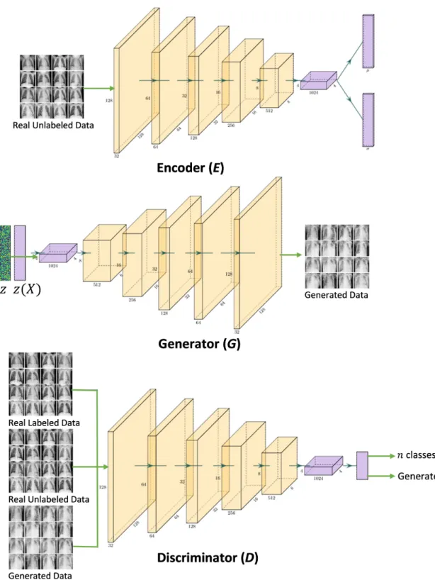
3.4 The three convolutional neural networks, E, G, and D, in the MAVEN. . . . 36
3.5 Schematic of the PASS model . . . 41
3.6 APPAU-Net model . . . 48
3.7 Pyramid progressive attention U-Net architecture . . . 49
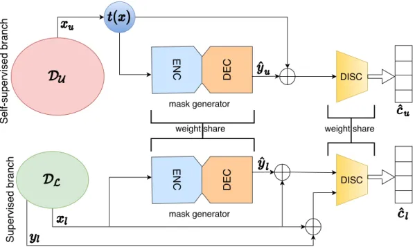
3.8 Schematic of the S4MTL model . . . 53
3.9 Detailed architecture of the segmentation mask generator (G) network. . . . 54
4.1 Qualitative comparison of PDV-Net against U-Net and DV-Net . . . 61
4.2 Bland-Altman agreements of PDV-Net with ground truth. . . 62
4.3 Sagittal visualization of LOLA11 segmentation by PDV-Net . . . 64
4.4 Lobe-wise and overall Dice scores vs emphysema indices of LTRC cases . . . 65
4.5 Boundary visualization of the predicted vertebrae masks . . . 68
4.7 Whisker-Box plots of all six models in segmenting 18 vertebrae . . . 70
4.8 Better agreement of our model over the baselines with GT . . . 70
4.9 Scoliosis measurement through the segmentation of vertebrae . . . 71
4.10 Visual comparison of image samples from the SVHN dataset . . . 75
4.11 Histograms of the real SVHN and model-generated data . . . 76
4.12 Visual comparison of image samples from the CIFAR-10 dataset . . . 77
4.13 Histograms of the real CIFAR-10 and model-generated data . . . 79
4.14 Visual comparison of image samples from the CXR dataset . . . 80
4.15 Visual comparison of image samples from the SLC dataset . . . 82
4.16 Lung segmentation from a chest X-Ray image . . . 85
4.17 Retinal vessel segmentation from a fundus image . . . 85
4.18 Visualization of lung boundaries in an X-Ray from MCU . . . 87
4.19 Visualization of retinal vessel segmentation in STARE . . . 88
4.20 Visual comparison of the semi-supervised lung segmentation . . . 90
4.21 Loss plots for U-Net with varying losses on the MCU dataset . . . 91
4.22 Accuracy plots for U-Net with varying losses on the MCU dataset . . . 91
4.23 Visual comparison of the lung segmentation in an abnormal X-Ray . . . 95
4.24 Label distributions across the splits of the Spine and Chest datasets . . . 98
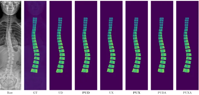
4.25 Consistent improvement in segmentation by S4MTL . . . . 100
4.26 Consistent improvement in classification by S4MTL . . . 100
4.27 Satisfactory balance between training and validation losses . . . 101
4.28 Spine Dataset: Boundary visualization of a predicted vertebra mask . . . 102
4.29 Chest Dataset: Boundary visualization of the predicted lung masks . . . 103
4.30 Bland-Altman plots showing good agreement for the S4MTL models . . . . . 105
A.1 LIDC CT data insights . . . 112
A.2 Example images of each class in SVHN . . . 115
A.3 Example images of each class in CIFAR-10 . . . 115
A.4 Examples images of each class in CXR . . . 116
A.5 Example images of each class in SLC . . . 116
A.6 Individual vertebra patch extraction . . . 117
A.7 Example images from the chest X-ray datasets . . . 118
LIST OF TABLES
3.1 Severity and treatment planning of scoliosis . . . 33
3.2 Architecture details of the shape encoder (E) . . . 44
3.3 Architecture details of the Discriminator (D). . . 45
3.4 Architecture details of the Discriminator (D2) . . . 45
3.5 Architecture details of the Discriminator (D4) . . . 46
3.6 Architecture details of the Discriminator (D8) . . . 46
4.1 Performance comparison of PDV-Net against U-Net and DV-Net models . . 61
4.2 Performance evaluation of PDV-Net on LOLA11 . . . 63
4.3 Performance comparison of the vertebrae segmentation models . . . 68
4.4 Cobb angle and scoliosis severity classification performance . . . 72
4.5 Minimum FID and DDD scores achieved by MAVENs and other models . . 74
4.6 Minimum FID and DDD scores achieved by MAVENs and other models . . 74
4.7 Average cross-validation accuracy and class-wise F1 scores for SVHN . . . . 78
4.8 Average cross-validation accuracy and class-wise F1 scores for CIFAR-10 . . 79
4.9 Average cross-validation accuracy and class-wise F1 scores for CXR . . . 79
4.10 Average cross-validation accuracy and class-wise F1 scores for SLC . . . 83
4.11 Dice score comparison for retinal vessel segmentation by PASS . . . 84
4.12 Dice score comparison for lung segmentation by PASS . . . 85
4.13 Comparison of HD for lung segmentation . . . 86
4.14 Comparison of SSIM for lung segmentation. . . 86
4.15 Comparison of SSIM for retinal vessel segmentation . . . 86
4.16 Comparison of HD for retinal vessel segmentation . . . 86
4.18 Evaluation of segmentation-only performance on CHN . . . 93
4.19 Evaluation of segmentation-only performance on JSRT . . . 94
4.20 Evaluation of segmentation-only performance on Chest . . . 96
4.21 Performance evaluation of the APPAU-Net model . . . 97
4.22 Classification performance comparison of S4MTL against the baselines . . . 101
4.23 Lung segmentation performance comparison of S4MTL against the baselines 104 4.24 Vertebrae segmentation performance comparison of S4MTL against the baselines106 A.1 Split of the chest X-ray datasets . . . 116
ACKNOWLEDGMENTS
First, I cannot thank Professor Demetri Terzopoulos enough for supporting me as my advisor throughout my PhD program. Long before coming to UCLA, I got to know about his revolutionary work on deformable models for image segmentation, particularly the snake model. While I was pursuing a master’s degree at Delaware State University in medical image analysis, I contacted him inquiring about a potential PhD position in his group. During my SPIE 2016 conference trip in California, I got a chance to meet him in person at UCLA and thereafter was determined to pursue my PhD under his supervision. Without his support and assistance, I would not be where I am today. Throughout my PhD studies, he provided his unconditional support whenever I needed it, be it research matters or academic issues. He gave me a clear research direction and often spent hours discussing the progress of my research, even within his extremely tight schedule. Without his guidance and support, this thesis would never have eventuated. I am and will always remain grateful to him.
I would like to express my appreciation to Professors Song-Chun Zhu, Guy Van den Broeck, and Kai-Wei Chang for serving on my thesis committee and offering me their kind advice to make my dissertation stronger. Thanks to my committee, I was able to build my knowledge and skills to make progress in my research and write this dissertation.
Furthermore, I would like to express my deep appreciation to previous advisors Professor David Pokrajac at Delaware State University and Professor Predrag Bakic at the University of Pennsylvania. I thank them immensely for all their valuable inputs to my career, especially for guiding me through an excellent medical imaging research setting. I would also like to express my gratitude to my bachelor thesis advisor, Professor Boshir Ahmed at the Rajshahi University of Engineering & Technology, for piquing my interest in image processing research.
Special thanks goes to my industry mentors and colleagues, Dr. Nima Tajbakhsh at VoxelCloud, Inc., Dr. Kunal Vaidya, Dr. Alvin Chen, and Dr. Ameet Jain at Philips Corporate Research, and Dr. Zhen Qian and Dr. Chao Huang at Tencent Medical AI, for
giving me the opportunity to engage in research activities in corporate settings.
I am grateful to all the coauthors of my publications related to this dissertation for their valuable contributions to my work.
I am very fortunate to have been surrounded by wonderful labmates in the UCLA Computer Graphics and Vision Laboratory who helped me progress through my PhD program. I would like to thank Dr. Tomer Weiss, Dr. Masaki Nakada, Dr. Tao Zhao, Dr. Garett Ridge, Dr. Arul Jeyraj, Mr. Ali Hatamizadeh, and Mr. Alan Litteneker.
During the first year of my PhD program, I was funded by a research assistantship made possible by an unrestricted gift from VoxelCloud, Inc., which I gratefully acknowledge and for which I thank Dr. Xiaowei Ding.
Lastly, I would like to thank my parents, Mozammel Biswas and Firoza Khatun, who raised me with unconditional love. Without their support I could not have achieved any-thing significant in my life, let alone come this far. I also thank my sister Shumaya Khatun, and my friends Al Arafat and Mijanur Rahman Sahed for continuously encouraging me in my work.
VITA
2012 B.S. Computer Science & Engineering
Rajshahi University of Engineering & Technology (RUET) Rajshahi, Bangladesh
2012–2013 Lecturer of Computer Science & Engineering Northern University
Dhaka, Bangladesh
2013–2014 Lecturer of Computer Science & Engineering Ahsanullah University of Science & Technology Dhaka, Bangladesh
2016 M.S. Computer Science
Delaware State University Dover, Delaware, USA
2017 Lecturer of Electrical & Computer Engineering North South University
Dhaka, Bangladesh 2017–2018 Research Assistant
Computer Graphics & Vision Laboratory University of California, Los Angeles Los Angeles, California, USA
2018–2020 Teaching Assistant
Computer Science Department University of California, Los Angeles Los Angeles, California, USA
2018 Research & Development Intern Philips Corporate Research Boston, Massachusetts, USA
2019 Research Intern
Tencent Medical AI
CHAPTER 1
Introduction
A general objective of medical image computing is to make predictions. In the machine learning approach, predictions are enabled based on models trained on collections of medical image data. In deep learning, which involves neural network models with numerous hidden layers, significant hierarchical relationships within the data can be discovered algorithmically, replacing the traditional laborious hand-crafting of image feature extractions. However, training deep neural networks usually requires copious data. Given set of properly annotated or labeled training data (input-output pairs), a supervised learning algorithm can learn the mapping from input to output. A well-trained supervised model can make predictions about previously unseen examples.
1.1
The Problem of Limited Training Data
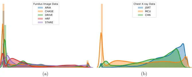
Although there has been explosive progress in the production of vast quantities of high resolution images, large collections of properly labeled or annotated images required for fully-supervised learning remain scarce. Expert annotation of medical images is expensive, time-consuming, and prone to human subjectivity, inconsistency, and error. Even when properly labeled datasets become available, they are often limited in size due to privacy issues and are highly imbalanced and non-uniformly distributed. In an imbalanced dataset, there will be an over-representation of common medical problems and an under-representation of rarer conditions. Such biases make the training of neural networks across multiple classes with consistent effectiveness very challenging.
Fundus Image Data ARIA CHASE DRIVE HRF STARE (a)
Chest X-ray Data JSRT MCU CHN
(b)
Figure 1.1: Disparities in the distributions of different datasets with varying data sources, sizes, ratios of normal/abnormal cases, etc.
independently and identically distributed (i.i.d.). However, this assumption may not hold in real world scenarios. Moreover, the problem is exacerbated due to varying medical conditions, imaging configurations and modalities, among other factors. Generalization refers to how well a model performs on previously unseen data. Difficulties further compound if the unseen data have different distributions than the training data (Figure1.1). This leads to the domain shift problem—when a model trained on data from one source does not generalize well to out of distribution (o.o.d.) test data from a different source, which can cause even the most sophisticated deep learning models to make non-intuitive, erroneous predictions.
1.2
Generative Models
The limited training data problem is traditionally mitigated through simplistic and often cumbersome data augmentation schemes, usually by creating new training examples through translation, rotation, flipping, etc. The missing or mismatched label problem may be addressed by evaluating similarity measures over the training examples; however, this is not always robust and its effectiveness depends largely on the performance of the similarity measuring algorithms. A more intuitive approach could be via generative modeling where the aforementioned issues are tackled algorithmically and automatically.
(a) Discriminative (b) Generative
Figure 1.2: Illustration of how a a generative model works compared to a discriminative model. The discriminative model learns only a decision boundary—a conditional distribution p(y|x)—whereas the generative model learns a joint probability distribution
p(x, y), thus enabling both generation and discrimination. (Images from
https://stanford.edu/~shervine/teaching/cs-229/cheatsheet-supervised-learning.) Unlike discriminative models that directly learn a classifier to make predictions given the training data, generative models learn the data generation process along with a classifier (Ng and Jordan, 2002). Figure 1.2 illustrates the working principle of a
generative model compared to a discriminative model. Generative models offer a powerful way to estimate data distributions through unsupervised learning, by constructing density over all the observable quantities (MacKay, 2003). This property of generative models is useful for unsupervised learning in realistic image generation and the clustering of images. Deep learning-based generative models work mostly based on latent coding, which helps elucidate hidden phenomena and similarities among observations. More generally, treating generative modeling as an auxiliary task leads to semantically meaningful, unsupervised representation learning. Furthermore, generative modeling can infer causal relations as opposed to mere data correlations (Rottman and Hastie,2014).
Our medical image analysis models are expected to learn from small quantities of labeled data, while also leveraging larger quantities of unlabeled examples, and to achieve effective generalization for consistent performance across different data domains. To this end, it is preferable to employ generative models over their discriminative counterparts.
1.3
Semi-Supervised Learning
Especially in the medical imaging domain, there is growing interest in leveraging potentially large quantities of unlabeled data along with limited quantities of labeled data. Such approaches are called semi-supervised learning (SSL). For them to be effective, however, the knowledge gained from the unlabeled medical image data must be significant to the model (Chapelle et al., 2009). Depending on how unlabeled data are leveraged, semi-supervised learning can be accomplished in several ways, and this has recently emerged as a growing body of research, yielding schemes such as transfer learning, domain adaptation, self-supervised learning, adversarial learning, and multitask learning.
In transfer learning, a model is first trained on similar tasks in some other domains with labeled data, and the pre-trained model is then fine-tuned with a limited set of labeled data in the target domain. In domain adaptation, a model is trained on labeled data from the source domain and unlabeled examples from the target domain, and then evaluated on unseen examples from the target domain. Self-supervised learning is closely related to transfer learning. Unlike transfer learning, the model is pre-trained on some surrogate tasks in the same domain, and then the pre-trained model is evaluated on the actual medical image analysis tasks. Self-supervised learning is usually based on the assumption that the predicted labels from the original data and the augmented data should be the same. Adversarial learning augments the class labels with an additional label to differentiate the generated data and real data. A well balanced adversarial learning helps towards learning useful visual features from the unlabeled data. Multitask learning (MTL) is basically defined as optimizing more than one loss within the same model. In MTL, multiple related tasks are jointly learned, which results in better generalization of the model.
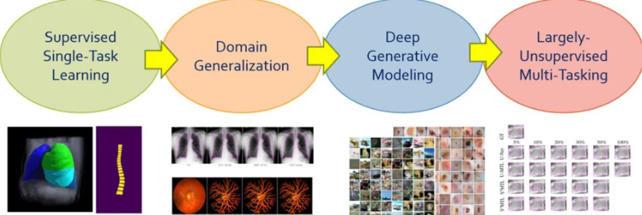
Figure 1.3: Spectrum of thesis contributions. Our contributions progress from supervised, single-task learning to sparingly-supervised multi-task learning.
1.4
Contributions
As illustrated in Figure 1.3, the contributions reported in this thesis range from
fully-supervised, single-task to sparingly-fully-supervised, multi-task deep learning, through domain generalization and deep generative modeling. In greater detail, the six contributions are as follows:
1. Volumetric medical image segmentation: Automatic, reliable lung lobe
seg-mentation is crucial to the diagnosis, assessment, and quantification of pulmonary diseases. Existing pulmonary lobe segmentation techniques are prohibitively slow, undesirably rely on prior (airway/vessel) segmentation, and/or require user in-teractions for optimal results. To address the need for accurate and robust lobe segmentation, we have pursued a fully automatic and reliable deep learning solution based on a Progressive Dense V-Network (PDV-Net). Our 3D PDV-Net model inputs an entire CT volume and generates accurate segmentation of the lung lobes in about 2 seconds in only a single forward pass of the network, eliminating the need for any user interaction or any prior segmentation of the lungs, vessels, or airways, which are common assumptions in the design of existing models. An extensive robustness analysis of our method demonstrates reliable lobe segmentation of both healthy and pathological lungs in CT images acquired by scanners from different vendors, across various CT scan protocols and acquisition parameters. This work is
published in (Imran et al.,2018, 2019a).
2. 2D medical image segmentation & disease quantification: Scoliosis is a
congenital disease in which the spine is deformed from its normal shape. Mea-surement of scoliosis requires labeling and identification of vertebrae in the spine. Spine radiographs are the most cost-effective and accessible modality for imaging the spine. Reliable and accurate vertebrae segmentation in spine radiographs is crucial in image-guided spinal assessment, disease diagnosis, and treatment planning. Conventional assessments rely on tedious and time-consuming manual measurement, which is subject to inter-observer variability. A fully automatic method that can accurately identify and segment the associated vertebrae is unavailable in the litera-ture. Leveraging a carefully-adjusted U-Net model with progressive side outputs, we propose an end-to-end segmentation model that provides a fully automatic and reliable segmentation of the vertebrae associated with scoliosis measurement. Our experimental results from a set of anterior-posterior spine X-Ray images indicate that our model, which achieves an average Dice score of 0.993, promises to be an effective tool in the identification and labeling of spinal vertebrae, eventually helping doctors in the reliable estimation of scoliosis. Moreover, estimation of Cobb angles from the segmented vertebrae further demonstrates the effectiveness of our model. This work is published in (Imran et al.,2019c, 2020a).
3. Deep generative modeling for simultaneous image generation and
classi-fication: From relatively small corpora of training data, deep generative models can
learn to generate realistic images approximating real-world distributions. In particu-lar, the proper training of Generative Adversarial Networks (GANs) and Variational AutoEncoders (VAEs) enables them to perform semi-supervised image classifica-tion. Combining the power of these two models, we introduce Multi-Adversarial Variational autoEncoder Networks (MAVENs), a novel deep generative modeling that incorporates an ensemble of discriminators in a VAE-GAN network in order to perform simultaneous adversarial learning and variational inference. We apply
MAVENs to the generation of synthetic images and propose a new distribution measure to quantify the quality of these images. Our experimental results with only 10% labeled training data from the computer vision and medical imaging domains demonstrate performance competitive to state-of-the-art semi-supervised models in simultaneous image generation and classification tasks. This work is published in (Imran and Terzopoulos, 2019a, 2021).
4. Generalized and improved medical image segmentation: The performance
of fully-supervised models for various image analysis tasks (e.g., anatomy or le-sion segmentation from medical images) is limited to the availability of massive amounts of labeled data. Given small sample sizes, such models are prohibitively data biased with large domain shift. To tackle this problem, we propose a novel end-to-end medical image segmentation model, namely Progressive Adversarial Semantic Segmentation (PASS), which can make improved segmentation prediction without requiring any domain-specific data during training time. Our extensive experimentation with 8 public diabetic retinopathy and chest X-ray image datasets, confirms the effectiveness of PASS for accurate vascular and pulmonary segmen-tation, both for in-domain and cross-domain evaluations. This work appears in (Imran and Terzopoulos, 2020).
5. Semi-supervised multi-task learning: We propose a novel multi-task learning
model for jointly learning a classifier and a segmentor, from chest X-ray images, through semi-supervised learning. In addition, we propose a new loss function that combines absolute KL divergence with Tversky loss (KLTV) to yield faster convergence and better segmentation performance. Based on our experimental results using a novel segmentation model, an Adversarial Pyramid Progressive Attention U-Net (APPAU-Net), we hypothesize that KLTV can be more effective in improving generalizability of multi-task learning models while being competitive in segmentation-only tasks. This work is published in (Imran and Terzopoulos,2019b).
6. Self-supervised, semi-supervised, multi-task learning: Leveraging adversar-ial training and self-supervision, we propose a novel general purpose semi-supervised, multiple-task model—namely, self-supervised, semi-supervised, multi-task learning (S4MTL)—for accomplishing two important tasks in medical imaging, segmentation
and diagnostic classification. Experimental results on chest and spine X-ray image datasets suggest that our S4MTL model significantly outperforms semi-supervised single task, semi/fully-supervised multi-task, and fully-supervised single-task models, even with a 50% reduction of class and segmentation labels. We hypothesize that our proposed model can be effective in tackling limited annotation problems for joint training, not only in medical imaging domains, but also for general-purpose vision tasks. This work is published in (Imran et al., 2020c).
1.5
Overview
The remainder of this dissertation is organized as follows:
Chapter 2 briefly reviews the developments in supervised learning, semi-supervised
learning, deep generative modeling, self-supervision, multitasking, and domain general-ization, especially applied to medical image segmentation, image synthesis, and image classification. We also review related work on applications such as pulmonary lobe seg-mentation from chest CT, measurement of scoliosis from spine radiographs, simultaneous image generation and classification, semi-supervised multitasking for combined image classification and segmentation, and improved segmentation with domain generalization without domain-specific data.
Chapter 3 develops the deep learning models and associated algorithms, ranging from fully-supervised, single-task learning to scarcely-supervised, multi-task learning, which were described in the previous section and Figure 1.3.
Chapter 4presents an extensive collection of experimental results with our proposed
algorithms and models. Appendix A describes all the datasets used, data insights, class distributions, and dataset partitionings for training, testing, and validation.
Chapter 5 concludes the dissertation with a summary of our work and promising
CHAPTER 2
Related Work
We will now review prior work relevant to the six contributions listed in the previous chapter. The material in this chapter is organized into two parts; first we review supervised learning approaches to medical image segmentation followed by approaches requiring only limited supervision.
2.1
Supervised Learning for Medical Image Segmentation
Image segmentation can classically be defined as the partitioning of an image into non-overlapping, coherent regions that are homogeneous based on some characteristic such as intensity or texture (Gonzalez et al., 2004). Image segmentation is usually considered the most important part of medical image analysis as it extracts regions of interest (ROI) and simplifies the representation by focusing attention to smaller regions crucial to disease diagnosis/prognosis. Segmentation simply assigns labels to a set of constituent regions, whereas semantic segmentation understands and recognizes image regions at the pixel level; i.e., semantic segmentation assigns class labels to each pixel in an image. In this section, we review related work on fully-supervised learning approaches semantic segmentation in general and prior deep learning methods for the segmentation of anatomical structures from 2D (e.g., X-rays) and 3D (e.g., CT scans) medical image data.
With the advent of deep convolutional neural networks (CNNs) in computer vision and medical image analysis, automatic feature learning algorithms via deep learning emerged for medical image segmentation. These methods perform segmentation via pixel-wise classification, overcoming the limitations of the conventional pixel or super-pixel based
methods requiring hand-crafted features (Mehra and Neeru,2016). CNNs employed in medical image segmentation can be categorized into two approaches: patch-wise and whole image-based processing. Ciresan et al.(2012) proposed a patch-wise sliding window-based convolutional network for the automatic segmentation of neuronal membranes in electron microscopy images. Kamnitsas et al. (2017) proposed a dual pathway 3D CNN architecture with a fully connected random field (CRF) for refining patch-based brain lesion segmentation from multi-channel MRI patient data. Long et al. (2014) proposed semantic segmentation using an end-to-end fully convolutional network (FCN) by transforming classification networks (Krizhevsky et al.,2012;Simonyan and Zisserman, 2014; Szegedy et al., 2015). This opened up the pixel-wise classification over the full images differing the earlier patch-wise, sliding window strategies. The fully-connected layers from the classification networks were replaced by convolution layers which allowed the model perform dense prediction (pixel-to-pixel) on arbitrary sized inputs and outputs. Moreover, coarse, high layer information were combined with fine, low layer information which resulted in predicting finer details.
Ronneberger et al. (2015a) proposed the U-Net architecture for biomedical image segmentation which won the ISBI 2015 cell tracking challenge. The architecture employs a contraction path for capturing context and a symmetric expansion path for the precise localization of object(s) of interest. At every layer of the expansion path, high resolution features from the contraction layer are combined in order to reconstruct it and achieve better segmentation prediction. Gu et al. (2019) proposed a context encoder network (CE-Net) that captures more high-level information while preserving spatial information, and applied the model to several 2D medical image segmentation applications (vessel detection, lung segmentation, etc.).
Extending the previous U-Net architecture, C¸ i¸cek et al. (2016) proposed the 3D U-Net for volumetric segmentation of Xenopus kidney. Replacing the 2D operations by their 3D counterparts, the 3D U-Net model was applied in semi-automated and automated setup for dense prediction in volumetric images. (Milletari et al., 2016) proposed a 3D CNN model namely V-Net for the segmentation of prostate volumes in MR images. To optimize
the training, a Dice-based objective function was proposed which deals with the imbalance between the number of foreground and background voxels. Each of the compression and decompression stages learns a residual function that ensures faster convergence.
By extracting intra-slice features with a 2D DenseU-Net and hierarchically aggre-gating volumetric contexts with a 3D DenseU-Net, Li et al. (2018) proposed a hybrid H-DenseUNet for liver and tumor segmentation from CT volumes.
Among different variants of the U-Nets and V-Net, attention U-Net (Oktay et al., 2018), nested U-Net (Zhou et al., 2019), hierarchical 3D U-Net (Roth et al., 2017) and 3D dense V-Net for abdominal segmentation(Gibson et al., 2018) are noteworthy.
2.1.1 3D Segmentation
Our work on 3D segmentation (Imran et al., 2018, 2019a), which is developed in Sec-tion 3.1.1, focuses on the segmentation of pulmonary lobes in 3D CT images of the
chest. We will next discuss the lung lobe segmentation problem and review the relevant literature.
Human lungs are divided into five lobes. The inner membrane of the lung (visceral pleura) folds towards the center of the lung and creates double layer fissures that define the five lobes. The lobar boundaries are made of two major (oblique) fissures and a minor (horizontal) fissure. As shown in Figure 2.1, the left lung has two lobes separated by a major fissure—the upper (superior) lobe and the lower (inferior) lobe. Along with upper and lower lobes, the right lung has a middle lobe; a minor fissure separates the upper lobe from the middle lobe and a major fissure separates the lower lobe from the middle lobe. Each of the five lobes is functionally independent, with its own bronchial and vascular systems.
Automatic segmentation of the lung lobes is important for both clinical and technical purposes. From the clinical perspective, automatic lung lobe segmentation can help radiologists review chest CT scans more efficiently. This is because radiologists often report their pulmonary findings by indicating the affected lung lobe, whose identification
Figure 2.1: An axial lung CT slice with visible fissures. In the left lung, the left upper lobe (LUL) and left lower lobe (LLL) are defined by a major fissure (indicated by red arrows). In the right lung, the right upper lobe (RUL), right middle lobe (RML), and right lower lobe (RLL) are defined by a major fissure (indicated by red arrows) and a minor fissure (indicated by yellow arrows).
requires them to navigate through the nearby slices and search for fissure lines, which are often visually indistinct. Automatic lung lobe segmentation can eliminate the need for such a tedious and time-consuming process. From the technical perspective, accurate lung lobe segmentation can assist several subsequent clinical tasks, including nodule malignancy prediction (cancers mostly occur in the left or right upper lobes), automatic lobe-aware report generation for each nodule (see Figure 2.2), and assessment and quantification of chronic obstructive pulmonary diseases (COPD) and interstitial lung diseases (ILD), by narrowing down the search space to the lung lobes most-likely to be affected.
However, identifying fissures poses a challenge for both human and machine perception. First, fissures are most often incomplete, not extending to the lobar boundaries. This is shown in Figure 2.2 where the horizontal fissure is incomplete, unlike the oblique fissures. Several studies in the literature have confirmed the incompleteness of fissures as a very common phenomenon. After reviewing 100 fixed and inflated lung specimens, Raasch et al.(1982) found incomplete right major fissures in 70% of the cases, left major in 46%
(a) (b)
(c) (d)
Figure 2.2: (a) A coronal slice where the major fissures are complete and visible, but the minor fissure (circled) is incomplete. (b) Nodule shown in the bounding box. (An example nodule report: 5mm nodule found in the left upper lobe). (c) Accessory fissure (arrows) in a left lung sagittal slice, which looks similar in shape to a minor fissure. (d) Azygos fissure (arrow) in an axial slice creates an extra lobe (azygos lobe) in the right
lung.
of the cases, and 94% across the minor fissures. Moreover, the studies of Gulsun et al. (2006) and Aziz et al. (2004) also showed more than 50% incompleteness in pulmonary fissures. Second, the visual characteristics of lobar boundaries change in the presence of pathologies. The changes could also be related to their thicknesses, locations, and shapes. Third, there also exist other fissures in the lungs that can be misinterpreted as the major and minor fissures that separate the lobes. Examples include accessory fissures (sagittal slice in Figure 2.2) and azygos fissures (axial slice in Figure 2.2).
automatic techniques. We categorize these approaches into two groups: reliant approaches, which rely on a prior segmentation or anatomical information, and non-reliant approaches, which do not rely on such prior segmentations.
2.1.1.1 Prior-Based Segmentation
Reliant approaches require as input a segmentation mask of lungs or lobes (different modalities), airways and vessels, or fissure initialization. A good example of the latter is the work by Doel et al. (2012), in which lobe segmentation is performed based on an initialization via fissure detection. In another example of fissure initialization,Iwano et al. (2013) proposed semi-automatic and automatic lobe segmentation methods based on region-growing. The semi-automatic approach requires major and minor fissure initialization, whereas for the automatic approach, recognition of lobar bronchi and localization of fissures are performed prior to the final lobar segmentation. On average, the semi-automatic approach takes approximately 80 seconds and the automatic approach takes approximately 44 seconds per case.
A number of works depend on prior segmentation of airways, vessels, or fissures. The work by Bragman et al. (2017) is a good representative, wherein the method relies on the prior segmentation of airways and vessels. Specifically, a population model of fissure priors was constructed and combined with patient-specific anatomical information for non-parametric surface fitting. Despite the promising results, the model lacks robustness and its reliance on prior knowledge limited the study. In recent work,Giuliani et al.(2018) proposed an approach to segment lobes from an approximate segmentation based on the airway tree. The final lobe segmentation was generated by combining the approximate seg-mentation with all the lung structures (airways, vessels, lungs, and fissures) segseg-mentation using a multilevel graph cut algorithm. This segmentation method is highly reliant on the quality of the prior airway and vessel segmentations, as well as anatomical knowledge. Lassen and van Rikxoort (2013) proposed a watershed-based lobe segmentation method by combining anatomical information from lungs, fissures, vessels, and bronchi. Despite
reporting improved segmentation in the presence of incomplete fissures, the failure of individual prior segmentations limited the performance of the overall segmentation. Based on this work, Lassen-Schmidt et al. (2017) proposed an interactive lobe segmentation method to interactively correct lobe segmentation error through user inputs. However, this improvement was obtained at the price of prolonged segmentation sessions. Lim et al. (2016) performed quantification of emphysema in 66 patients with moderate to severe emphysema who had undergone CT for lung volume reduction planning. They used lobar segmentation from four different prototypes for inter-software variability in lobe-wise emphysema quantifications. Although the lobe segmentation performance is not reported, it is dependent on prior airway and vessel segmentation.
Other works also rely on prior lung or lobe segmentation masks. For example, Bauer et al. (2018) segmented the lung lobes in the expiration phase based on a prior lobe segmentation mask obtained from a CT image acquired in the inspiration phase. An automated lung and lobe segmentation pipeline was proposed by Blaffert et al. (2010), in which a lung model mesh based on watershed segmentation is adapted to lobar segmentation. Final lobe regions are obtained by adjusting based on overlaid lungs in a post-processing step. However, the authors do not report a quantitative evaluation of lobar segmentation. The model takes 20 seconds to perform lobar segmentation in each CT scan.
2.1.1.2 Atlas-Based Segmentation
Another variation of reliant segmentation is registration using mutual information with a previously segmented atlas. The performance of final lobe segmentation is greatly dependent on the performance of the segmentation algorithm used in creating a reference atlas. Among atlas-based approaches for lobe segmentation, Ross et al. (2010) employed the thin-plate spline and a maximum a posteriori estimation method using a manually-defined atlas as a reference. Fissure points were selected based on the atlas and the final lobe segmentation was generated after a post-processing step. Although this method
does not rely on any prior airway and vessel segmentation, the execution time was long. Moreover, the creation of the atlas is very cumbersome and prone to poor results in pathological lung cases. By contrast, Pu et al. (2009) performed lobe segmentation by fitting an implicit function to fissures without reliance on prior airway or vessel segmentation. Although they achieved good accuracy for healthy lungs, the performance of their method degraded in the case of lungs with abnormal orientations. Unlike the other atlas-based segmentations, van Rikxoort et al. (2010) made use of multiple atlases for lobe segmentation. Their method showed promise albeit at the expense of slow execution.
2.1.1.3 Non-Reliant Segmentation
Recently, a few convolutional neural-network-based lobe segmentation techniques have been proposed (George et al., 2017; Ferreira et al., 2018; Wang et al., 2018). The segmentation method of George et al.(2017) employs a 2D fully convolutional network followed by a 3D random walker algorithm. This approach does not rely on a prior segmentation of airways or vessels nor on any pre-computed atlases; however, it cannot generate lobe segmentation in a single pass, nor in an end-to-end manner. Furthermore, the 3D random walker algorithm relies on a number of heuristics for the initialization of seeds and weights. Ferreira et al. (2018) proposed a lobe segmentation model based on a fully regularized V-Net model with deep supervision and carefully chosen regularization. Although the performance looks impressive, the model was trained with few examples, so it lacks generalizability and may not be effective for varying CT scan cases. A 3D Dense Net-based lobe segmentation method was proposed byWang et al. (2018). Although they reported good accuracy for pathological lungs, their lobe segmentation method relies on prior lung segmentation and assumes the presence of five lobes, which might not always be the case (e.g., (LOLA11, 2011)).
Our work (Imran et al., 2018, 2019a), developed in the next chapter, mitigates the aforementioned limitations—namely, reliance on prior masks, slow runtime, and lack of robustness—through an end-to-end learning network. Without relying on any prior
airway/vessel segmentation or anatomical knowledge or atlases, our method performs lobe segmentation in a single pass of the network. Owing to the full utilization of the 3D context in our model, the resulting lobe segmentation is smooth and nearly noise-free, which eliminates the need for any subsequent post-processing to fill holes or remove noisy patches from outside the lung area. Our method shows promise for the potential clinical use in quantification of pulmonary diseases and automatic generation of radiological reports.
2.1.2 2D Segmentation
In this section, we review the literature relevant to our work on the segmentation of vertebrae in 2D spinal X-ray images and the development of a segmentation-based pipeline for the measurement and analysis of scoliosis (Imran et al.,2019c,2020a), which is reported in Section 3.1.2.
Scoliosis is an abnormal condition defined by spinal curvature towards the left or right. Early detection is key and, when accurate, it can lead to better treatment planning (Weinstein et al., 2008). Radiography (X-Ray) is the preferred imaging technique for clinical analysis and measurement of scoliosis as it is highly available, inexpensive, and yields quick results. Conventional spine image analysis tasks involve tedious manual labor with hand-crafted feature extraction for the measurement of scoliosis. The Cobb angle, the standard metric of scoliosis, is estimated by calculating the angle between the two tangents of the upper and lower end plates of the upper and lower vertebrae. A person with a 10◦ or greater Cobb angle is usually considered for scoliosis diagnosis (Kim et al., 2010). Figure 2.3 illustrates the procedure for the calculation of the Cobb angle through the labeling of relevant vertebrae in an X-Ray image.
Conventionally, measurement and assessment, which requires the identification and labeling of specific vertebral structures, is manually performed by clinicians. However, the manual measurement of scoliosis faces several difficulties. First, large anatomical variation between patients and low tissue contrast in spinal X-Ray images make it challenging to
Apex
Cobb angle
T12
L1
L5
T1
C7
T11
L2
L3
L4
T10
T2
T9
T3
T4
T5
T6
T7
T8
Figure 2.3: Illustration of the Cobb angle calculation in an anterior-posterior spine X-ray, by selecting the most tilted upper vertebra above the apex and the most tilted lower vertebra below the apex. From the extended upper edge of the upper vertebra and lower edge of the lower vertebra, tangents are drawn and the intersection angle is calculated as the Cobb angle.
accurately and reliably assess the severity of scoliosis (Wu et al.,2017), and effects on the spine and body as a whole, as well as on individual vertebra, pose extra difficulty in the quantification of scoliosis (Kawchuk and McArthur,1997). Second, measurement error is prevalent in the routine clinical assessment of scoliosis due to instrumentation, vertebral rotation, and patient positioning (Kim et al., 2010), and 5◦–10◦ intra- or greater inter-observer variation has commonly been reported in measuring the Cobb angle (Beauchamp et al., 1993; Pruijs et al., 1994).
While several methods for vertebrae segmentation and scoliosis measurement are available, this approach is still under-explored in the literature. Existing vertebrae segmentation methods rely on manual interaction (Mateusiak and Mikolajczyk, 2019), hand-crafted feature engineering limited to customized parameters (Taghizadeh et al., 2019; Anitha and Prabhu, 2012), follow patch-based approaches that lose full spatial context (Qadri et al.,2019;Horng et al.,2019), are limited in scope and fail to consider all the required vertebrae at a time (Lessmann et al., 2019), etc. For Cobb angle estimation, a minimum bounding rectangle was used for the patch-wise segmented vertebrae (Horng et al., 2019), an approach that relies on pre-processing steps including spinal region isolation and vertebrae detection. Kusuma (2017) proposed a K-means and curve-fitting approach for Cobb angle measurement that requires a set of pre-processing steps (Kusuma, 2017). Other Cobb angle estimation methods have been proposed based on directly finding vertebrae corners as a form of regression task (Wu et al., 2018;Sun et al.,2017; Imran et al., 2019b; Wu et al.,2017). Although promising, these supervised methods are less viable for clinical applications because of low accuracy, due to the loss of fine details in the process, and the lack of explainability.
2.2
Limited Supervision
The scarcity of labeled or annotated medical image data and/or access to substantial quantities of unlabeled data motivates efforts to train deep learning models with limited supervision. We review the literature on limited supervision, including semi-supervised
learning facilitated by deep generative modeling, adversarial learning, self-supervision, multi-task learning, and domain generalization techniques, in the following sections.
2.2.1 Semi-Supervised Learning
Semi-supervised learning has recently been explored both in computer vision and medical imaging due to the availability of vast amounts of unlabeled data and computing power to process them. Semi-supervised learning is usually performed with a small portion of labeled and a larger portion of unlabeled data, assuming that both are from the same or similar distributions. In standard protocols, semi-supervised models are evaluated by retaining only a portion of the labels from a dataset while the remainder are treated as unlabeled data (Zhai et al., 2019). Depending on the approach to gaining information from large quantities of unlabeled data, semi-supervised learning can be performed in at least two different ways—self-supervised learning and adversarial training.
Self-supervised learning is similar to unsupervised learning in its goal of using a vast amount of unlabeled data to learn visual representation without any human annotation. Usually, self-supervised learning is performed by formulating a pretext or surrogate task only on the unsupervised data portion. Examples of pretext tasks could include image reconstruction, image colorization, predicting image rotations, etc. In self-supervision, the data itself lends to supervision; i.e., proxy labels created from the data on which training can provide useful visual features from unlabeled data. Tajbakhsh et al. (2019a) showed the effectiveness of training models from pre-trained surrogate tasks in different medical imaging applications, including diabetic retinopathy classification, nodule detection, and lung lobe segmentation with limited labeled data. Moreover, without training separately, both the pretext and downstream tasks can be combined in jointly learning useful visual features. Tran(2019) proposed a semi-supervised learning scheme based on self-supervised regularization, where the model is trained like full-supervision—a supervised branch for the labeled data and a self-supervised branch for the unlabeled data—to predict some geometric transformations.
Adversarial learning is closely related to the Generative Adversarial Networks (GANs) Goodfellow et al. (2014). In adversarial learning, class labels are augmented with an additional label to distinguish generated data from real data. A well balanced generator-discriminator helps towards learning useful visual features from the unlabeled data Donahue et al. (2016). Adversarial learning can effectively be adapted to semi-supervised learning for classification of both natural and medical images (Salehinejad et al., 2018; Imran and Terzopoulos,2019a). Adversarial learning has also been utilized in segmentation (semantic-aware generative adversarial nets (Chen et al., 2018), structure correcting adversarial nets (Dai et al.,2018), etc.) as well as in disease classification (semi-supervised domain adaptation (Madani et al., 2018), attention-guided CNN (Guan et al., 2018)).
2.2.2 Deep Generative Modeling
With the advent of deep generative models such as Variational AutoEncoders (VAEs) (Kingma and Welling, 2013) and Generative Adversarial Networks (GANs) (Goodfellow et al., 2014), the ability to learn underlying data distributions from training samples has become practical in common scenarios where there is an abundance of unlabeled data. With minimal annotation, efficient semi-supervised learning could be the preferred approach (Imran and Terzopoulos,2019b). More specifically, based on small quantities of annotation, realistic new training images may be generated by models that have learned real-world data distributions (Figure 2.4a). Both VAEs and GANs may be employed for
this purpose.
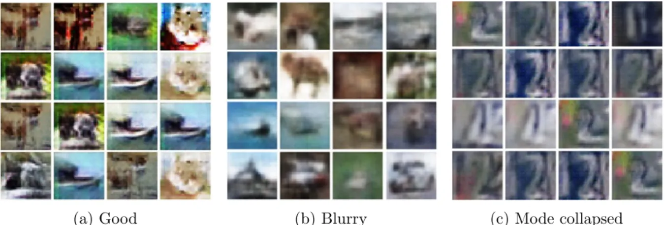
VAEs can learn dimensionality-reduced representations of training data and, with an explicit density estimation, can generate new samples. Although VAEs can perform fast variational inference, VAE-generated samples are usually blurry (Figure 2.4b). On the
other hand, despite their successes in generating images and semi-supervised classifications, GAN frameworks remain difficult to train and there are challenges in using GAN models, such as non-convergence due to unstable training, diminished gradient issues, overfitting, sensitivity to hyper-parameters, and mode collapsed image generation (Figure2.4c).
(a) Good (b) Blurry (c) Mode collapsed Figure 2.4: Image generation based on the CIFAR-10 dataset (Krizhevsky and Hinton, 2009): (a) Relatively good images generated by a GAN. (b) Blurry images generated by a VAE. Based on the SVHN dataset (Netzer et al., 2011): (c) Mode collapsed images generated by a GAN.
Several techniques have been proposed to stabilize GAN training and avoid mode collapse. Nguyen et al.(2017) proposed a model where a single generator is used alongside dual discriminators. Durugkar et al. (2016) proposed a model with a single generator and feedback aggregated over several discriminators, considering either the average loss over all discriminators or only the discriminator with the maximum loss in relation to the generator’s output. Neyshabur et al. (2017) proposed a framework in which a single generator simultaneously trains against an array of discriminators, each of which operates on a different low-dimensional projection of the data. Mordido et al.(2018), arguing that all the previous approaches restrict the discriminator’s architecture thereby compromising extensibility, proposed the Dropout-GAN, where a single generator is trained against a dynamically changing ensemble of discriminators. However, there is a risk of dropping out all the discriminators. Feature matching and minibatch discrimination techniques have been proposed (Salimans et al., 2016) for eliminating mode collapse and preventing overfitting in GAN training.
Realistic image generation helps address problems due to the scarcity of labeled data. Various architectures of GANs and their variants have been applied in ongoing efforts to improve the accuracy and effectiveness of image classification. The GAN framework has been utilized as a generic approach to generating realistic training images that synthetically
augment datasets in order to combat overfitting; e.g., for synthetic data augmentation in liver lesions (Frid-Adar et al., 2018), retinal fundi (Guibas et al., 2017), histopathology (Hou et al., 2017), and chest X-rays (Salehinejad et al., 2018; Imran and Terzopoulos, 2019b). Calimeri et al. (2017) employed a LAPGAN (Denton et al., 2015) and Han et al. (2018) used a WGAN (Arjovsky et al., 2017) to generate synthetic brain MR images. Bermudez et al. (2018) used a DCGAN (Radford et al., 2015) to generate 2D brain MR images followed by an autoencoder for image denoising. Chuquicusma et al. (2018) utilized a DCGAN to generate lung nodules and then conducted a Turing test to evaluate the quality of the generated samples. GAN frameworks have also been shown to improve the accuracy of image classification via the generation of new synthetic training images. Frid-Adar et al. (2018) used a DCGAN and an ACGAN (Odena et al., 2017) to generate images of three liver lesion classes to synthetically augment the limited dataset and improve the performance of a convolutional neural net (CNN) in liver lesion classification. Similarly, Salehinejad et al. (2018) employed a DCGAN to artificially simulate pathology across five classes of chest X-rays in order to augment the original imbalanced dataset and improve the performance of a CNN in chest pathology classification.
The GAN framework has also been utilized in semi-supervised learning architectures to leverage unlabeled data alongside limited labeled data. The following efforts demonstrate how incorporating unlabeled data in the GAN framework has led to significant improve-ments in the accuracy of image-level classification: Madani et al. (2018) used an order of magnitude less labeled data with a DCGAN in semi-supervised learning yet showed comparable performance to a traditional supervised CNN classifier and furthermore demonstrated reduced domain over-fitting by simply supplying unlabeled test domain images. Springenberg (2015) combined a WGAN and CatGAN (Wang and Zhang,2017) for unsupervised and semi-supervised learning of feature representation of dermoscopy images.
Despite the aforecited successes, GAN frameworks remain challenging to train, as we discussed above. Our MAVEN framework (Imran and Terzopoulos, 2019a, 2021), which we develop in Section3.2.1, mitigates the difficulties of training GANs by enabling training
on a limited quantity of labeled data, preventing overfitting to a specific data domain source, and preventing mode collapse, while supporting multiclass image classification.
2.2.3 Domain Generalization
The domain shift problem is usually mitigated using two approaches: unsupervised domain adaptation and domain generalization. Domain generalization involves acquiring knowledge from an arbitrary number of related domains and applying it to previously unseen domains. In unsupervised domain adaptation, a model is pre-trained on similar tasks in some other domain(s) with labeled data, and the pre-trained model is then fine-tuned with a limited set of labeled data in the target domain. Domain adaption can also be performed to learn a generic representation where the model is fully-supervised for source data and unsupervised for data from the target domain (Yang et al.,2019;Zhuang et al., 2019). These methods typically rely on the availability of unlabeled (Chen et al., 2019; Huo et al., 2018) or even labeled data (Zhang et al., 2018b;Dou et al., 2018) for the target domain. Therefore, with the unavailability of labeled/unlabeled data from the target domains or disparate data distributions, such models become less useful.
Also, approaches are described in the literature for learning generalized albeit error-prone initial segmentation across domains and applying different techniques to improve the final segmentation. For example, post-processing approaches inconsistently improve segmentation results but require extensive parameter tuning (Kamnitsas et al., 2017) and error propagation before the post-processing (Larrazabal et al., 2019). ErrorNet is another method proposed recently that can learn error correction in a systematic manner via learning a prior distribution of the segmentation masks (Tajbakhsh et al., 2019b). However, all of these methods are based on explicit error propagation whether it is handcrafted or model-derived. This adds vulnerability to the models for segmentation prediction and might increase shifts across different application tasks. Moreover, the over-reliance on the post-processing or secondary error correction steps diminishes the quality of visual representation learning.
Departing from all the previous methods, we proposed the PASS model (Imran and Terzopoulos, 2020), which is developed in Section 3.2.2. PASS is end-to-end and fully automatic, devoid of any pre- or post-processing and explicit error designs (hand-crafted/systematic), and, most importantly, better generalized for tackling domain shifts in segmentation tasks.
2.2.4 Multitask Learning
Multitask learning (MTL) can be accomplished in several ways, such as learning from auxiliary tasks to support the main task (Liebel and K¨orner, 2018), learning to learn multitask models (Zhang et al., 2018a), joint learning of multiple tasks (Liu et al., 2019; Imran and Terzopoulos,2019b), etc. By performing multiple tasks, the domain-specific information in the training signals of related tasks is actually improved (Caruana, 1993). MTL is particularly useful for implicit data augmentation through better representation, focusing attention on the most relevant features, learning one task through another, and regularizing among them (Ruder, 2017).
The literature includes several efforts on performing multiple tasks within the same model. Several prior efforts address multitask learning with CNNs and generative modeling. Rezaei et al. (2018) combined a set of auto-encoders with an LSTM unit and an FCN as discriminator for semantic segmentation and disease prediction. Girard et al. (2019) used a U-Net-like architecture coupled with graph propagation to jointly segment and classify retinal vessels. Mehta et al. (2018) proposed a Y-Net, with parallel discriminative and convolutional modularity, for the joint segmentation and classification of breast biopsy images. Another multitasking model was proposed by Yang et al. (2017) for skin lesion segmentation and melanoma-seborrheic keratosis classification, using GoogleNet extended to three branches for segmentation and two classification predictions. Khosravan and Bagci(2018) used a semi-supervised multitask model for the joint learning of false positive reduction and nodule segmentation from 3D computed tomography (CT) images.
adversarial learning framework. These include our APPAU-Net model (Imran and Terzopoulos, 2019c), which is developed in Section 3.2.3, and our S4MTL model (Imran et al.,2020b), which is developed in Section3.2.4 and further incorporates self-supervision
CHAPTER 3
Models and Associated Learning Algorithms
This chapter develops our novel models and associated learning algorithms, first of the fully-supervised type and then of the semi-supervised type.
3.1
Fully-Supervised Learning Models
We target our supervised learning models to the tasks of fully automated pulmonary lobe segmentation in 3D CT 3D images of the chest and vertebra segmentation in anterior-posterior spine X-Ray images for the measurement of scoliosis.
3.1.1 3D Pulmonary Segmentation in Chest CT Images
3.1.1.1 Progressive Dense V-Net
Combining ideas from dense V-Networks (Gibson et al.,2018) and progressive holistically-nested networks (Harrison et al.,2017), we propose a new architecture—the Progressive Dense V-Network (PDV-Net), an end-to-end solution for organ segmentation in 3D volumetric data.
As shown in Figure3.1, the input to the network is first down-sampled and concatenated with a strided 5×5×5 convolution of the input with 24 kernels. The concatenation result is then passed to 3 dense feature blocks, each consisting of 5, 10, and 10 densely-wired convolution layers respectively. The growth rates of the dense blocks are set to 4, 8, and 16 respectively. All the convolutional layers in a dense block have a kernel size of 3×3×3 and are followed by batch normalization and parametric rectified linear units
Figure 3.1: PDV-Net model for the segmentation of lung lobes. Segmentation outputs in different pathways are progressively improved to yield the final result.
(PReLU). The outputs of the dense feature blocks are consecutively utilized in low and high resolution passes via convolutional down-sampling and skip connections. This enables the generation of feature maps at three different resolutions. The outputs of the skip connections of the second and third dense feature blocks are further up-sampled in order to be consistent with the size of the output in the first skip connection. The feature maps from skip1 are passed to a convolutional layer followed by a softmax, which outputs the probability maps. In the second pathway, the feature maps from skip1 and skip2 are merged and the output probability maps are produced by a convolutional layer followed by softmax. Similarly, we obtain the final segmentation from the merged feature maps resulting from the skip2 and skip3 connections. Unlike the dense V-Net, the PDV-Net generates the final output by progressively improving the outputs at previous pathways.
The PDV-Net is trained using a subsetSof a volumetric medical image datasetD. The training setScontains 3D CT scan images and their corresponding ground truth labels. So,
S = (Xn,Yn), forn = 1, . . . , N, where the input CT volumes X
(m)
n =x(in);i= 1, . . .|X |n,
and the corresponding ground truth labeled volumes Yn(m) = yi(n);i= 1, . . .|Y|n, y
(n)
Side outputs
Input X-Ray Vertebrae mask
Figure 3.2: Architecture of our segmentation network (Progressive U-Net): Side outputs at three different stages of the decoder are generated and progressively added to the next stage side-output. The output from the third side-output is added to the last stage before the final convolution to generate the final segmentation output.
{0. . . L}. Here, |S|is the total number of training examples passed to the network and
L is the number of labels provided in the ground truth data through per-voxel labeling (l). To train the PDV-Net, we use a Dice loss function (Milletari et al., 2016) at each level of the progressive network, which directly maximizes the similarity between the predicted values and the ground truth over all voxels. This loss properly handles the class imbalance problem prevalent in lung lobe segmentation: lung lobes have different sizes and background regions can be large. We employ a multi-class Dice for the segmentation task: d= L X l=1 PZ j=1p l jglj PZ j=1(p l j)2+ PZ j=1(g l j)2 , (3.1)
where Z is the total number of voxels,Lis the number of classes, plj denotes the predicted probabilities for each class, and gl
j denotes the corresponding ground truth for each class.
3.1.2 Segmentation and Scoliosis Quantification in Spine Radiographs
3.1.2.1 Vertebrae Segmentation and Labeling
We perform binary segmentation of the spine with a well-distinguishable number n of vertebrae relevant to scoliosis analysis. To formulate the problem, we assume an unknown data distributionp(X, Y) over imagesX and vertebrae segmentation labelsY. The model
Algorithm 1: Training for vertebrae segmentation in spine X-Ray images
Require:
Training data x, y ∈ D including spine X-Ray images x and reference vertebra segmentation masks y
Model architecture Fφ with learnable parameters φ
Ensure:
for each step over D do
Sample minibatch M: x(i) ∼pD(x)
Compute model outputs for the minibatch: ˆ
y(i) ← F(φ)(x)
Calculate loss L(y,yˆ) for the model predictions
Update the model F along its gradient
∇ψF 1 |M| X i∈M LF (y(i),yˆ(i)) end for
has access to the labeled training set D(x,y) sampled i.i.d. from p(X, Y). As shown in
Algorithm 1, the segmentation prediction networkFφ is trained with a set of learnable
parameters φ. We specify the objective as minφF L(y,yˆ), where yis the reference vertebrae mask and ˆy is the model prediction in each of the training iterations.
Following the progressive dense V-Net model (Imran et al., 2018, 2019a), we propose a progressive U-Net with some careful adjustments in the U-Net (Ronneberger et al., 2015b). As shown in Figure 3.2, our model has an encoder and a decoder with skip connections. In each encoder layer, two 3×3 convolutions are followed by instance normalization, ReLU activation, and a 2×2 max-pooling. A dropout is applied in every encoder and decoder stage of the network. We generate side-outputs in every stage of the decoder. Progressively adding one side-output to the next, the segmentation performance is improved compared to collecting the final output from the final decoder stage in a U-Net. However, one key difference with (Imran et al.,2018) is that our model is trained without side-supervision. Only the side-outputs are generated and added progressively, yielding an improved segmentation at the final output. A convolution operation is performed to generate the side-output from each decoder stage. The progressive side-outputs also ensure
Algorithm 2: Cobb angle calculation.
Input: Vertebra mask ˆy
Output: Cobb angleθ
From the predicted mask ˆy, get all the contours
for each contour in contours do if Number of pixels < a then
//to remove any noisy patches if there are any Remove contour
end if end for
//This will give n contours of well-separated vertebrae Extract four corner points from the vertebra contours Order the extracted 4n corners from bottom to top
for up = 1 to n−2do for low = up + 2 to n do
//with vertebra gap of 2
Determine slope of the upper edge of the upper vertebra (mup)
Determine slope of the lower edge of the lower vertebra (mlow).
Calculate Cobb angle, τ(up, low) = tan −1mup−mlow 1+mupmlow end for end for
Final Cobb angle, θ = max(τ)
that micro-structure is not lost from any level of the decoder through the convolutional operations. We generate side outputs at x/8, x/4, and x/2 resolutions before the final output atx resolution. Therefore, the side output at resolution x/8 is added to the next decoder stage, and so on.
3.1.2.2 Measurement of Scoliosis
Our pipeline makes use of the vertebrae segmentation in estimating Cobb angles. Al-gorithm2 automatically calculates the Cobb angle by analyzing the contours from the segmented mask. When well-separated from others, each of the contours represents a vertebra relevant to the measurement of scoliosis. To verify if a contour is actually associated to a relevant vertebra, we impose a minimum size on the number of contour pixels (a). After the extraction and ordering of the 4n corners, the most tilted upper