Department of Information Systems &
Computer Science Faculty Publications Department of Information Systems & Computer Science 2016
Improving the vector auto regression technique for time-series
Improving the vector auto regression technique for time-series
link prediction by using support vector machine
link prediction by using support vector machine
Proceso L. Fernandez JrJan Miles Co
Follow this and additional works at: https://archium.ateneo.edu/discs-faculty-pubs
Improving the vector auto regression technique for time-series link
prediction by using support vector machine
Jan Miles Co and Proceso Fernandez
Ateneo de Manila University, Department of Information Systems and Computer Science, Quezon City, Philippines
Abstract. Predicting links between the nodes of a graph has become an important Data Mining task because of its direct applications to biology, social networking, communication surveillance, and other domains. Recent literature in time-series link prediction has shown that the Vector Auto Regression (VAR) technique is one of the most accurate for this problem. In this study, we apply Support Vector Machine (SVM) to improve the VAR technique that uses an unweighted adjacency matrix along with 5 matrices: Common Neighbor (CN), Adamic-Adar (AA), Jaccard’s Coefficient (JC), Preferential Attachment (PA), and Research Allocation Index (RA). A DBLP dataset covering the years from 2003 until 2013 was collected and transformed into time-sliced graph representations. The appropriate matrices were computed from these graphs, mapped to the feature space, and then used to build baseline VAR models with lag of 2 and some corresponding SVM classifiers. Using the Area Under the Receiver Operating Characteristic Curve (AUC-ROC) as the main fitness metric, the average result of 82.04% for the VAR was improved to 84.78% with SVM. Additional experiments to handle the highly imbalanced dataset by oversampling with SMOTE and undersampling with K-means clusters, however, did not improve the average AUC-ROC of the baseline SVM.
1 Introduction
One of the major problems in network analysis involves predicting the existence or emergence of links given a network. The link prediction task has many practical applications in various domains. In biology, link prediction has been used for identifying protein-protein interaction [1] and for investigating brain network connections [2]. In social media, link prediction has been used for identifying both future friends and possible enemies by analyzing positive and negative links [3]. Efforts have also been made to apply link prediction techniques in communication surveillance to identify terrorist networks by monitoring emails [4].
Most of the previous works on link prediction use a static network to predict hidden or future links. In the detection of hidden links, the network is based on a known partial snapshot, and the objective is to predict currently existing links [4]. In the prediction of future links, the network is based on a snapshot at time t, and the objective is to predict links at time t’ (t’ > t) [5]. In this framework, insight regarding the dynamics of the network is disregarded, and information on the occurrence and frequency of links across time is lost. Hence, recent works on link prediction use a dynamic network where the network is characterized by a series of snapshots that represent the network across time [4, 5].
Some of the recent works on link prediction have also explored different ways to semantically enrich the network representation. A study was done by [6] that uses a heterogeneous network where nodes represent more than one type of entity. In the prediction of co-authorship networks, a node may represent an author, a topic, a venue or a paper. In another study done by [7], the network was formed by combining multiple layers of network formed by different types of nodes. In this case, the network model is composed of the following layers: the first layer is a co-authorship network; the second layer is a venue network, while the third layer is a co-citing network. The final homogeneous network is an aggregation of the three networks where nodes represent authors.
In this study, we focus on link prediction for a dynamic and homogeneous network. Since Vector Auto Regression (VAR) has been shown to be one of the best techniques for time-series link prediction [8], we incorporate some ideas from this technique and explore ways of improving the prediction. In particular, because the VAR model assumes a linear dependence of the temporal links on multiple time-series, we propose the use of Support Vector Machine (SVM) in order to more robustly handle a non-linear type of dependency even while retaining the assumption that the dependency is on multiple time-series. This paper describes our experimentation on this proposed idea.
2 Related Literature
In this section, we briefly review the literature on VAR model and its application in link prediction, the SVM model and its problems on imbalanced datasets, and some of the techniques applied for handling such imbalanced datasets.
2.1 Vector Auto Regression for Link Prediction
The VAR econometric model is an extension of the univariate autoregressive model that is applied to multivariate data. It provides better forecast than univariate time-series models and is one of the most successful models for analyzing multivariate time-series [9]. In a recent work on dynamic link prediction, the VAR technique was applied in homogeneous networks represented by both unweighted and weighted adjacency matrices. For each of the unweighted and weighted adjacency matrices, five additional matrices were created according to different similarity metrics. These metrics are the Number of Common Neighbor (CN), Adamic-Adar Coefficient (AA), Jaccard’s Coefficient (JC), Preferential Attachment (PA), and Resource Allocation Index (RA). Using a dataset created from DBLP, the performance of VAR was compared to static link prediction and to several dynamic link prediction techniques, which are Moving Average (MA), Random Walk (RW), and Autoregressive Integrated Moving Average (ARIMA). The VAR technique showed the best performance among the many link prediction techniques. For a more detailed discussion, refer to [8].
2.2 SVM and Imbalanced Datasets
Support Vector Machine (SVM) is a well-known learning model that is used mainly for classification and regression analysis. It computes for a maximum-margin hyperplane that separates the two classes of instances from a given dataset. The SVM does not necessarily assume that the dataset is linearly separable in the original feature space, and thus often uses the technique of projecting, via kernel trick, to higher-dimensional space where the instances are presumed to be more easily separable.
The SVM has been shown to be very successful in many applications including image retrieval, handwriting recognition, and text classification. However, the performance of SVM drops significantly when faced with a highly imbalanced dataset. A highly imbalanced dataset is characterized by instances from one class far outnumbering the instances from another class. This makes it difficult to classify instances correctly due to a small number of the sample size for one class [10]. This type of dataset is observed in our co-authorship network since there are significantly many potential co-authorship links and only few of these are realized.
2.3 SMOTE and SVM with Different Error Costs
In a work done by [10], three techniques were used to address the problem of highly skewed datasets. The first technique is to not undersample the majority instances, since doing otherwise leads to information loss. In the case of imbalanced datasets, the learned boundary of SVM tends to be too close to the positive instances. Hence, the second technique is to apply Different Error Costs (DEC) to different classes to force SVM to push the boundary away from the positive instances. The third technique is to apply Synthetic Minority Over-Sampling Technique (SMOTE) to make positive instances more densely distributed. Hence, making the boundary better defined. Ten (10) datasets where used to test the techniques. The performance of SVM with the original dataset was compared to the performance of the following techniques: SVM with undersampling, SVM with SMOTE, SVM with DEC, and SVM with a combination of SMOTE and DEC. In 7 out of 10 datasets, the best performance was achieved with a combination of SMOTE and DEC [10].
2.4 K-Means Clustering for Under-Sampling
K-means clustering is one of the simplest unsupervised learning algorithms and has been used by researchers to solve well-known clustering problems. In a work done by [11], K-means clustering was used as an undersampling technique for a highly imbalanced dataset. The training set was divided into two: the 1stset contains the minority instances, while the 2ndset contains the majority instances. The majority instances were partitioned into K clusters, for someK> 1. Each majority cluster was combined with the minority set to form a candidate training set, and the quality of the candidate training set was evaluated by using the Fuzzy Unordered Rule Induction Algorithm (FURIA). The best candidate training set was used for classification with C4.5 decision tree. This undersampling technique was applied to cardiovascular datasets from Hull and Dundee clinical sites. The proposed K-means undersampling method outperformed the use of the original dataset and the use of another K-means undersampling technique that was proposed by [12].
3 Methodology
3.1. Dataset
DBLP computer science bibliography contains bibliographic information on major computer science journals and proceedings. The co-authorship network in DBLP was used for the link prediction task. Following the dataset preparation in [8], we selected only the articles from 2003 to 2013, removing all items labelled as inproceedings, proceedings, book, incollection, phdthesis, masterthesis, and www. The reduced set was further trimmed by removing all authors who have 50 articles or less. The final dataset has 1,743 authors and 21,920 articles. The number of co-authorship links in this dataset is less than 1% of the total number of possible links.
p r u o i w 1 a e m c c • • • • • w 3 W b a u w v m m th s a f To bu partitioned resulting 1 up to 2013 of the dyn s represen wheren= 1 if the co article pub element is matrix for correspond commonly Number o Adamic-A Jaccard’s Preferent Resource whereΓ(x) 3.2 Basel We used t by [8], to adjacency using the f ˆ Yt A + + where each values for matrixCja model par he lm() fu set for each The VA authorship factors: th uild the ti d based on 11 subsets 3 (t=10), w amic co-a nted by an 1,743 (th orrespondi blished on s 0. Base each sna ding to y used for l of Commo CN x
(
,y Adar Coef AA x(
,y s Coefficie JC x(
, tial Attach PA x( )
,y e Allocatio RA x(
,y ) is the set line VAR the VAR t o form t matrix at formula: =Ct−1+αtA− +αt−1 PAYPA t−1 t−1+ +αt−2 AAYAA t−2 t−1+ hY j iis an the simila and scalar rameters. unction in h snapshot AR model link at e 6 metric ime-series n the year s, correspo was proce authorship nn×nunw e number ing two au the given ed from apshot, fiv the sim link predic on Neighb y)
= Γ( )
x fficient (A y)
= z∈Γ( )∑
x∩ ent (JC) ,y)
=Γ( )
x Γ( )
x hment (PA)
= Γ( )
x * on Index (R y)
= z∈Γ( )∑
x∩ t of nodes R and SVM technique the baseli timet, d −1Y A t−1+αt−1 CNY αt−1 RAYRA t−1 t−1+α αt−2 JCYJC t−2 t−1+α n n×nma arity metr r coefficien We appli R, to fin t. l describe time t is cs (includ s models, of public onding to ssed to ge network g weighted of author uthors hav n year, oth the unwe ve matrice milarity m ction: bor (CN) ∩Γ( )
y AA) 1 log(
Γ ∩Γ( )y∑
∩Γ( )
y ∪Γ( )
y A) Γ( )
y RA) 1 Γ( )
z ∩Γ( )y adjacent t M Models with lag ine mode denoted by YCN t−1 t−1+αt−1 AAY αt−2 AYA t−2 t−1+αtC− αt−2 PAYPA t−2 t−1+αtR− atrix repre ric iat tim ntsα j i are ed linear d the best d here ass linearly ding the ad the data ation. Eac years 20 enerate a s graph. A s adjacency rs), and an ve co-auth herwise th eighted ad es were co metrics th Γ( )
z)
o node (au s of 2, as p el. The p yYˆ t A, is co AA t−1 t−1+αt−1 JCYJC t− t− −2 CNYCN t−2 t−1 −2 RAYRA t−2 t−1 esenting th mej, and t e time-bas regressio t fitting pa sumes that dependen djacency aset was ch of the 03 (t=0) snapshot snapshot y matrix, n entry is hored an he matrix djacency omputed hat are (1) (2) (3) (4) (5) uthor)x. proposed predicted omputed C 1 1 (6) he actual the n×n sed VAR n, using arameter t the co-nt on 12 relation) from visua in Fig case. the d princi varian can im Figur VAR used t space instan Fo prese the 1 depen study dimen classi instan the p timet 3.3 B To co mode VAR for ti value finall at tim the V T Chara the pe Opera corre axis c are re 2 previou alization of gure 1, ind In this fig data. How ipal comp nce in the mprove th re 1.Data v and SVM m to project th by using th nces. or the SV nce or abs 12-dimensi ndency as y. These in nsion usin ifier is th nce, and th predicted a t. Benchma ompare the els, we app R (or SVM me t-1 an es at time y compare met+1. We VAR techn he Area acteristic erformanc ating Ch sponds to correspond espectively FPR us time p f the datas dicates tha gure, there wever, it ponents ac e dataset. e time-ser visualization models. Pri he 13-dimen he first two VM model sence of a ional feat ssumed in nstances w ng an SVM hen used hese predi adjacency arking e predictiv plied back M) model f ndt-2, the t+1 using ed the pre e were abl ique in 8 y a Unde Curve (A ce of the p haracteristi the False ds to the T y compute R= F FalsePo periods, t -set for the at this may e is no clea should b ccounted We explo ries predic n of the inst incipal Com nsional poi principal c l, each ins a co-autho ture space n the lag were furth M linear ke to predi ictions are matrix, ve powers ktesting. T for timetu en used th g values fr ediction ag le to meas years, from er the UC-ROC) redictive m ic (ROC e Positive True Posit ed as follow FalsePositi ositive+Tru Y 1 and t-2 snapshot y not nece an linear m be noted for just 5 ore SVM tion. tances from mponent An ints to the 2 components stance rep rship link e, followin 2 VAR m her projec ernel funct ct the cl e collected , of th s of the VA That is, w using the is model rom timet gainst the k sure the pe m Year 3 t Receiver ) was use models. In ) Curve, Rate (FPR tive Rate ws: ive ueNegative ˆ Yt A . Howeve t=2, as sho essarily be model that that the 58.3% of to verify mt=2, for th nalysis was 2-coordinate s of the presenting is mappe ng the lin model of cted to hig tion. An S lass for e d to const he network AR and S we first bu metric va to predict t andt-1, known va erformanc to Year 10 r Opera ed to mea n the Rece , the x -R) and th (TPR), wh ( er, a own e the t fits two the if it he e the ed to near this gher VM each truct k at VM ilt a alues t the and alues ce of 0. ating sure eiver axis hey -hich (7)TPR= TruePositive TruePositive+TrueNegative
(8)
The AUC of a perfect model is 1, while a random model will have an expected AUC of 0.5. In our context, positives correspond to links while negatives correspond to no links.
3.4 Further Experimentation on SVM
3.4.1 SMOTE and Different Error Cost
We were unable to apply the first approach proposed by [10] of not undersampling, due to the large sample size of our negative instances. For our first attempt to improve our baseline SVM, we applied the Different Error Costs (DEC) technique that was suggested by [10], which is setting the cost ratio to the inverse of the imbalance ratio. For our training set, we created an imbalanced ratio of 1:2 and set the error cost to 1 for positive links and 2 for negative links.
For our second attempt to improve our baseline SVM, we applied SMOTE, which was also suggested by [10]. To create the training sets, we oversampled the positive instances by 100% and undersampled our negative instances by selecting negative instances until we have equal number of positive and negative instances. Hence, we doubled the number of both positive and negative instances from our baseline SVM experiment.
For our third attempt to improve our baseline experiment, we combined the use of DEC and SMOTE. We used SMOTE to create an imbalance ratio of 1:2 and set the appropriate error costs. We performed the three experiments, then computed the AUC-ROC and compared this to our baseline SVM result.
3.4.2 K-Means Clustering
For our last attempt to improve our baseline SVM, we used K-means clustering, as proposed by [11], to under-sample the majority instances. First, we separated the positive instances from the negative instances. Then we clustered the negative instances into K = 2 clusters and selected the largest cluster. To form the training set, we performed random sampling in the larger cluster until we have an equal number of positive and negative instances. We combined the sampled majority instances to the
positive instances and used this dataset to train an SVM classifier. We evaluated the AUC-ROC and compared this to our baseline SVM result.
4 Results and Discussion
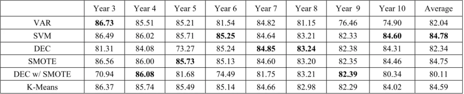
In this section, we present the result of our experiments in two parts: the result of comparing the performance of VAR technique and SVM classification algorithm and the result of our attempts to further improve our baseline SVM. The complete AUC-ROC results for all the experiments are shown in Table 1.
4.1. Baseline VAR and SVM models
SVM was able to outperform VAR with average AUC-ROC values of 84.78% and 82.04% respectively. A two-tailed pairedt-test was conducted in order to determine if there is significant difference in the means, with at least 90% confidence level. The resulting p-value of 0.064 suggests that there is a statistically significant difference.
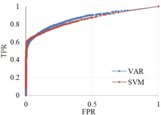
In 6 out of 8 years, SVM was able to achieve a better performance than VAR. Figure 2 shows a plot of the ROC of VAR and SVM for Year 10, the snapshot where the SVM was able to outperform VAR by the largest margin.
There were two snapshots where VAR was able to outperform SVM but these were only by small margins of 0.24 (in Year 3) and 0.18 (in Year 7). Figure 3 shows the ROC for Year 3.
The results suggest that the VAR model can be significantly improved by SVM classification algorithm when the VAR model multivariate time-series input data is used as the training set for linear SVM in the domain of time-series link prediction.
Figure 2. ROC of VAR and SVM in Year 10.
Table 1. AUC-ROC of Link Prediction Experiments.
Year 3 Year 4 Year 5 Year 6 Year 7 Year 8 Year 9 Year 10 Average
VAR 86.73 85.51 85.21 81.54 84.82 81.15 76.46 74.90 82.04 SVM 86.49 86.02 85.71 85.25 84.64 83.21 82.33 84.60 84.78 DEC 81.31 84.08 73.27 85.24 84.85 83.24 82.38 84.31 82.34 SMOTE 86.56 86.00 85.73 85.13 84.60 83.20 82.35 84.46 84.75 DEC w/ SMOTE 70.94 86.08 81.68 74.49 81.75 83.21 82.39 80.34 80.11 K-Means 86.37 85.74 85.49 85.14 84.66 82.98 82.29 84.02 84.59 4
Figure 3. ROC of VAR and SVM in Year 3.
4.2. Experiments to Improve Baseline SVM
In our subsequent experiments, we were unable to improve the average AUC-ROC of our baseline SVM despite implementing multiple techniques for handling the highly imbalanced dataset. In Table 1, we highlight the ROC for each year where the highest AUC-ROC was achieved. However, we were able to improve the performance of our baseline SVM in 6 out of 8 years. Each of the three techniques, SVM with DEC, SMOTE, and DEC with SMOTE, were able to improve the results in two years each. DEC was able to improve SVM by 0.21% and 0.03% in Years 7 and 8, while SMOTE was able to improve SVM by 0.07% and 0.02% in Years 3 and 5. Finally, DEC with SMOTE was able to improve SVM by 0.06% both in Years 4 and 9.
From our results, we hypothesize that the reason DEC, SMOTE, and DEC with SMOTE failed to improve the average performance of our baseline SVM is that the techniques were designed to perform well on not undersampled data as proposed by [10]. Although the techniques were able to improve our baseline SVM in a few individual years, the improvements were not consistent enough to beat the average performance of the baseline SVM.
SVM with undersampling by K-means clustering also failed to improve our baseline SVM. We infer that there is inherent information loss in random sampling from the larger majority instances cluster that leads to the poor performance of SVM with undersampling by K-means. However, in the case of datasets with noisy majority instances, undersampling by K-means clustering might improve classification as shown by [11].
5 Conclusion and Further Studies
In this study, we performed dynamic link prediction using various algorithms. Primarily, we were able to improve the performance of the VAR model by transforming its input multivariate time-series data as a feature set vector that was used as a training set to linear SVM. The VAR model was able to achieve an average AUC-ROC of 82.04% while SVM was able to achieve an AUC-ROC of 84.78%. This implies that the performance
of the VAR model can be improved by using SVM classification algorithm for dynamic link prediction.
In our attempt to further improve the performance of the baseline SVM, we experimented on several techniques such as SVM with different error costs (DEC), SMOTE, and undersampling by K-means clustering. In the case of un-noisy, large, and highly imbalanced datasets, we were forced to under-sample the majority instances, which might explain the poor performance of SVM with DEC, SMOTE, the combination of both techniques, and K-means clustering.
Based on these findings, we aim to improve other existing link prediction techniques by using other classification algorithms. We also intend to enrich our network model by using a weighted network and by using sematic information, which might result to better link prediction as shown in some previous works. Finally, we recommend further studies to improve oversampling and under-sampling techniques for binary classification specifically for link prediction, where dataset is often un-noisy, large, and highly imbalanced.
References
1. M. Kurakar, S. Izudheen. IJCTT 9,Link Prediction in Protein-Protein Networks: Survey, 164-168 (2014) 2. Y. Yang, H. Guo, T. Tian, H. Li. TST 20, Link
Prediction in Brain Network Based on Hierarchical Random Graph Model, 306-315 (2015)
3. J. Tang, S. Chang, C. Aggarwal, H. Liu. WSDM, Negative Link Prediction in Social Media(2015) 4. Z. Huang, D.K.J. Lin, INFORMS JOC21,The
Time-Series Link Prediction Problem with Application in Communication Surveillance, 286-303 (2009) 5. P.R. Soares, R.B. Prudencio, IJCNN, Time Series
Based Link Prediction(2012)
6. J.B. Lee, H. Adorna, ASONAM,Link Prediction in a Modified Heterogeneous Bibliographic Network (2015)
7. M. Pujari, R. Kanawati. NHM10,Link Prediction in Multiplex Networks (2015)
8. A. Ozacan, S.G. Oguducu. ICIS, Multivariate Temporal Link Prediction in Evolving Social Networks(2015)
9. P.D. Gilbert, IJF14,Combining VAR Estimation and State Space Mode Reduction for Simple Good Predictions. 229-250 (1995)
10. R. Akbani, S. Kwek, N. Japkowicz. ECML 3201, Applying Support Vector Machine to Imbalanced Datasets, 39-50 (2004)
11. M.M. Rahman, D.N. Davis. WCR 3, Cluster Based Under-Sampling for Imbalanced Cardiovascular Data(2013)
12. S.J. Yen, Y.S. Lee. ESWA 36, Cluster-Based Undersampling approaches for imbalanced data distributions, 5718-5727 (2009)