Device characterization

chapter five

Device characterization

Raja Balasubramanian

Xerox Solutions & Services Technology Center

Contents

5.2 Basic concepts

5.2.1 Device calibration 5.2.2 Device characterization

5.2.3 Input device calibration and characterization 5.2.4 Output device calibration and characterization 5.3 Characterization targets and measurement techniques

5.3.1 Color target design

5.3.2 Color measurement techniques 5.3.2.1 Visual approaches

5.3.2.2 Instrument-based approaches 5.3.3 Absolute and relative colorimetry 5.4 Multidimensional data fitting and interpolation

5.4.1 Linear least-squares regression 5.4.2 Weighted least-squares regression 5.4.3 Polynomial regression

5.4.4 Distance-weighted techniques 5.4.4.1 Shepard’s interpolation 5.4.4.2 Local linear regression 5.4.5 Lattice-based interpolation 5.4.6 Sequential interpolation 5.4.7 Neural networks 5.4.8 Spline fitting

270 Digital Color Imaging Handbook

5.6 Scanners

5.6.1 Calibration

5.6.2 Model-based characterization 5.6.3 Empirical characterization 5.7 Digital still cameras

5.7.1 Calibration

5.7.2 Model-based characterization 5.7.3 Empirical characterization

5.7.4 White-point estimation and chromatic adaptation transform

5.8 CRT displays 5.8.1 Calibration 5.8.2 Characterization 5.8.3 Visual techniques 5.9 Liquid crystal displays

5.9.1 Calibration 5.9.2 Characterization 5.10 Printers 5.10.1 Calibration 5.10.1.1 Channel-independent calibration 5.10.1.2 Gray-balanced calibration

5.10.2 Model-based printer characterization 5.10.2.1 Beer–Bouguer model

5.10.2.2 Kubelka–Munk model 5.10.2.3 Neugebauer model

5.10.3 Empirical techniques for forward characterization 5.10.3.1 Lattice-based techniques

5.10.3.2 Sequential interpolation 5.10.3.3 Other empirical approaches 5.10.4 Hybrid approaches

5.10.5 Deriving the inverse characterization function 5.10.5.1 CMY printers

5.10.5.2 CMYK printers

5.10.6 Scanner-based printer characterization 5.10.7 Hi-fidelity color printing

5.10.7.1 Forward characterization 5.10.7.2 Inverse characterization 5.10.8 Projection transparency printing 5.11 Characterization for multispectral imaging 5.12 Device emulation and proofing

5.13 Commercial packages 5.14 Conclusions Acknowledgment References Appendix 5.A Appendix 5.B

Chapter five: Device characterization 271

5.1 Introduction

Achieving consistent and high-quality color reproduction in a color imaging system necessitates a comprehensive understanding of the color character-istics of the various devices in the system. This understanding is achieved through a process of device characterization. One approach for doing this is known as closed-loop characterization, where a specific input device is opti-mized for rendering images to a specific output device. A common example of closed-loop systems is found in offset press printing, where a drum scan-ner is often tuned to output CMYK signals for optimum reproduction on a particular offset press. The tuning is often carried out manually by skilled press operators. Another example of a closed-loop system is traditional photography, where the characteristics of the photographic dyes, film, devel-opment, and printing processes are co-optimized (again, often manually) for proper reproduction. While the closed-loop paradigm works well in the aforementioned examples, it is not an efficient means of managing color in open digital color imaging systems where color can be exchanged among a large and variable number of color devices. For example, a system compris-ing three scanners and four printers would require closed-loop transformations. Clearly, as more devices are added to the system, it becomes difficult to derive and maintain characterizations for all the various combi-nations of devices.

An alternative approach that is increasingly embraced by the digital color imaging community is the device-independent paradigm, where trans-lations among different device color representations are accomplished via an intermediary device-independent color representation. This approach is more efficient and easily managed than the closed-loop model. Taking the same example of three scanners and four printers now requires only 3 + 4 = 7 transformations. The device-independent color space is usually based on a colorimetric standard such as CIE XYZ or CIELAB. Hence, the visual system is explicitly introduced into the color imaging path. The closed-loop and device-independent approaches are compared in Figure 5.1.

The characterization techniques discussed in this chapter subscribe to the device-independent paradigm and, as such, involve deriving transfor-mations between device-dependent and colorimetric representations. Indeed, a plethora of device characterization techniques have been reported in the literature. The optimal approach depends on several factors, including the physical color characteristics of the device, the desired quality of the characterization, and the cost and effort that one is willing to bear to perform the characterization. There are, however, some fundamental concepts that are common to all these approaches. We begin this chapter with a description of these concepts and then provide a more detailed exposition of character-ization techniques for commonly encountered input and output devices. To keep the chapter to a manageable size, an exhaustive treatment is given to only a few topics. The chapter is complemented by an extensive set of references for a more in-depth study of the remaining topics.

272 Digital Color Imaging Handbook

5.2 Basic concepts

It is useful to partition the transformation between device-dependent and device-independent space into a calibration and a characterization function, as shown in Figure 5.2.

5.2.1 Device calibration

Device calibration is the process of maintaining the device with a fixed known characteristic color response and is a precursor to characterization. Calibration can involve simply ensuring that the controls internal to the device are kept at fixed nominal settings (as is often the case with scanners and digital cameras). Often, if a specific color characteristic is desired, this typically requires making color measurements and deriving correction func-tions to ensure that the device maintains that desired characteristic. Some-times the desired characteristic is defined individually for each of the device signals; e.g., for a CRT display, each of the R, G, B channels is often linearized with respect to luminance. This linearization can be implemented with a set of one-dimensional tone reproduction curves (TRCs) for each of the R, G, B signals. Sometimes, the desired characteristic is defined in terms of mixtures of device signals. The most common form of this is gray-balanced calibration, whereby equal amounts of device color signals (e.g., R = G = B or C = M = Y) correspond to device-independent measurements that are neutral or gray

Device-Independent Color Representation Input Output Device 1 Device 2 Device 2 Device 1 Device M Device N Input Output Device 1 Device 2 Device 2 Device 1 Device M Device N

Chapter five: Device characterization 273

(e.g., a*= b*= 0 in CIELAB coordinates). Gray-balancing of a device can also be accomplished with a set of TRCs.

It is important to bear mind that calibration with one-dimensional TRCs can control the characteristic response of the device only in a limited region of color space. For example, TRCs that ensure a certain tone response along each of the R, G, B axes do not necessarily ensure control of the gray axis, and vice versa. However, it is hoped that this limited control is sufficient to maintain, within a reasonable tolerance, a characteristic response within the entire color gamut; indeed, this is true in many cases.

5.2.2 Device characterization

The characterization process derives the relationship between device-depen-dent and device-independevice-depen-dent color representations for a calibrated device. For input devices, the captured device signal is first processed through a calibration function (see Figure 5.2) while output devices are addressed through a final calibration function. In typical color management workflows, device characterization is a painstaking process that is done infrequently, while the simpler calibration process is carried out relatively frequently to compensate for temporal changes in the device’s response and maintain it in a fixed known state. It is thus assumed that a calibrated device maintains the validity of the characterization function at all times. Note that calibration and characterization form a pair, so that if a new calibration alters the characteristic color response of the device, the characterization must also be re-derived.

Input

Device Calibration Characterization

d d `

c forward inverse

Calibrated Input Device

d d `

Calibrated Output Device

Output Device Calibration c forward inverse Characterization (a) (b)

274 Digital Color Imaging Handbook The characterization function can be defined in two directions. The for-ward characterization transform defines the response of the device to a known input, thus describing the color characteristics of the device. The inverse characterization transform compensates for these characteristics and determines the input to the device that is required to obtain a desired response. The inverse function is used in the final imaging path to perform color correction to images.

The sense of the forward function is different for input and output devices. For input devices, the forward function is a mapping from a device-independent color stimulus to the resulting device signals recorded when the device is exposed to that stimulus. For output devices, this is a mapping from device-dependent colors driving the device to the resulting rendered color, in device-independent coordinates. In either case, the sense of the inverse function is the opposite to that of the forward function.

There are two approaches to deriving the forward characterization func-tion. One approach uses a model that describes the physical process by which the device captures or renders color. The parameters of the model are usually derived with a relatively small number of color samples. The second approach is empirical, using a relatively large set of color samples in con-junction with some type of mathematical fitting or interpolation technique to derive the characterization function. Derivation of the inverse function calls for an empirical or mathematical technique for inverting the forward function. (Note that the inversion does not require additional color samples; it is purely a computational step.)

A primary advantage to model-based approaches is that they require fewer measurements and are thus less laborious and time consuming than empirical methods. To some extent, a physical model can be generalized for different image capture or rendering conditions, whereas an empirical tech-nique is typically optimized for a restrictive set of conditions and must be re-derived as the conditions change. Model-based approaches generate relatively smooth characterization functions, whereas empirical techniques are subject to additional noise from measurements and often require additional smooth-ing on the data. However, the quality of a model-based characterization is determined by the extent to which the model reflects the real behavior of the device. Certain types of devices are not readily amenable to tractable physical models; thus, one must resort to empirical approaches in these cases. Also, most model-based approaches require access to the raw device, while empir-ical techniques can often be applied in addition to simple calibration and characterization functions already built into the device. Finally, hybrid tech-niques can be employed that borrow strengths from both model-based and empirical approaches. Examples of these will be presented later in the chapter. The output of the calibration and characterization process is a set of mappings between device-independent and -dependent color descriptions; these are usually implemented as some combination of power-law mapping, 3 × 3 matrix conversion, white-point normalization, and one-dimensional and multidimensional lookup tables. This information can be stored in a

Chapter five: Device characterization 275 variety of formats, of which the most widely adopted industry standard is the International Color Consortium (ICC) profile (www.color.org). For print-ers, the Adobe Postscript language (Level 2 and higher) also contains oper-ators for storing characterization information.1

It is important to bear in mind that device calibration and characteriza-tion, as described in this chapter, are functions that depend on color signals alone and are not functions of time or the spatial location of the captured or rendered image. The overall accuracy of a characterization is thus limited by the ability of the device to exhibit spatial uniformity and temporal sta-bility. Indeed, in reality, the color characteristics of any device will vary to some degree over its spatial footprint and over time. It is generally good practice to gather an understanding of these variances prior to or during the characterization process. This may be accomplished by exercising the device response with multiple sets of stimuli in different spatial orientations and over a period of time. The variation in the device’s response to the same stimulus across time and space is then observed. A simple way to reduce the effects of nonuniformity and instability during the characterization pro-cess is to average the data at different points in space and time that corre-spond to the same input stimulus.

Another caution to keep in mind is that many devices have color-cor-rection algorithms already built into them. This is particularly true of low-cost devices targeted for consumers. These algorithms are based in part on calibration and characterization done by the device manufacturer. In some devices, particularly digital cameras, the algorithms use spatial context and image-dependent information to perform the correction. As indicated in the preceding paragraph, calibration or characterization by the user is best per-formed if these built-in algorithms can be deactivated or are known to the extent that they can be inverted. (This is especially true of the model-based approaches.) Reverse engineering of built-in correction functions is not always an easy task. One can also argue that, in many instances, the built-in algorithms provide satisfactory quality for the built-intended market, hence not requiring additional correction. Device calibration and characterization is therefore recommended only when it is necessary and possible to fully control the color characteristics of the device.

5.2.3 Input device calibration and characterization

There are two main types of digital color input devices: scanners, which capture light reflected from or transmitted through a medium, and digital cameras, which directly capture light from a scene. The captured light passes through a set of color filters (most commonly, red, green, blue) and is then sensed by an array of charge-coupled devices (CCDs). The basic model that describes the response of an image capture device with M filters is given by (5.1) Di S( )λ

λε

∫

qi( )λ u( )∂λλ +ni

276 Digital Color Imaging Handbook where Di = sensor response

S(λ) = input spectral radiance

qi(λ) = spectral sensitivity of the ith sensor

u(λ) = detector sensitivity

ni = measurement noise in the ith channel

V = spectral regime outside which the device sensitivity is negligible

Digital still cameras often include an infrared (IR) filter; this would be incor-porated into the u(λ) term. Invariably, M = 3 sensors are employed with filters sensitive to the red, green, and blue portions of the spectrum. The spectral sensitivities of a typical set of scanner filters are shown in Figure 5.3. Scanners also contain an internal light source that illuminates the reflec-tive or transmissive material being scanned. Figure 5.4 shows the spectral radiance of a fluorescent scanner illuminant. Note the sharp spikes that typify fluorescent sources. The light incident upon the detector is given by S(λ) = Is(λ)R(λ) (5.2)

where R(λ) = spectral reflectance (or transmittance) function of the input stimulus Is(λ) = scanner illuminant 400 450 500 550 600 650 700 750 800 0 0.1 0.2 0.3 0.4 0.5 0.6 0.7 0.8 0.9 1 Wavelength (nm) Spectral transmittance Red Green Blue

Chapter five: Device characterization 277

From the introductory chapter on colorimetry, we know that spectral radi-ance is related to colorimetric signals by

(5.3)

where Ci = colorimetric signals

ci(λ) = corresponding color matching functions

Ki = normalizing constants

Again, if a reflective sample is viewed under an illuminant Iv(λ), the input

spectral radiance is given by

S(λ) = Iv(λ)R(λ) (5.4)

Equations 5.1 through 5.4 together establish a relationship between device-dependent and device-independent signals for an input device. To further explore this relationship, let us represent a spectral signal by a dis-crete L-vector comprising samples at wavelengths λ1, . . ., λL. Equation 5.1

can be rewritten as 400 450 500 550 600 650 700 750 0 0.2 0.4 0.6 0.8 1 Wavelength (nm)

Normalized spectral radiance

Figure 5.4 Spectral radiance of typical scanner illuminant.

Ci Ki S( )λ ci( )∂λλ ,i

λε

∫

1,2,3

278 Digital Color Imaging Handbook (5.5) where d = M-vector of device signals

s = L-vector describing the input spectral signal

Ad = L×M matrix whose columns are the input device sensor

responses

ε = noise term

If the input stimulus is reflective or transmissive, then the illuminant term Is(λ) can be combined with either the input signal vector s or the sensitivity

matrix Ad. In a similar fashion, Equation 5.3 can be rewritten as

(5.6) where c = colorimetric three-vector

Ac =L× 3 matrix whose columns contain the color-matching

functions ci(λ)

If the stimulus being viewed is a reflection print, then the viewing illuminant Iv(λ) can be incorporated into either s or Ac.

It is easily seen from Equations 5.5 and 5.6 that, in the absence of noise, a unique mapping exists between device-dependent signals d and device-independent signals c if there exists a transformation from the device sensor response matrix Ad to the matrix of color matching functions Ac.2 In the case

of three device channels, this translates to the condition that Ad must be a

linear nonsingular transformation of Ac.3,4 Devices that fulfill this so-called

Luther–Ives condition are referred to as colorimetric devices.

Unfortunately, practical considerations make it difficult to design sensors that meet this condition. For one thing, the assumption of a noise-free system is unrealistic. It has been shown that, in the presence of noise, the Luther–Ives condition is not optimal in general, and it guarantees colorimetric capture only under a single viewing illuminant Iv..5 Furthermore, to maximize the

efficiency, or signal-to-noise ratio (SNR), most filter sets are designed to have narrowband characteristics, as opposed to the relatively broadband color matching functions. For scanners, the peaks of the R, G, B filter responses are usually designed to coincide with the peaks of the spectral absorption functions of the C, M, Y colorants that constitute the stimuli being scanned. Such scanners are sometimes referred to as densitometric scanners. Because photography is probably the most common source for scanned material, scanner manufacturers often design their filters to suit the spectral charac-teristics of photographic dyes. Similar observations hold for digital still cameras, where filters are designed to be narrowband, equally spaced, and independent so as to maximize efficiency and enable acceptable shutter speeds. A potential outcome of this is scanner metamerism, where two

d Ad t s+ε = c Ac t s =

stimuli that appear identical to the visual system may result in distinct scanner responses, and vice versa.

The spectral characteristics of the sensors have profound implications on input device characterization. The narrowband sensor characteristics result in a relationship between XYZ and device RGB that is typically more complex than a 3 × 3 matrix, and furthermore changes as a function of properties of the input stimulus (i.e., medium, colorants, illuminant). A colorimetric filter set, on the other hand, results in a simple linear charac-terization function that is media independent and that does not suffer from metamerism. For these reasons, there has been considerable interest in designing filters that approach colorimetric characteristics, subject to prac-tical constraints that motivate the densitometric characteristics.6 _An

alterna-tive approach is to employ more than three filters to better approximate the spectral content of the input stimulus.7 _{These efforts are largely in the}

research phase; most input devices in the market today still employ three narrowband filters. Hence, the most accurate characterization is a nonlinear function that varies with the input medium.

Model-based characterization techniques use the basic form of Equation 5.1 to predict device signals Di given the radiance S(λ) of an arbitrary input

medium and illuminant, and the device spectral sensitivities. The latter can sometimes be directly acquired from the manufacturer. However, due to temporal changes in device characteristics and variations from device to device, a more reliable method is to estimate the sensitivities from measure-ments of suitable targets. Model-based approaches may be used in situations where there is no way of determining a priori the characteristics of the specific stimulus being scanned. However, the accuracy of the characterization is directly related to the accuracy of the model and its estimated parameters. The result is usually an M × 3 matrix that maps M (typically three) device signals to three colorimetric signals such as XYZ.

Empirical techniques, on the other hand, directly correlate colorimetric measurements of a color target with corresponding device values that result when the device is exposed to the target. Empirical techniques are suitable when the physical nature of the input stimulus is known beforehand, and a color target with the same physical traits is available for characterizing the input device. An example is the use of a photographic target to characterize a scanner that is expected to scan photographic prints. The characterization can be a complex nonlinear function chosen to achieve the desired level of accuracy, and it is obtained through an empirical data-fitting or interpolation procedure.

Modeling techniques are often used by researchers and device manufac-turers to better understand and optimize device characteristics. In end user applications, empirical approaches are often adopted, as these provide a more accurate characterization than model-based approaches for a specific set of image capture conditions. This is particularly true for the case of scanners, where it is possible to classify a priori a few commonly encountered media (e.g., photography, lithography, xerography, inkjet) and generate

empirical characterizations for each class. In the case of digital cameras, it is not always easy to define or classify the type of stimuli to be encountered in a real scene. In this case, it may be necessary to revert to model-based approaches that assume generic scene characteristics. More details will be presented in following sections.

A generic workflow for input device characterization is shown in Figure 5.5. First, the device is calibrated, usually by ensuring that various internal settings are in a fixed nominal state. For scanners, calibration minimally involves normalizing the RGB responses to the measurement of a built-in white tile, a process that is usually transparent to the user. In addition, it may be desirable to linearize and gray-balance the device response by scan-ning a suitable premeasured target. Next, the characterization is performed using a target comprising a set of color patches that spans the gamut of the input medium. Often, the same target is used for both linearization and characterization. Industry standard targets designed for scanners are the Q60 and IT8. Device-independent color measurements are made of each patch in the target using a spectroradiometer, spectrophotometer, or colorimeter. Additional data processing may be necessary to extract raw colorimetric data from the measurements generated by the instrument. Next, the input device records an image of the target. If characterization is being performed as a separate step after calibration, then the captured image must be processed through the calibration functions derived in a previous step. The device-dependent (typically RGB) coordinates for each patch on the target must then be extracted from the image. This involves correctly identifying the spatial extent of each patch within the scanned image. To facilitate this, it is desirable to include reference fiducial marks at each corner of the target and supply target layout information (e.g., number of rows, columns) to the image-processing software. Also, it is recommended that a subset of pixels near the center of each patch is averaged, so as to reduce the effect of spatial noise in the device response. Once extracted, the device-dependent values are correlated with the corresponding device-independent values to obtain the characterization for the device.

The forward characterization is a model of how the device responds to a known independent input; i.e., it is a function that maps

device-Device Calibration Characterization Color Target Input Device scanned image Image Processing device-independent data {c } device-dependent data {d } Measurement and Data Processing

i

i

profile

independent measurements to the resulting device signals. The inverse func-tion compensates for the device characteristics and maps device signals to corresponding device-independent values. Model-based techniques esti-mate the forward function, which is then inverted using analytic or numer-ical approaches. Empirnumer-ical techniques derive both the forward and inverse functions.

Figure 5.6 describes how the accuracy of the resulting characterization can be evaluated. A test target containing colors that are preferably different from those in the initial characterization target is presented to the image-capture device. The target should be made with the same colorants and media as used for the characterization target. The resulting captured elec-tronic image is mapped through the same image-processing functions per-formed when the characterization was derived (see Figure 5.5). It is then converted to a device-independent color space using the inverse character-ization function. The device-independent color values of the patches are then extracted and compared with measurements of these patches using an appro-priate color difference formula such as ∆ or ∆ (described in more detail in Section 5.5). To avoid redundant processing, the same target can be used for both deriving and testing the characterization, with different por-tions of the target being used for the two purposes.

5.2.4 Output device calibration and characterization

Output color devices can be broadly categorized into emissive display devices and devices that produce reflective prints or transparencies. Emissive devices produce colors via additive mixing of red, green, and blue (RGB) lights. Examples are cathode ray tube (CRT) displays, liquid crystal displays (LCDs), organic light emitting diodes (OLEDs), plasma displays, projection displays, etc. The spectral radiance emitted by a display device is a function of the input digital RGB values and is denoted SRGB(λ). Two important

assumptions are usually made that greatly simplify display characterization. • Channel independence. Each of the R, G, B channels to the display operates independently of the others. This assumption allows us to separate the contribution of spectral radiance from the three channels.

Test Target Measurement Instrument Input Device Error Metric Calculation ∆E {c } {c }` i i Data Processing Image Processing Inverse Characterization Transform

Figure 5.6 Testing of input device characterization. Eab

*

E94 *

SRGB(λ) = SR(λ) + SG(λ) + SB(λ) (5.7)

• Chromaticity constancy. The spectral radiance due to a given channel has the same basic shape and is only scaled as a function of the device signal driving the display. This assumption further simplifies Equa-tion 5.7 to

SRGB(λ) = fR (DR) SRmax(λ) + fG (DG)SGmax(λ) + fB (DB)SBmax(λ) (5.8)

where SRmax(λ) = the spectral radiance emitted when the red channel is at

its maximum intensity

DR = the digital input to the display

fR() = a linearization function (discussed further in Section 5.8)

The terms for green and blue are similarly defined. Note that a constant scaling of a spectral radiance function does not change its chromaticity (x-y) coordinates, hence the term “chromaticity constancy.”

These assumptions hold fairly well for many display technologies and result in a simple linear characterization function. Figure 5.7 shows the spectral radiance functions for a typical CRT phosphor set. Sections 5.8 and 5.9 contain more details on CRT and LCD characterization, respectively. Recent research has shown that OLEDs can also be accurately characterized with techniques similar to those described in these sections.8

400 450 500 550 600 650 700 750 0 0.2 0.4 0.6 0.8 1 Wavelength (nm)

Normalized spectral radiance

Red Green Blue

Printing devices produce color via subtractive color mixing in which a base medium for the colorants (usually paper or transparency) reflects or transmits most of the light at all visible wavelengths, and different spectral distributions are produced by combining cyan, magenta, and yellow (CMY) colorants to selectively remove energy from the red, green, and blue portions of the electromagnetic spectrum of a light source. Often, a black colorant (K) is used both to increase the capability to produce dark colors and to reduce the use of expensive color inks. Photographic prints and transparencies and offset, laser, and inkjet printing use subtractive color.

Printers can be broadly classified as being continuous-tone or halftone devices. A continuous-tone process generates uniform colorant layers and modulates the concentration of each colorant to produce different intensity levels. A halftone process generates dots at a small fixed number of concen-tration levels and modulates the size, shape, and frequency of the dots to produces different intensity levels. (Color halftoning is covered in detail in another chapter.) Both types of processes exhibit complex nonlinear color characteristics, making them more challenging to model and characterize. For one thing, the spectral absorption characteristics of printed colorants do not fulfill the ideal “block dye” assumption, which states that the C, M, Y colorants absorb light in nonoverlapping bands in the long, medium, and short wavelengths, respectively. Such an ideal behavior would result in a simple linear characterization function. Instead, in reality, each of these col-orants exhibits unwanted absorptions in other bands, as shown in Figure 5.8, giving rise to complex intercolorant interactions and nonlinear charac-terization functions. Halftoning introduces additional optical and spatial interactions and thus lends complexity to the characterization function. Nev-ertheless, much effort has been devoted toward the modeling of continuous and halftone printers as well as toward empirical techniques. A few of these techniques will be explored in further detail in Section 5.10.

A generic workflow for output device calibration and characterization is given in Figure 5.9. A digital target of color patches with known device values is sent to the device. The resulting displayed or printed colors are measured in device-independent (or colorimetric) color coordinates, and a relationship is established between dependent and

device-400 500 600 700 0.0 0.5 1.0 Wavelength (nm) Reflectance Cyan Magenta Yellow

independent color representations. This can be used to generate both cali-bration and characterization functions, in that order. For characterization, we once again derive a forward and an inverse function. The forward func-tion describes the colorimetric response of the (calibrated) device to a certain device-dependent input. The inverse characterization function determines the device-dependent values that should be presented to a (calibrated) device to reproduce a certain colorimetric input.

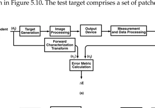
As with input devices, the calibration and characterization should then be evaluated with an independent test target. The flow diagram for doing this is shown in Figure 5.10. The test target comprises a set of patches with known

Device-independent data Device dependent

data GenerationTarget OutputDevice

Measurement and Data Processing Image Processing Device calibration, characterization {d }i {c }i Profile

Figure 5.9 Output device characterization workflow.

Device-dependent test data Target Generation Image Processing Output Device Forward Characterization Transform Error Metric Calculation ∆E (a) {d } {c } {c }` Device-independent test data Target Generation Error Metric Calculation ∆E (b) {c } Inverse Characterization Transform {c }` i i i i i Measurement and Data Processing

Image

Processing OutputDevice

Measurement and Data Processing

device-independent coordinates. If calibration is being tested, this target is processed through the calibration functions and rendered to the device. If characterization is being evaluated, the target is processed through both the characterization and calibration function and rendered to the device. The resulting output is measured in device-independent coordinates and com-pared with the original target values. Once again, the comparison is to be carried out with an appropriate color difference formula such as ∆ or ∆ . An important component of the color characteristics of an output device is its color gamut, namely the volume of colors in three-dimensional colori-metric space that is physically achievable by the device. Of particular impor-tance is the gamut surface, as this is used in gamut mapping algorithms. This information can easily be derived from the characterization process. Details of gamut surface calculation are provided in the chapter on gamut mapping.

5.3 Characterization targets and measurement techniques

5.3.1 Color target design

The design of a color target involves several factors. First is the set of colo-rants and underlying medium of the target. In the case of input devices, the characterization target is created offline (i.e., it is not part of the character-ization process) with colorants and media that are representative of what the device is likely to capture. For example, for scanner characterization, photographic and offset lithographic processes are commonly used to create targets on reflective or transmissive media. In the case of output devices, target generation is part of the characterization process and should be carried out using the same colorants and media that will be used for final color rendition.

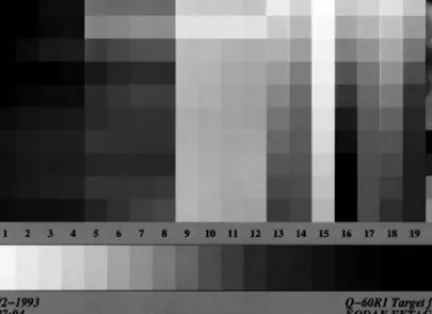
The second factor is the choice of color patches. Typically, the patches are chosen to span the desired range of the colors to be captured (in the case of input devices) or rendered (in the case of output devices). Often, critical memory colors are included, such as flesh tones and neutrals. The optimal choice of patches is logically a function of the particular algorithm or model that will be used to generate the calibration or characterization function. Nevertheless, a few targets have been adopted as industry stan-dards, and they accommodate a variety of characterization techniques. For input device characterization, these include the CGATS/ANSI IT8.7/1 and IT8.7/2 targets for transmission and reflection media respectively (http://webstore.ansi.org/ansidocstore); the Kodak photographic Q60 tar-get, which is based on the IT8 standards and is made with Ektachrome dyes on Ektacolor paper (www.kodak.com); the GretagMacbeth ColorChecker chart (www.munsell.com); and ColorChecker DC version for digital

cam-Eab

*

E94 *

eras (www.gretagmacbeth.com). For output device characterization, the common standard is the IT8.7/3 CMYK target (http://webstore.ansi.org/ ansidocstore). The Q60 and IT8.7/3 targets are shown in Plates 5A and 5B. A third factor is the spatial layout of the patches. If a device is known to exhibit spatial nonuniformity, it may be desirable to generate targets with the same set of color patches but rendered in different spatial layouts. The measurements from the multiple targets are then averaged to reduce the effect of the nonuniformity. In general, this approach is advised so as to reduce the overall effect of various imperfections and noise in the character-ization process. In the case of input devices, target creation is often not within the practitioner’s control; rather, the targets are supplied by a third-party vendor such as Eastman Kodak or Fuji Film. Generally, however, these vendors do use similar principles to generate reliable measurement data.

Another motivation for a specific spatial layout is visual inspection of the target. The Kodak Q60 target, for example, is designed with a gray ramp at the bottom and neutral colors all collected in one area. This allows for convenient visual inspection of these colors, to which we are more sensitive.

5.3.2 Color measurement techniques

5.3.2.1 Visual approaches

Most visual approaches rely on observers making color matching judgments. Typically, a varying stimulus produced by a given device is compared against a reference stimulus of known measurement. When a visual match is reported, this effectively provides a measurement for the varying stimulus and can be correlated with the device value that produced the stimulus. The major advantage of a visual approach is that it does not require expensive measurement instrumentation. Proponents also argue that the best color measurement device is the human visual system, because, after all, this is the basis for colorimetry. However, these approaches have their limitations. First, to achieve reliable results, the visual task must be easy to execute. This imposes severe limits on the number and nature of measurements that can be made. Second, observer-to-observer variation will produce measurements and a characterization that may not be satisfactory to all observers. Never-theless, visual techniques are appealing in cases where the characterization can be described by a simple model and thus derived with a few simple measurements. The most common application of visual approaches is thus found in CRT characterization, discussed further in Section 5.8.3.

5.3.2.2 Instrument-based approaches

Color measurement instruments fall into two general categories, broadband and narrowband. A broadband measurement instrument reports up to three color signals obtained by optically processing the input light through broad-band filters. Photometers are the simplest example, providing a measure-ment only of the luminance of a stimulus. Their primary use is in

determin-Chapter five: Device characterization 287

Figure 5A (See color insert following page 430) Q60 input characterization target.

ing the nonlinear calibration function of displays (discussed in Section 5.8). Densitometers are an example of broadband instruments that measure opti-cal density of light filtered through red, green, and blue filters. Colorimeters are another example of broadband instruments that directly report tristim-ulus (XYZ) values and their derivatives such as CIELAB. In the narrowband category fall instruments that report spectral data of dimensionality signif-icantly larger than three. Spectrophotometers and spectroradiometers are examples of narrowband instruments. These instruments typically record spectral reflectance and radiance, respectively, within the visible spectrum in increments ranging from 1 to 10 nm, resulting in 30 to 300 channels. They also have the ability to internally calculate and report tristimulus coordinates from the narrowband spectral data. Spectroradiometers can measure both emissive and reflective stimuli, while spectrophotometers can measure only reflective stimuli.

The main advantages of broadband instruments such as densitometers and colorimeters are that they are inexpensive and can read out data at very high rates. However, the resulting measurement is only an approximation of the true tristimulus signal, and the quality of this approximation varies widely, depending on the nature of the stimulus being measured. Accurate colorimetric measurement of arbitrary stimuli under arbitrary illumination and viewing conditions requires spectral measurements afforded by the more expensive narrowband instruments. Traditionally, the printing indus-try has satisfactorily relied on densitometers to make color measurements of prints made by offset ink. However, given the larger variety of colorants, printing technologies, and viewing conditions likely to be encountered in today’s digital color imaging business, the use of spectral measurement instruments is strongly recommended for device characterization. Fortu-nately, the steadily declining cost of spectral instrumentation makes this a realistic prospect.

Instruments measuring reflective or transmissive samples possess an internal light source that illuminates the sample. Common choices for sources are tungsten-halogen bulbs as well as xenon and pulsed-xenon sources. An important consideration in reflective color measurement is the optical geometry used to illuminate the sample and capture the reflected light. A common choice is the 45/0 geometry, shown in Figure 5.11. (The two numbers are the angles with respect to the surface normal of the incident illumination and detector respectively.) This geometry is intended to mini-mize the effect of specular reflection and is also fairly representative of the conditions under which reflection prints are viewed. Another consideration is the measurement aperture, typically set between 3 and 5 mm. Another feature, usually offered at extra cost with the spectrophotometer, is a filter that blocks out ultraviolet (UV) light emanated by the internal source. The filter serves to reduce the amount of fluorescence in the prints that is caused by the UV light. Before using such a filter, however, it must be remembered that common viewing environments are illuminated by light sources (e.g., sunlight, fluorescent lamps) that also exhibit a significant amount of UV

energy. Hence, blocking out UV energy may provide color measurements that are less germane to realistic viewing conditions.

For reflective targets, another important factor to consider is the color of the backing surface on which the target is placed for measurement. The two common options are black and white backing, both of which have advantages and disadvantages. A black backing will reduce the effect of show-through from the image on the backside of a duplex print. However, it will also expose variations in substrate transmittance, thus resulting in noisier measurements. A white backing, on the other hand, is not as effective at attenuating show-through; however, the resulting measurements are less noisy, because the effect of substrate variations is reduced. Generally, a white backing is recommended if the target is not duplex (which is typically the case.) Further details are provided by Rich.9

Color measurement instruments must themselves be calibrated to output reliable and repeatable data. Instrument calibration entails understanding and specifying many of the aforementioned parameters and, in some cases, needs to be carried out frequently. Details are provided by Zwinkel.10

Because color measurement can be a labor-intensive task, much has been done in the color management industry to automate this process. The Gretag SpectrolinoTM _{product enables the target to be placed on a stage and}

auto-matically measured by the instrument. These measurements are then stored on a computer to be retrieved for deriving the characterization. In a similar vein, X-Rite Corporation has developed the DTP-41 scanning spectropho-tometer. The target is placed within a slot in the “strip reader” and is auto-matically moved through the device as color measurements are made of each patch.

5.3.3 Absolute and relative colorimetry

An important concept that underlies device calibration and characterization is normalization of the measurement data by a reference white point. Recall from an earlier chapter that the computation of tristimulus XYZ values from spectral radiance data is given by

Sample

Illumination Detector and

Monochromator

45°

(5.9)

where = color matching functions V = set of visible wavelengths K = a normalization constant

In absolute colorimetry, K is a constant, expressed in terms of the maximum efficacy of radiant power, equal to 683 lumens/W. In relative colorimetry, K is chosen such that Y = 100 for a chosen reference white point.

(5.10)

where Sw(λ) = the spectral radiance of the reference white stimulus.

For reflective stimuli, radiance Sw(λ) is a product of incident illumination

I(λ) and spectral reflectance Rw(λ) of a white sample. The latter is usually

chosen to be a perfect diffuse reflector (i.e., Rw(λ) = 1) so that Sw(λ) = I(λ) in

Equation 5.10.

There is an additional white-point normalization to be considered. The conversion from tristimulus values to appearance coordinates such as CIELAB or CIELUV requires the measurement of a reference white stimulus and an appropriate scaling of all tristimulus values by this white point. In the case of emissive display devices, the white point is the measurement of the light emanated by the display device when the driving RGB signals are at their maximal values (e.g., DR = DG = DB = 255 for 8-bit input). In the case

of reflective samples, the white point is obtained by measuring the light emanating from a reference white sample illuminated by a specified light source. If an ideal diffuse reflector is used as the white sample, we refer to the measurements as being in media absolute colorimetric coordinates. If a par-ticular medium (e.g., paper) is used as the stimulus, we refer to the mea-surements as being in media relative colorimetric coordinates. Conversions between media absolute and relative colorimetry are achieved with a white-point normalization model such as the von Kries formula.

To get an intuitive understanding of the effect of media absolute vs. relative colorimetry, consider an example of scan-to-print reproduction of a color image. Suppose the image being scanned is a photograph whose medium typically exhibits a yellowish cast. This image is to be printed on a xerographic printer, which typically uses a paper with fluorescent whit-eners and is thus lighter and bluer than the photographic medium. The image is scanned, processed through both scanner and printer characteriza-tion funccharacteriza-tions, and printed. If the characterizacharacteriza-tions are built using media absolute colorimetry, the yellowish cast of the photographic medium is

X K S( )λ x( )∂λλ , Y λε

∫

∫

∫

∫

preserved in the xerographic reproduction. On the other hand, with media relative colorimetry, the “yellowish white” of the photographic medium maps directly to the “bluish white” of the xerographic medium under the premise that the human visual system adapts and perceives each medium as “white” when viewed in isolation. Arguments can be made for both modes, depending on the application. Side-by-side comparisons of original and reproduction may call for media absolute characterization. If the repro-duction is to be viewed in isolation, it is probably preferable to exploit visual white-point adaptation and employ relative colorimetry. To this end, the ICC specification supports both media absolute and media relative modes in its characterization tables.

Finally, we remark that, while a wide variety of standard illuminants can be selected for deriving the device characterization function, the most common choices are CIE daylight illuminants D5000 (typically used for reflection prints) and D6500 (typically used for the white point of displays).

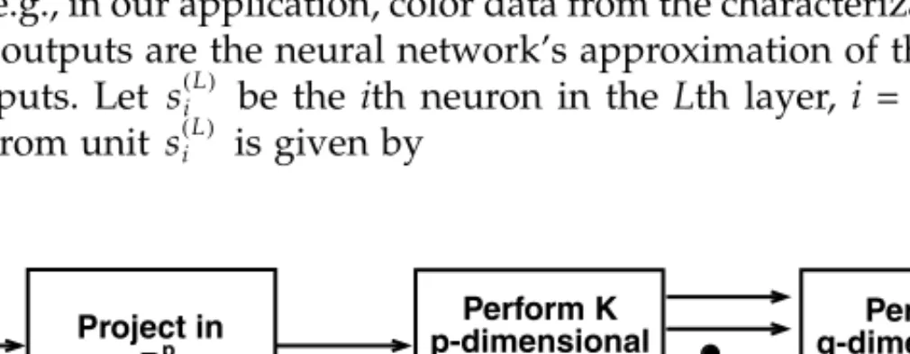
5.4 Multidimensional data fitting and interpolation

Generally, the data samples generated by the characterization process in both device-dependent and device-independent spaces will constitute only a small subset of all possible digital values that could be encountered in either space. One reason for this is that the total number of possible samples in a color space is usually prohibitively large for direct measurement of the characterization function. As an example, for R, G, B signals represented with 8-bit precision, the total number of possible colors is 224 _{= 16,777,216;}

clearly an unreasonable amount of data to be acquired manually. However, because the final characterization function will be used for transforming arbitrary image data, it needs to be defined for all possible inputs within some expected domain. To accomplish this, some form of data fitting or interpolation must be performed on the characterization samples. In model-based characterization, the underlying physical model serves to perform the fitting or interpolation for the forward characterization function. With empir-ical approaches, mathematempir-ical techniques may be used to perform data fitting or interpolation. Some of the common mathematical approaches are discussed in this section.

The fitting or interpolation concept can be formalized as follows. Define a set of T m-dimensional device-dependent color samples {di} ∈ Rm, i = 1,

. . ., T generated by the characterization process. Define the corresponding set of n-dimensional device-independent samples {ci} ∈ Rn, i = 1, . . ., T. For

the majority of characterization functions, n = 3, and m = 3 or 4. We will often refer to the pair ({di}, {ci}) as the set of training samples. From this set,

• f: F∈ Rm→ _Rn_{, mapping device-dependent data within a domain F}

to device-independent color space

• g: G∈ Rn→ _Rm_{, mapping device-independent data within a domain}

G to device-dependent color space

In interpolation schemes, the error of the functional approximation is identically zero at all the training samples, i.e., f(di) = ci, and g(ci) = di, i =

1, . . ., T.

In fitting schemes, this condition need not hold. Rather, the fitting func-tion is designed to minimize an error criterion between the training samples and the functional approximations at these samples. Formally,

(5.11) where E1 and E2 are suitably chosen error criteria.

A common approach is to pick a parametric form for f (or g) and mini-mize the mean squared error metric, given by

(5.12)

An analogous expression holds for E2. The minimization is performed with

respect to the parameters of the function f or g.

Unfortunately, most of the data fitting and interpolation approaches to be discussed shortly are too computationally expensive for the processing of large amounts of image pixel data in real time. The most common way to address this problem is to first evaluate the complex fitting or interpolation functions at a regular lattice of points in the input space and build a multi-dimensional lookup table (LUT). A fast interpolation technique such as tri-linear or tetrahedral interpolation is then used to transform image data using this LUT. The subject of fast LUT interpolation on regular lattices is treated in a later chapter. Here, we will focus on the fitting and interpolation methods used to initially approximate the characterization function and build the LUT. Often, it is necessary to evaluate the functions f and g within domains F

and G that are outside of the volumes spanned by the training data {di} and

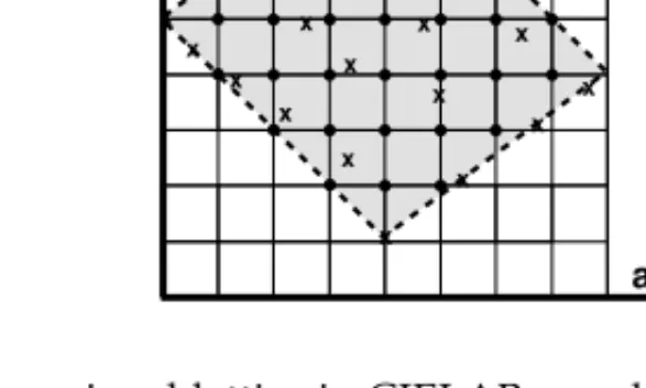
{ci}. An example is shown in Figure 5.12 for printer characterization mapping

CIELAB to CMY. A two-dimensional projection of CIELAB space is shown, with a set of training samples {ci} indicated by “x.” Device-dependent CMY

values {di} are known at each of these points. The shaded area enclosed by

these samples is the range of colors achievable by the printer, namely its color gamut. From these data, the inverse printer characterization function from CIELAB to CMY is to be evaluated at each of the lattice points lying on the three-dimensional lookup table grid (projected as a two-dimensional grid in

f

fopt= argminE1(ci,f( )di i=1,…,T); gopt= argminE2(di,g( )ci i=1,…,T)

g E1 1 T ---i=1 T

∑

Figure 5.12). Hence, the domain G in this case is the entire CIELAB cube. Observe that a fraction of these lattice points lie within the printer gamut (shown as black circles). Interpolation or data fitting of these points is usually well defined and mathematically robust, since a sufficient amount of training data is available in the vicinity of each lattice point. However, a substantial fraction of lattice points also lie outside the gamut, and there are no training samples in the vicinity of these points. One of two approaches can be used to determine the characterization function at these points.

1. Apply a preprocessing step that first maps all out-of-gamut colors to the gamut, then perform data fitting or interpolation to estimate output values.

2. Extrapolate the fitting or interpolation function to these out-of-gamut regions.

Some of the techniques described herewith allow for data extrapolation. The latter will invariably generate output data that lie outside the allowable range in the output space. Hence, some additional processing is needed to limit the data to this range. Often, a hard-limiting or clipping function is employed to each of the components of the output data.

Two additional comments are noteworthy. First, while the techniques described in this section focus on fitting and interpolation of multidimen-sional data, most of them apply in a straightforward manner to one-dimen-sional data typically encountered in device calibration. Linear and polyno-mial regression and splines are especially popular choices for fitting one-dimensional data. Lattice-based interpolation reduces trivially to piecewise linear interpolation, and it can be used when the data are well behaved and exhibit low noise. Secondly, the reader is strongly encouraged, where pos-sible, to plot the raw data along with the fitting or interpolation function to obtain insight on both the characteristics of the data and the functional approximation. Often, data fitting involves a delicate balance between accu-rately approximating the function and smoothing out the noise. This balance

a* L* lookup table lattice x x x x x x x x x x x x x x x x x x x x x x printer gamut x

294 Digital Color Imaging Handbook is difficult to achieve by examining only a single numerical error metric and is significantly aided by visualizing the entire dataset in combination with the fitting functions.

5.4.1 Linear least-squares regression

This very common data fitting approach is used widely in color imaging, particularly in device characterization and modeling. The problem is formu-lated as follows. Denote d and c to be the input and output color vectors, respectively, for a characterization function. Specifically, d is a 1 ¥m vector, and c is a 1 ¥n vector. We wish to approximate the characterization function by the linear relationship c = d · A.

The matrix A is of dimension m¥n and is derived by minimizing the mean squared error of the linear fit to a set of training samples, {di, ci}, i =

1, . . ., T. Mathematically, the optimal A is given by

(5.13) To continue the formulation, it is convenient to collect the samples {ci} into

a T¥n matrix C = [c1, . . ., cT], and {di} into a T¥m matrix D = [d1, . . ., dT].

The linear relationship is given by C = D · A. The optimal A is given by A = D† C, where D† is the generalized inverse (sometimes known as the Moore–Penrose pseudo-inverse) of D. In the case where Dt_{D is invertible,}

the optimum A is given by

A = (Dt_D)–1_Dt_{C (5.14)}

See Appendix 5.A for the derivation and numerical computation of this least-squares solution. It is important to understand the conditions for which the solution to Equation 5.14 exists. If T < m, we have an underdetermined system of equations with no unique solution. The mathematical consequence of this is that the matrix Dt_{D is of insufficient rank and is thus not invertible.}

Thus, we need at least as many samples as the dimensionality of the input data. If T = m, we have an exact solution for A that results in the squared error metric being identically zero. If T > m (the preferred case), Equation 5.14 provides a least-squares solution to an overdetermined system of equa-tions. Note that linear regression affords a natural means of extrapolation for input data d lying outside the domain of the training samples. As men-tioned earlier, some form of clipping will be needed to limit such extrapo-lated outputs to their allowable range.

5.4.2 Weighted least-squares regression

The standard least-squares regression can be extended to minimize a weighted error criterion,

A Aopt argmin 1

T ---i=1 T

Â

(5.15)

where wi = positive-valued weights that indicate the relative importance

of the ith data point, {di, ci}.

Adopting the notation in Section 5.4.1, a straightforward extension of Appen-dix 5.A results in the following optimum solution:

A = (Dt_WD)–1_Dt_{WC (5.16)}

where W is a T × T diagonal matrix with diagonal entries wi.

The resulting fit will be biased toward achieving greater accuracy at the more heavily weighted samples. This can be a useful feature in device char-acterization when, for example, we wish to assign greater importance to colors in certain regions of color space (e.g., neutrals, fleshtones, etc.). As another example, in spectral regression, it may be desirable to assign greater importance to certain wavelengths than others.

5.4.3 Polynomial regression

This is a special form of least-squares fitting wherein the characterization function is approximated by a polynomial. We will describe the formulation using, as an example, a scanner characterization mapping device RGB space to XYZ tristimulus space. The formulation is conceptually identical for input and output devices and for the forward and inverse functions.

The third-order polynomial approximation for a transformation from RGB to XYZ space is given by

(5.17) where wX,l, etc. = polynomial weights

l = a unique index for each combination of i, j, k

In practice, several of the terms in Equation 5.17 are eliminated (i.e., the weights w are set to zero) so as to control the number of degrees of freedom in the polynomial. Two common examples, a linear and third-order approximation,

Aopt argmin

1 T --- wi ci–diA 2 i=1 T

∑

∑

∑

∑

∑

∑

∑

∑

∑

∑

are given below. For brevity, only the X term is defined; analogous definitions hold for Y and Z.

X = wX,0R + wX,1G + wX,2B (5.18a)

X = wX,0 + wX,1R + wX,2G + wX,3B + wX,4RG + wX,5GB

+ wX,6RB + wX,7R2 + wX,8G2 + wX,9B2 + wX,10RGB (5.18b)

In matrix-vector notation, Equation 5.17 can be written as

(5.19)

or more compactly,

c = p · A (5.20)

where c = output XYZ vector

p = 1 ×Q vector of Q polynomial terms derived from the input RGB vector d

A =Q ×3 matrix of polynomial weights to be optimized

In the complete form, Q = 64. However, with the more common simplified approximations in Equation 5.18, this number is significantly smaller; i.e., Q = 3 and Q = 11, respectively.

Note from Equation 5.20 that the polynomial regression problem has been cast into a linear least-squares problem with suitable preprocessing of the input data d into the polynomial vector p. The optimal A is now given by

(5.21) Collecting the samples {ci} into a T × 3 matrix C = [c1, . . ., cT], and {pi} into

a T × Q matrix P = [p1, . . ., pT], we have the relationship C = P · A. Following

the formulation in Section 5.4.1, the optimal solution for A is given by

A = (Pt_P)–1_Pt_{C (5.22)}

For the Q ×Q matrix (Pt_{P) to be invertible, we now require that T} ≥ _Q.

X Y Z 1R G … R3G3B3 wX,0 wY,0 wZ,0 wX,1 wY,1 wz,3 … wX,63 wY,63 wZ,63 =

Aopt argmin

1 T --- ci–piA 2 i=1 T

∑

Polynomial regression can be summarized as follows:

1. Select a set of T training samples, where T > Q, the number of terms in the polynomial approximation. It is recommended that the sam-ples adequately span the input color space.

2. Use the assumed polynomial model to generate the polynomial terms

pi from the input data di. Collect ci and pi into matrices C and P,

respectively.

3. Use Equation (5.22 to derive the optimal A.

4. For a given input color d, use the same polynomial model to generate the polynomial terms p.

5. Use Equation 5.20 to compute the output color c.

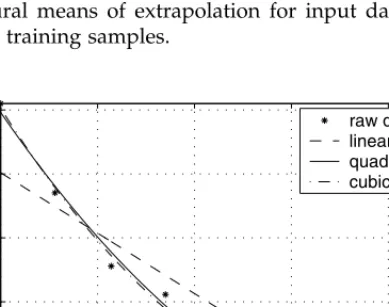
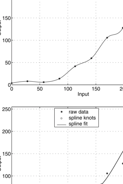
Figure 5.13 is a graphical one-dimensional example of different polynomial approximations to a set of training samples. The straight line is a linear fit (Q = 3) and is clearly inadequate for the given data. The solid curve is a second-order polynomial function (Q = 7) and offers a much superior fit. The dash–dot curve closely following the solid curve is a third-order poly-nomial approximation (Q = 11). Clearly, this offers no significant advantage over the second-order polynomial. In general, we recommend using the smallest number of polynomial terms that adequately fits the curvature of the function while still smoothing out the noise. This choice is dependent on the particular device characteristics and is obtained by experimentation, intuition, and experience. Finally, it is noted that polynomial regression affords a natural means of extrapolation for input data lying outside the domain of the training samples.

0 50 100 150 200 250 50 0 50 100 150 200 250

Cyan digital count

Luminance

raw data linear fit quadratic fit cubic fit

5.4.4 Distance-weighted techniques

The previous section described the use of a global polynomial function that results in the best overall fit to the training samples. In this section, we describe a class of techniques that also employ simple parametric functions; however, the parameters vary across color space to best fit the local charac-teristics of the training samples.

5.4.4.1 Shepard’s interpolation

This is a technique that can be applied to cases in which the input and output spaces of the characterization function are of the same dimensionality. First, a crude approximation of the characterization function is defined: = fapprox(d). The main purpose of fapprox() is to bring the input data into the

orientation of the output color space. (By “orientation,” it is meant that all RGB spaces are of the same orientation, as are all luminance–chrominance spaces, etc.) If both color spaces are already of the same orientation, e.g., printer RGB and sRGB, we can simply let fapprox() be an identity function so

that = d. If, for example, the input and output spaces are scanner RGB and CIELAB, an analytic transformation from any colorimetric RGB (e.g., sRGB) to CIELAB could serve as the crude approximation.

Next, given the training samples {di} and {ci} in the input and output

space, respectively, we define error vectors between the crude approximation and true output values of these samples: . Shepard’s interpolation for an arbitrary input color vector d is then given by11

(5.23)

where w() = weights

Kw = a normalizing factor that ensures that these weights sum to

unity as follows:

(5.24)

The second term in Equation 5.23 is a correction for the residual error between c and , and it is given by a weighted average of the error vectors

ei at the training samples. The weighting function w() is chosen to be

inversely proportional to the Euclidean distance between d and di so that

training samples that are nearer the input point exhibit a stronger influence than those that are further away. There are numerous candidates for w(). One form that has been successfully used for printer and scanner character-ization is given by12 cˆ cˆ ei = ci–cˆi, = 1, …,T c=cˆ Kw w(d–di) i=1 T

∑

∑

(5.25)

where denotes Euclidean distance between vectors d and di, and ρ

and ε are parameters that dictate the relative influence of the training samples as a function of their distance from the input point. As ρ increases, the influence of a training sample decays more rapidly as a function of its distance from the input point. As ε increases, the weights become less sen-sitive to distance, and the approach migrates from a local to a global approx-imation.

Note that, in the special case where ε = 0, the function in Equation 5.25 has a singularity at d = di. This can be accommodated by adding a special

condition to Equation 5.23.

(5.26)

where w() = given by Equation 5.25 with ε = 0

t = a suitably chosen distance threshold that avoids the singularity at d = di

Other choices of w() include the Gaussian and exponential functions.11 _Note

that, depending on how the weights are chosen, Shepard’s algorithm can be used for both data fitting (i.e., Equation 5.23 and Equation 5.25 with ε > 0), and data interpolation, wherein the characterization function coincides exactly at the training samples (i.e., Equation 5.26). Note also that this tech-nique allows for data extrapolation. As one moves farther away from the volume spanned by the training samples, the distances and hence the weights w() approach a constant. In the limit, the overall error correction in Equation 5.23 is an unweighted average of the error vectors ei.

5.4.4.2 Local linear regression

In this approach, the form of the characterization function that maps input colors d to output colors c is given by

c = d · Ad (5.27)

This looks very similar to the standard linear transformation, the important difference being that the matrix Ad now varies as a function of the input color d (hence the term local linear regression). The optimal Ad is obtained by a distance-weighted least-squares regression,

w(d–di) 1 d–di p ε + ---= d–di c cˆ Kw w(d–di)ei i=1 T

∑

(5.28)

As with Shepard’s interpolation, the weighting function w() is inversely proportional to the Euclidean distance , so training samples di that

are farther away from the input point d are assigned a smaller weight than nearby points. A form such as Equation 5.25 may be used.12 _{The solution is}

given by Equation 5.16 in Section 4.2, where the weights w(d – di) constitute

the diagonal terms of W. Note that because w() is a function of the input vector d, Equation 5.16 must be recalculated for every input vector d. Hence, this is a computationally intensive algorithm. Fortunately, as noted earlier, this type of data fitting is not applied to image pixels in real time. Instead, it is used offline to create a multidimensional lookup table.

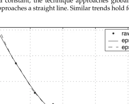
Figure 5.14 is a one-dimensional example of the locally linear transform using the inverse-distance weighting function, Equation 5.25. As with Shep-ard’s interpolation, ρ and ε affect the relative influence of the training sam-ples as a function of distance. The plots in Figure 5.14 were generated with

ρ = 4 and compare two values of ε. For ε = 0.001, the function closely follows the data. As ε increases to 0.01, the fit averages the fine detail while preserv-ing the gross curvature. In the limit as ε increases, w() in Equation 5.25 approaches a constant, the technique approaches global linear regression, and the fit approaches a straight line. Similar trends hold for ρ. These

param-Ad opt min arg 1 T ---