NATIONAL INSTITUTE OF TECHNOLOGY , ROURKELA
Solving Target Coverage Problem in
Wireless Sensor Networks Using
Iterative Heuristic Algorithms
by
Akansha
A thesis submitted in partial fulfillment for the degree of Bachelor of Technology
under the supervision of
Prof. Bibhudatta Sahoo Computer Science and Engineering
Certificate
04 May, 2015
This is to certify that the work in the thesis entitledSolving Target Coverage Prob-lem in Wireless Sensor Networks Using Iterative Heuristic Algorithms by
Akansha, bearing Roll No. 111CS0113,, is a record of an original research work carried out by her under my supervision and guidance in partial fulfillment of the requisites for the award of the degree of Bachelor of Technology in Computer Science and Engineering. Neither this thesis nor any part of it has been submitted for any degree or academic award elsewhere.
Prof. Bibhudatta Sahoo
Dept. of Computer Science and Engineering National Institute of Technology Rourkela - 769008
.
Abstract
Wireless Sensor Networks have proved to be very useful in monitoring environmental conditions of remote or inhospitable areas. One of the major difficulty which a designer faces in devising such wireless sensor networks is the limited energy and computational resources available to sensor nodes of the networks. Thus, any application developed at any level of hierarchy must be designed keeping in mind its constraints.
The first work in establishing a sensor network is the deployment of sensor nodes .one solution in case of deployment of sensor nodes in an inhospitable area in which ground access is prohibited is to drop the sensor nodes from aircraft. Since the exact positioning of the sensor nodes on the ground cannot be guaranteed , one solution is to deploy a large number of nodes. Therefore, the number of nodes that are deployed ,with an aim to cover the area completely, is often higher than the required. Activating only those nodes that are necessary at any particular moment rather than all the sensor nodes can save energy. Hence, we divide the sensor nodes into sets such that each set is capable of monitoring all targets and activate those sets one after another. So the overall all lifetime of WSNs will be the sum of the lifetime of cover sets.This process will effectively lead to increment in the overall lifetime of WSN.
This work aims to maximize the lifetime of wireless sensor networks by grouping the sensor nodes into sets and activating the sets successively.By lifetime is meant the to-tal time for which the sensor nodes can monitor the whole target area or all the target objects. Two different cases have been dealt with- one when the transmission and recep-tion range of sensors can be adjusted and the other in which the range of transmission and reception is fixed.Three different algorithmic paradigms are used- Greedy heuristic ,Genetic Algorithm and Particle Swarm Optimization.
Acknowledgements
.It had been a long time for me when I started this work and now when I am writing this, I am going to take the privilege of thanking all those people who have helped me to put all the ideas and work, well above the level of simplicity and into something concrete.
I thank whole heartedly, Prof.B.D Sahoo for making me a part of this valuable project, constantly motivating me for doing better and showing complete confidence in my work . As my supervisor, he has extended appropriate help at every point which has proved very relevant in understanding the problem area and working on the solution.In addition his constant encouragement,observations and comments have helped me to follow the right direction in the research and to move forward with an investigation in depth. He has helped me greatly and been a source of knowledge.Also in the process, I learnt a lot other technical and non-technical things from him.
I must acknowledge all the help in form of academic or non-academic resources that I have got from my institute NIT Rourkela. I would like to thank all the administrative and technical staff members of the Department who has been kind enough to advise and assist in their respective roles.
Last, but not the least, I would like to thanks my friends for motivating me and dis-cussing all technical stuffs. I would like to dedicate this thesis to my parents,sister and brother, for their love, patience, and understanding.
Contents
Certificate i Abstract ii Acknowledgements iii List of Figures v List of Tables vi 1 Introduction 1 1.1 Motivation . . . 2 1.2 Problem Background . . . 41.3 Research Statement with Research Questions . . . 5
1.4 Goal of the Research . . . 6
1.5 Scope of the study . . . 6
1.6 Thesis Outline . . . 7
2 The Target Coverage Problem 9 2.1 An example of WSN With 3 Targets and 4 Sensors . . . 11
2.2 The scheduling mechanism. . . 12
2.3 NP-Completeness . . . 13
2.4 Literature Review . . . 13
2.5 SENSOR DEPLOYMENT. . . 15
2.5.1 Deployment Technique . . . 15
2.5.2 RESULTS . . . 17
3 Nodes with Fixed Range 29 3.1 Assumptions . . . 29
3.2 Problem Statement . . . 30
3.3 Greedy MSC Algorithm . . . 30
3.4 Proposed greedy algorithm . . . 33
4 Sensor Nodes with Adjustable Ranges 36 4.1 Assumtion . . . 36 4.2 Problem Statement . . . 37 4.3 Problem scenario . . . 37 4.4 ARSC Algorithm . . . 40 4.5 Simulation results . . . 43
5 Genetic Algorithm and Particle Swarm Optimization 44 5.1 Genetic Algorithm Overview . . . 44
5.2 Assumtion . . . 47 5.3 Problem Statement . . . 47 5.4 Implementation Details . . . 47 5.4.1 Chromosome Structure . . . 48 5.4.2 Cost Function. . . 48 5.4.3 Selection Operator . . . 49 5.4.4 Crossover Operator. . . 49 5.4.5 Mutation Operator . . . 50
5.5 The Genetic Algorithm . . . 50
5.6 Simulation Results . . . 53
5.7 Particle Swarm Optimization . . . 54
5.8 Overview of Particle Swarm Optimization Algorithm . . . 55
5.9 Implementation details . . . 56
5.9.1 Particle Structure . . . 56
5.9.2 Cost Function. . . 56
5.10 Comparision of Genetic Algorithm and Particle Swarm Optimization Al-gorithm . . . 57
5.11 PSO algorithm . . . 58
5.12 Simulation Result. . . 60
A Appendix Title Here 62
List of Figures
2.1 A WSN With 3 Targets and 4 Sensors . . . 11
2.2 S1=s3,s4 for 1s . . . 11 2.3 S1=s1,s2 for 1s . . . 11 2.4 S1=s1,s2 for 0.5s . . . 12 2.5 S2=s4 for 1s. . . 12 2.6 S3=s1,s3 for 0.5s . . . 12 2.7 S4=s2,s3 for 0.5s . . . 12 2.8 CASE I . . . 18
2.9 CASE II:EFFECT OF INCREASE IN TRANSMISSION RANGE . . . . 19
2.10 CASE III:Effect of increase in nodes . . . 20
2.11 Deployment graph with n=20 . . . 20
2.12 Deployment graph with n=30 . . . 20
2.13 Deployment graph with n=40 . . . 21
2.14 Deployment graph with n=50 . . . 21
2.15 Deployment graph with n=60 . . . 21
2.16 Deployment graph with n=70 . . . 21
2.17 Deployment graph with n=80 . . . 22
2.18 Deployment graph with n=90 . . . 22
2.19 Deployment graph with n=30 . . . 23
2.20 Deployment graph with n=40 . . . 23
2.21 Deployment graph with n=50 . . . 23
2.22 Deployment graph with n=60 . . . 23
2.23 Deployment graph with n=70 . . . 24
2.24 Deployment graph with n=80 . . . 24
2.25 Deployment graph with n=90 . . . 24
2.26 Deployment graph with n=100 . . . 24
2.27 Deployment graph with n=30 . . . 25
2.28 Deployment graph with n=40 . . . 25
2.29 Deployment graph with n=50 . . . 26
2.30 Deployment graph with n=60 . . . 26
2.31 Deployment graph with n=70 . . . 26
2.32 Deployment graph with n=80 . . . 26
2.33 Deployment graph with n=90 . . . 27
2.34 Deployment graph with n=100 . . . 27
2.35 Deployment graph with n=110 . . . 27
4.1 WSN consisting of 3 targets and four sensors with 2 sensing ranges . . . 38
4.2 WSN consisting of 3 targets and four sensors with 2 sensing ranges . . . 38
4.3 { . . . 39
4.4 C2={(S4,R1),(S2,R2)} . . . 39
4.5 C3={(S4,R1) ,(S3,R2)} . . . 39
4.6 C1={S1} . . . 40
4.7 C2={S2,S4} . . . 40
4.8 Result of ARSC and FRSC algorithm . . . 43
5.1 An example of chromosome structure. . . 48
5.2 An example of single point crossover . . . 49
5.3 An example of single point crossover . . . 50
5.4 Result of GA algorithm with five and ten targets . . . 53
5.5 Result of GA algorithm with 15 and 20 targets . . . 53
5.6 Result of GA algorithm with 25 and 30 targets . . . 53
5.7 Result of GA algorithm with 35 and 40 targets . . . 54
5.8 An example of particle structure . . . 57
5.9 Result of PSO algorithm with five and ten targets . . . 60
5.10 Result of PSO algorithm with 15 and 20 targets. . . 61
5.11 Result of PSO algorithm with 25 and 30 targets. . . 61
List of Tables
Chapter 1
Introduction
A wireless sensor network (WSN) consists of autonomous sensor nodes deployed in an area to monitor physical and environmental conditions, such as tempera-ture, sound,pressure, etc.The information collected by individual sensor nodes are passed on to asink node where all these information are processed and some in-sight into the environmental conditions of the place of deployment of WSNs is gained.There are several keycomponents of a Wireless Sensor Networks which are as
followed:-• Low-power embedded processor:Low embedded processor is responsible for performing all the computational works in particular , processing of local information and transmission of information to other sensor nodes.Because of high cost , these are significantly constrained in terms of computational power.
• Memory/Storage: Program and data memory are stored on Random Access Memory or Read Only Memory.
• Radio transceiver: WSN devices include a low-rate, short-range wireless radio (10-100kbps, 100 m). Sensor nodes: Sensor nodes are the central component of WSNs. There are many types of sensors such temperature sensors, light
chemical sensors, acoustic sensors.The specific sensor used in a WSN is de-pends on the application.
• Geopositioning system: It is used to mark the location of sensor nodes which is useful in some applications.
• Power source: Due to physical and other constraints, WSN device is likely to be battery powered(e.g. using LiMH AA batteries).[6]
.Although WSNs are becoming increasingly popular for environmental monitoring ,it has certain constraints as well. Due to the small size of sensor nodes, the size of battery is also limited.And since the manual replacement of battery is not possible in many cases, the major constraint is the limited battery power A typical alkaline battery, for example, provides about 50 watt-hours of energy; this may prove to be operational for less than a month of continuous operation for each node in active mode [6].One of the main difficulties in the use of WSNs is how to use the battery efficiently.This is an optimization problem and many exact and approximate optimization algorithms have been applied to solve this problem .Still finding an optimal solution to this problem is an open challenge.In this thesis solution to the above-mentioned problem has been proposed by exact approximation algorithm i.e. greedy algorithm and some meta-heuristic algorithms such as Genetic Algorithm and Particle Swarm Optimization
1.1
Motivation
Wireless sensor networks promise an unheard, unexpected fine-grained interface between the virtual and physical worlds[1]. They are one of the most rapidly ad-vancing area of technology.They have applications in various areas such as indus-trial process ,environmental sensing, national security and surveillance, and struc-tural health monitoring. Recent improvements in cost of efficient electronic devices
3
have a considerable impact on advancing wireless sensor networks [2] . They repre-sent a smooth and convenient shift from traditional inter-human personal commu-nications to autonomous inter-device commucommu-nications.[1] They promise unprece-dented new abilities to observe and understand large-scale,real-world phenomena very minutely, at a fine spatio-temporal resolution.[1] As a result, wireless sen-sor networks also have the potential to give rise to new breakthrough scientific advancements[1].
As already mentioned ,the most important and critical aspect of wireless sen-sor networks is network lifetime that in turn depends on the lifetime of batter-ies of sensor nodes.Unlike conventional devices of everyday life such as mobile phones,palmtops, laptops etc that enjoy constant focus and attention by humans, the large scale of a wireless sensor network makes manual replenishment of energy impossible.[1] They are power-constrained and can be used as long as all the nodes are capable of sensing,transmitting and receiving.The size and weight of battery play a critical role in deciding the lifetime of the battery [1]. Since it may be un-feasible and expensive to replace the batteries of nodes of such large networks ,this calls for the need of utilizing the battery power judiciously so that they can re-main operational for a much longer period without any human intervention. This step can be taken at various levels such as hardware and architectural design and while developing algorithms and protocols at every layer of network architecture. An efficient and optimal algorithm that can extend the lifetime of the WSNs by judiciously utilizing battery power of the nodes is the need of the hour.
Classification of power preserving methods can be done as follows: [2]
• scheduling of the wireless nodes to switch from active state to sleep state and vice-versa to save energy
• adjustment of transmission range of wireless nodes to control power
• energy efficient routing, data gathering
• reduction of the amount of data transmitted and avoidance of useless activ-ities.
Here we will focus on the first method, that is, we design scheduling mechanism for saving power.
In our case, we are dealing with a case in which an area consisting of targets in which ground access is prohibited is given.The location of targets to be moni-tored is known.In order to monitor those targets, a large number of battery-driven sensor nodes have to be deployed and operated in an energy efficient way. The Range of the sensor can be uniform or varying depending upon the situation. Each sensor node has three operation modes: sensing, sleeping, and relaying.
1.2
Problem Background
There are many scenarios in which WSNs can be used.One particular situation that we are considering is described as follows: A remote area consisting of a set of targets to be monitored in which ground access is prohibited is given.We need to deploy sensors in that area.One solution to such problem is to drop the sensors from an aircraft. In that case ,it would not be possible to deploy the nodes at the exact position in the vicinity of the targets to be monitored in the given area.This problem of lack of precise positioning of the sensors can be tackled by deploying a large number of sensors.The presence of sensors in a number that is much greater than what is required can improve the probability of covering all the targets.In that case, we will have a large number of redundant sensors.
5
of sets such that each and every set can monitor all the targets. Then these sets can then be activated one after the other such that the lifetime of all cover sets will add up to extend the total lifetime of the sensor networks.Only the sensors of currently active set are responsible for monitoring all targets and for transmitting the data collected while all the other nodes are in a low-energy sleep mode. In this thesis ,we propose efficient iterative heuristic algorithms to extend the total lifetime of sensor network which work on the principle of organization of sensors nodes into maximum number of set covers which are activated one by one.
We design two iterative heuristics that efficiently frame the sets, using exact ap-proximation algorithm greedy heuristic and meta-heuristic algorithms such as ge-netic algorithm and Particle Swarm Optimization.
1.3
Research Statement with Research Questions
The above problem has been proved to be np-complete.We cannot find a poly-nomial time algorithm for this problem.So finding an optimal solution to this problem is an open challenge. Researchers have tried some traditional optimiza-tion algorithms such as greedy algorithm,branch and bound,linear programming, etc.However, they have shown excellent performance in addressing the problem, and there is still room for improvement.Moreover in most of the cases,they are not scalable to large networks as the runtime increases rapidly with an increase in the size of networks. Therefore, utilizing approximate algorithms like meta-heuristic algorithms in this regard, opens a new research area.
Artificial Immune System (AIS) , Genetic Algorithm, Ant Colony Optimization (ACO) ,Particle Swarm Optimization (PSO) , Artificial Bee Colony (ABC) , Im-perialistic Competitive Algorithm (ICA) are samples of meta-heuristic algorithms.
Therefore, more works are still required to develop the performance of exact ap-proximation algorithm and meta-heuristic algorithms to increase the lifetime of WSNs. Hence, new greedy algorithm and meta-heuristic algorithms are intro-duced to solve this problem.
Consequently, based on the above issues, the central research question is:
Are the proposed greedy and meta-heuristic algorithms beneficial in increasing the lifetime of WSNs as compared to already proposed algorithms?
Thus, the following issues need to be addressed:
• Could the proposed greedy algorithms be improved to increase the lifetime of WSNs?
• Since meta-heuristic algorithms are new research area, can any such algo-rithm be introduced to solve the problem efficiently?
• Could meta-heuristic algorithms perform better than traditional optimiza-tion greedy algorithm?
1.4
Goal of the Research
The goal of the research is to propose an improved greedy heuristic and a new meta-heuristic Particle Swarm Optimization (PSO) algorithm to increase the lifetime the sensor network by organizing the sensors into a maximal number of set covers that are activated successively.
7
1.5
Scope of the study
Recent technological advances allow us to view a future where a large numbers of low-power and inexpensive sensor devices are densely deployed in the physical en-vironment, working together in a wireless network.[1] The envisioned applications of these wireless sensor networks range widely from one field to another. Some of them are:[1]
• Monitoring of Ecological habitat
• Target tracking and military surveillance
• Seismic and structural monitoring
• Industrial and commercial networked sensing
The finite and limited battery energy is likely to be the most critical resource bottleneck in designing most of the WSN applications.This is the reason that when WSNs are designed, energy efficiency is kept as the primary goal. With such a broad scope of WSNs in future , one can understand the importance and scope of this study which deals with one of the most important and critical aspects of the WSNs i.e. extending the lifetime of WSNs.
1.6
Thesis Outline
A brief introduction of wireless sensor nodes ,motivation,problem background, research statement with the research question ,goal and scope of the study are presented in chapter 1.The rest of the thesis is organized into five chapters.
Chapter 2-This chapter deals with the scheduling mechanism.A real life example is presented and shown how scheduling helps in increasing the lifetime of WSN. A literature review is presented.Finally, deployment algorithm is given.Results are
Chapter 3-This chapter introduces the problem scenario of increasing the lifetime of WSN when the nodes have fixed range of transmission.The problem statement is presented .Greedy MSC algorithm has been implemented, and a new greedy heuristic has been proposed.Finally, the result of both the algorithms is presented
Chapter 4- This chapter introduces the problem scenario of increasing the life-time of WSN when the nodes have a variable range of transmission. The problem statement is presented, and ARSC algorithm is applied to solve the problem.The result of two algorithms has been compared - MSC algorithm presented in Chapter 3 and ARSC algorithm presented earlier in this chapter.
Chapter 5-In this chapter two meta-heuristic algorithm has been introduced-genetic algorithm and PSO.A introduced-genetic algorithm has been implemented, and a PSO algorithm has been proposed.The results of both the algorithm have been presented.
Chapter 2
The Target Coverage Problem
Our problem scenario can be described as follows - A remote area consisting of a set of targets to be monitored in which ground access is prohibited is given. We need to place the sensors randomly in the area keeping in mind the situation that sensor nodes are being dropped from an aircraft because of the prohibition of ground access to the area.In that case, it would not be possible to deploy the nodes at the exact position in the vicinity of the targets to be monitored in the given area.This problem of lack of accurate positioning of the Sensors can be tackled by deploying a large number of sensors.The presence of sensors in a number that is much greater than what is required can improve the probability of covering all the targets.In that case, we will have a large number of redundant sensors.Instead of activating all the sensors at a time, sensors can be divided into some sets.These sets are formed such that each can monitor all the targets.These sets can then be activated one after the another such that the lifetime of all cover sets will add up to extend the total lifetime of the sensor networks.Only the sensors from the current active set are incharge of supervision all the targets and for transmission of collected data, while all other nodes are kept in sleep mode, that is, a low-energy mode .[2]
sensor and the target is smaller or equal to the predefined sensing range , we will have a set of targets within the sensing range of every sensors.We need to frame cover sets consisting of a subset of sensor nodes such that each and every cover set can monitor all the targets.Only the sensor nodes from the current cover set will be activated, and the rest will be kept in low power state.The total lifetime of the network will then be defined as the summation of the lifetime of all the cover sets.Our goal is to maximize the lifetime of WSNs. Keeping only some nodes ac-tive at any time and rest in low power state can eventually lead to increment in the lifetime of the WSNs.Following are some of the studies regarding the energy requirement of sensors that can prove useful in our
problem:-• There are four different states in which radio of a sensor node can be: trans-mit, receive, sleep, or idle.Minimum energy is used when a sensor node is in sleep mode i.e. the radio of node is turned off.
• Power usage analysis of WINS Rockwell seismic sensor was carried out to get an idea of energy requirement in different modes of sensor nodes .The results drawn were power consumption for the transmit state was between 0.38W and O.7 W, 0.36W when in receive mode, 0.34W when in idle mode and for the sleep mode 0.03W. The energy requirements of the receive and idle modes may be as similar to that of transmission mode while the sleep mode requires less energy.
• Another observation is the ratio of communication to computation power us-age for Rockwell WINS is from 1500 to 2700; therefore data compression,local data processing, and data fusion are worthy.[2]
Hence, Lifetime can be extended by grouping sensor nodes into a number of sets such that each set covers all the targets and activating them successively.An ex-ample will further make it clear.
11
2.1
An example of WSN With 3 Targets and 4 Sensors
[2]
Figure 2.1: Three targets R=r1,r2,r3 and 4 sensors S=s1,s2,s3,s4
Forming set covers-1
Forming set covers-2
Figure 2.4: S1=s1,s2 for 0.5s Figure 2.5: S2=s4 for 1s
Figure 2.6: S3=s1,s3 for 0.5s
Figure 2.7: S4=s2,s3 for 0.5s
Total lifetime in 1st scenario is 1+1=2s .Total lifetime in second scenario is 0.5+1+0.5+0.5=2.5s. Lifetime in 2nd scenario is 25% more than the 1st scenario.This indicates that proper organization can increase the lifetime.
2.2
The scheduling mechanism
To design such a mechanism, we need to have some information such as when and how to decide for each node when to enter in sleep mode and for how much time. The steps
are:-• Location information are sent by sensor nodes to sink node
• Sensor scheduling algorithms are executed by the sink node and the schedule is broadcast when all nodes are active.
13
One another advantage is that the contention at MAC sublayer is also reduced. [2] .
2.3
NP-Completeness
This problem has been proved to be NP-Complete in [2].We cannot find a polynomial-time algorithm for solving it exactly. Hence finding an optimal solution to this problem is an open challenge. Researchers have proposed many heuristics that finds sub-optimal solution to the problem of finding maximal number of cover
sets:-• Linear programming
• Greedy
• Approximation
• Metaheuristic algorithms
• Branch and bound
In this thesis, we will solve the problem using greedy and meta-heuristic algo-rithms.
2.4
Literature Review
Sl.No Title/Author/ Year Time-Complexity
Objective Input Output Target distri-bution mode Greedy Heuris-tic 1 Energy-Efficient Target Coverage in Wire-less Sensor Network-sAuthors : M Cardei, M.T Thai, Y Li, W WuYear - 2005 O(im2n) Homogeneous Maxi-mum Set Cover Problem Set of Sensors n Set of targets R Compute Maxi-mum Set Covers Random Distri-bution Sensors with greatest contri-bution 2 High-Energy-First(HEF) Heuristic for Energy-Efficient Target Coverage Prob-lemAuthors: Manju, Arun PujariYear-2011 Target Cov-erage Problem using Greedy Heuris-tic Set of Sensors n Set of targets R Solve the Target Cov-erage Prob-lem by prioritiz-ing the sensors Random Distri-bution Sensors with max-imum residual battery life 3 Energy-Efficient Meth-ods to Maximize Net-work Lifetime in Wire-less Sensor Networks with Adjustable Sens-ing RangesAuthors : S Ali Khan, Zinat Ara, M JahanYear : 2014 O ( iM log2 N + iM 2 ) where M is the num-ber of targets, N is number of sen-sors, i is number of cover sets gen-erated. Find max-imum number of cover sets and consume as low energy as pos-sible for each sensor node Set of Sensors n Set of targets R 1.Performance Anal-ysis in terms of Network Life-time 2. Perfor-mance analy-sis in terms of Energy Distri-bution Random Distri-bution Sensors with max-imum residual life time
15
2.5
SENSOR DEPLOYMENT
The first step of our project is to deploy the sensors in an area where the ground access is prohibited with an aim to monitor the set of targets present in that area.Since the ground access is prohibited, we have to resort to techniques such as dropping from an aircraft the sensors into that area.In that case, there will be a lack of sensors at exact positions.So we need to deploy a large number of sensors in order to compensate for that so that the probability of covering each and every target increases.This raises some
questions:-• What deployment technique should be used in the simulation so as to resem-ble the real-life scenario considered in the project?
• What are the factors influencing coverage of targets given in the area to be monitored ?
• How many sensors should be deployed in order to ensure coverage of all the targets?
We will address these questions in this section.
2.5.1 Deployment Technique
The randomized deployment approach is appealing for applications of a large scale, where nodes are dropped from aircraft or mixed into the concrete before being embedded in a smart structure. Sensors are deployed using random graph model that closely represents WSNs.Nodes are placed randomly with uniform distribution in a square area.The Sensing region of a node is a circle of radius r with itself at the center. Depending on the number of nodes, there exist different critical ranges beyond which the network is connected with high probability. Depending on the sensing range, there is some number of nodes beyond which the system is connected
M, Setof targets:R, Setof nodes:S
1: i←1 :N
2: for allido
3: plot Riat a random location within the given area and store location in an array
4: end for
5: i←1 :M
6: for allido
7: plot Si at a random location and draw a circle with that location as centre and radius equal to r and store location in an array.
8: end for
9: Return the array containing location of sensor nodes and targets.
In the above algorithm, the set of targets represented by R is plotted randomly at any position within the given area.This random position has been generated by generating two random numbers that functions as the x coordinate and y co-ordinate respectively.Similarly, the set of sensors represented by S is also plotted randomly in the area.The algorithm also draws circles with each sensor as center and radius equal to the transmission range represented by r. This circle shows the sensing range of the sensor.
After the set of targets and sensors are plotted ,it is important to check that the deployment fulfills the essential requirement for further application of algo-rithms to extend the lifetime of WSN - i.e. whether at least one sensor covers all the targets? For checking this , validation algorithm has been applied which is as
follows:-Algorithm 2 Validation Algorithm
Require: sensor node deployment graph, x co−ordinates of sensor:sensorx, y co− ordinate of sensor : sensory, x co − ordinate of targets : targetx, y co − ordinates of targets: targety, N o. of sensors : N
1: present target= 1
2: Sort targets and sensors by x co-ordinate.
3: present target= 1
4: i←1 :N
5: for allido
6: while sensorx(present target)< sensor x(i) do
7: P resent target:=present target+ 1
8: target index:=present target
9: end while
10: while targetx(target index)< sensor x(i) +r do
11: if distance between target(target index) and sensor(i)< r then 12: marktarget(target index) as covered
13: updatepresent targetto mark first uncovered target
14: end if
15: end while
16: end for
17: Return 1 if all the targets are marked else return 0
This algorithm simply checks whether at least one sensor covers all the targets.The set of sensors and set of targets are sorted by x coordinate values.The main idea of the algorithm is to scan the list of target and sensor once and check what sensors cover targets.For this, a counter is initialized to point to the first target.For every sensor the counter is increased till a target is reached whose x coordinate lies in the range of x coordinate of the sensor(i.e. between x coordinate of sensor + range and x coordinate of sensor range).Now for every such target, it is checked whether that target lies within the range of the sensor being considered.Once a target is reached which does not lie in the range of the sensor; next sensor is considered with the counter of target remaining the same.Again the procedure is repeated with a new sensor and the same target counter.
2.5.2 RESULTS
We simulate a stationary network with sensor nodes and target points randomly located in a 1000m×1000m area. In the simulation, we consider the following
tunable parameters:
• No of sensors
• No. of targets
• Transmission range
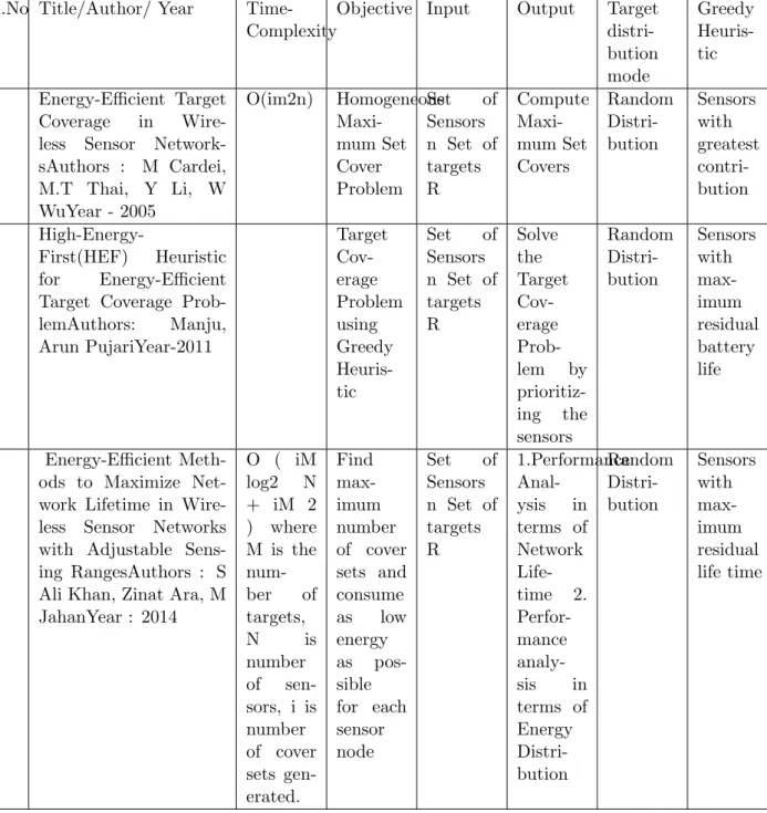
Following are the three examples of sensor deployment using random graph model -Scenario I(fig -2.8) • 40 sensors • 20 targets • 100 m transmission range • 1000×1000 m2 area
.
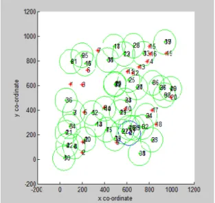
Scenario II:EFFECT OF INCREASE IN TRANSMISSION RANGE(fig -2.9
• 40 sensors
• 20 targets
• 200 m transmisson range
• 1000*1000 m2 area
Figure 2.9: The deployment result when transmission range is increased
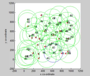
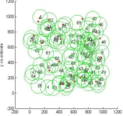
Scenario III:Effect of increase in nodes(fig -2.10)
• 1000*1000 m2 area
Figure 2.10: The deployment result when number of nodes is increased.
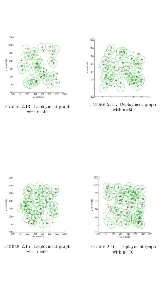
The above implementation was run for many instances and some conclusions were drawn from the results obtained regarding number of sensors sufficient to cover given targets. Following are the results of the above implementation when the number of targets was fixed at 20 and number of sensors were being increased by a count of 10.The sensing range of sensors is 200m .We finally stop at a point when we have sufficient number of sensors so that all the targets lie within the sensing region of one or more than one sensor.
Deployment graph when no. of targets is 20 and no. of sensors is
var-ied.
Figure 2.11: Deployment graph
with n=20
Figure 2.12: Deployment graph
21
Figure 2.13: Deployment graph with n=40
Figure 2.14: Deployment graph with n=50
Figure 2.15: Deployment graph with n=60
Figure 2.16: Deployment graph
Figure 2.17: Deployment graph
with n=80
Figure 2.18: Deployment graph
with n=90
From above results we can draw following
conclusions:-• As the number of sensors are being increased more and more number of targets are being covered.
• When the number of sensors is greater than or equal to 60 very few targets are uncovered.
• In this case when number of sensors is 90 ,all the targets are covered by one or more sensors.
Now let us increase the number of targets from 20 to 25 and find out the number of sensors sufficient to cover all the targets.
23
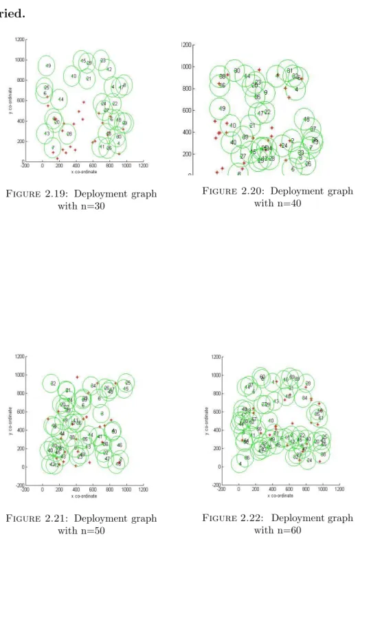
Deployment graph when no. of targets is 25 and no. of sensors is varied.
Figure 2.19: Deployment graph
with n=30
Figure 2.20: Deployment graph
with n=40
Figure 2.21: Deployment graph with n=50
Figure 2.22: Deployment graph
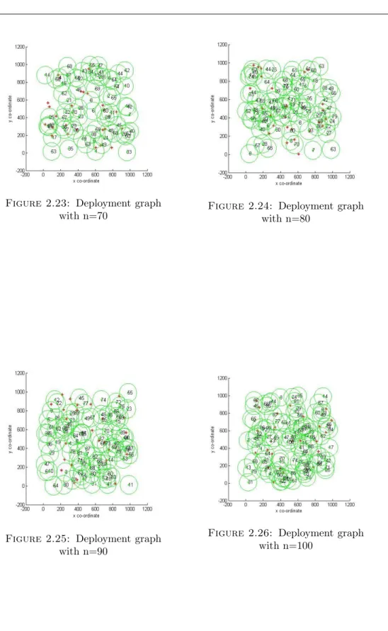
Figure 2.23: Deployment graph
with n=70 Figure 2.24:
Deployment graph with n=80
Figure 2.25: Deployment graph
with n=90
Figure 2.26: Deployment graph
with n=100
From the above graphs following conclusions can be drawn for the case when num-ber of targets is 25
:-25
• When number of sensors is 80 or 90 almost all the targets except 1 or 2 are covered.
• When number of sensors is 100 , all the targets are covered.
Since it is difficult to draw proper conclusions by looking at just 1 or 2 cases, we consider one more case when the number of targets is 30.
Deployment graph when no. of targets is 30 and no. of sensors is varied.
Figure 2.27: Deployment graph
Figure 2.29: Deployment graph with n=50
Figure 2.30: Deployment graph
with n=60
Figure 2.31: Deployment graph with n=70
Figure 2.32: Deployment graph
27
Figure 2.33: Deployment graph
with n=90 Figure 2.34:
Deployment graph with n=100
Figure 2.35: Deployment graph with n=110
Figure 2.36: Deployment graph with n=120
graphs:-• When the number of sensors is greater than or equal to 90 most of the targets are covered.
• When number of sensors is 120 , all the targets are covered.
Observing the above three cases of sensor deployment we note the following points
:-• As the number of targets are increased , more and more number of sensors are needed to supervise the targets.
• Approximately for every five increase in number of targets , 10 or 20 more sensors are required to cover the additional number of targets.
• For an area of 1000×1000m2 4 or 5 times number of targets sensors of range 200m can be placed to cover all the targets.
According to these results we can have a rough idea of approximately how many sensors will be required to cover a set of targets.The result of this section are fur-ther utilized in furfur-ther chapters.We are dealing with two
situations:-• Sensor nodes have fixed sensing and transmission range.
• Sensor nodes have adjustable sensing and transmission ranges.
The first case will be dealt in chapter 3 and second case will be dealt in chapter 4.
Chapter 3
Nodes with Fixed Range
As discussed in the previous chapter, in this thesis we are dealing with the TCP problem in two cases - sensor nodes having fixed range and sensor nodes with variable range.In this chapter, we focus on the first case.That is in this chapter we focus our attention to the target coverage problem in which the objective is to maximize the network lifetime of a wireless sensor network consisting of sensor nodes with fixed range deployed for monitoring a set of targets with known locations.In the next chapter, we will address the same problem with sensor nodes having variable transmission ranges. We here assume a that a number of sensor nodes are deployed randomly in the vicinity of a set of targets.These sensor nodes send the collected information to the sink node, which acts as processing centre. The lifetime of sensor network is defined as the time interval for which every target is covered by at least one sensor node.
3.1
Assumptions
In our experiment, we have assumed the
following:-• A WSN in which a number of small sensor nodes powered by battery are deployed in a target field
• Range of sensor nodes is uniform denoted by r.
• Sensor nodes periodically sense environmental information and send it to sink node where all the processing takes place.
• We denote the set of n sensor nodes by S=s1, s2, s3, , sn.
• We denote the set of m targets by R=r1, r2, , rm.
• Each sensor node can be in three operation modes: sensing, relaying and sleeping.
• We denote the set covers byC =c1, c2, , cp, where each ci for 1<=i <=pis a collection of sensor nodes which collectively can monitor all the targets.
3.2
Problem Statement
Following is our problem statement.This problem statement has been taken from [2]. Let N sensors are there to monitor M targets in WSNs. LetS =s1, s2, , sn and R =r1, r2, .., rn denote the set of senors and set of targets respectively.
The objective is to find a collection of set covers C = c1, c2, , cp with sensing active times t1, t2, , tp in [0, l] for the corresponding set covers such that to maximizet1+t2++tp. , wherelis the lifetime of each sensor at the time of deployment and set covers ci for 1ip are a collection of sensor nodes capable of monitoring all the targets collectively.If a sensor is a part of more than one set cover , the set sum of time interval of those set covers cannot be greater than the lifetime of the sensor.
31
This algorithm has been taken from [2].
This algorithm takes as input the set of sensors ,set of targets,lifetime of a cover set ,sensing range of sensors and lifetime of each sensor and outputs the cover sets such that each and every cover set can monitor all the targets.The total lifetime of the sensor network can then be given by the summation of the lifetime of all cover sets.Here the lifetime of a cover set has been taken as equal to the lifetime of sensors.So the cover sets being formed here are disjoint as each sensor can be a part of only one cover set.
The algorithm starts by checking whether a cover set can be formed or not i.e. whether at least one sensor covers all the targets or not.If not the algorithm halts.Else it finds the most critical target i.e. the target that is covered by least number of sensors.After finding the critical target, from all the sensors that are still active and covers that critical target, a sensor that covers maximum number of still uncovered targets is selected to put in the cover set. All those targets that are covered by the selected sensor are removed from the set of targets.This con-tinues until all the targets are covered, and the cover set is then printed. Again the loop continues to check whether it is possible to frame a new cover set.
Algorithm 3 MSC Algorithm
Require: Set of sensors : SEN SORS , set of targets : R, time each cover set is active : w, sensing range of sensors : r, lif etimeof asensor:t, N :no of sensors
1: i←1 :N
2: for allido
3: Lif e[i] =t
4: end for
5: i←0;
6: while each target is covered by at least1sensor do
7: i:=i+ 1;Ci:= 0;
8: T ARGET S :=R
9: while T ARGET S do
10: find a critical target and a sensor whose lifetime is not zero yet and which covers maximum number of targets while covering critical target.
11: for all targets which are covered by sensor ,remove from TARGETS set.
12: end while
13: Lif e[i] :=Lif e[i]−w
14: end while
33
3.4
Proposed greedy algorithm
The algorithm starts by checking whether a cover set can be formed or not i.e. whether at least one sensor covers all the targets or not.If not the algorithm halts.Else it finds the most critical target i.e. the target that is covered by least number of sensors.After finding the critical target, from all the sensors that are still active and covers the critical target, a score is assigned to each sensor.The sensor getting the highest score is selected and put into the cover set.Then all the targets that are covered by the selected sensor are removed from the list of targets.This continues until all the targets are covered, and the cover set is then printed. Again the loop continues to check whether it is possible to frame a new cover set.
The central point of the algorithm is the score that is assigned to each sensor. The score given to a sensor has been formulated to maximize number of targets covered by the sensor which is uncovered,minimize the number of targets covered by the sensor which is uncovered and maximize the minimum number of sensor which includes the target covered by the sensor.Choosing a sensor which contains maximum number of uncovered targets and minimum number of covered targets from the target cover of the sensor will help us choose an efficient sensor in terms of its utility as a sensor can be fully utilized when all the targets it contains are uncovered.Now one more factor is included in the formula that is we try to choose a sensor having the maximum minimum number of sensors that covers the targets which are included in the target cover of the sensor and has been covered in the present set cover.This will leave the sensor which includes the already covered critical targets(having less number of sensors covering it) in present cover for the next cover.This factor will help us in creating more number of covers by leaving useful sensors(covering critical targets) for next cover if those critical targets have already been covered in the present cover set.
Algorithm 4 MMSC Algorithm
Require: Set of sensors : SEN SORS , set of targets : R, time each cover set is active : w, totaltime:t, N :no of sensors
1: i←1 :N
2: for allido
3: Lif e[i] =t
4: end for
5: i←0;
6: while each target is covered by at least1sensor do
7: i:=i+ 1;Ci:= 0;
8: T ARGET S :=R
9: while T ARGET S do
10: find a critical target
11: j←1 :N
12: for allido
13: score(i)=No. of uncovered targets*minimum of no of sensors covering targets covered by sensor /(No. of covered targets+1)
14: end for
15: select sensor with maximum score.
16: for all targets which are covered by sensor ,remove from TARGETS set.
17: end while
18: Lif e[i] :=Lif e[i]−w
19: end while
3.5
Simulation Results
We evaluate the performance of the MSC and MMSC and Greedy-MSC heuristics which are designed to compute the maximum number of set covers given the set of sensors and set of targets. We simulate a stationary network with randomly dis-persed sensor nodes and target points in a 500m×500m area.We assume the sensing range is uniform for sensors in the network, and that is equal to 200m.Keeping in view the rough conclusions drawn from the previous chapter, the number of sensors starts from 25 as the number of targets starts from 5.In the simulation, following are the tunable parameters:
• The number of sensor nodes denotede by n. We vary the number of sensor nodes between 25 and 75 with a gap of 5 .This will be helpful in studying the effect of node density on the performance.
• the number of targets to be monitored denoted by m. The simulation is carried out with 5 and 10 targets.
From the result, we can conclude that MMSC algorithm performs better than MSC algorithm.
Sensor Nodes with Adjustable
Ranges
In the previous chapter, we worked on the target coverage problem in the case of sensor nodes with transmission range.In this chapter, we explore the target coverage problem of WSNs consisting of sensors with adjustable sensing ranges. Here our objective will be to maximize the lifetime of a power constrained wireless sensor network consisting of sensor nodes with adjustable range deployed for mon-itoring a set of targets with known locations.We will implement a polynomial time algorithm: Adjustable Range Set Cover mentioned in [3]. The algorithm gener-ates a moderate number of cover sets and saves energy as it is possible to choose a smaller sensing range over the larger ones.[3] By utilizing an improved contri-bution formula the selection process of sensor nodes for cover sets gets simplified that ultimately improves the energy efficiency of WSNs.[3]
4.1
Assumtion
• S = s1, s2, , sN represents a collection of N sensor nodes that are deployed randomly to monitor a set of M target nodesT =t1, t2, ., tM.
• Each sensor node siεS, can operate into P sensing ranges R = r1, r2, , rP , where each rk consumes energy ek,1≤k ≤P.
37
• The initial energy of each sensor node is E.
• Linear energy model has been followed for energy consumption ..According to this model ek = c1∗rk , 1 ≤ k ≤ P .c1 is a constant defined as c1 = E/(2∗Σek) ,1≤k ≤P.
• A sensing node sjεS can cover a target tiεT using sensing range rk if the euclidean distance distij is less than or equal to rk , 1 ≤ i ≤ N , 1 ≤ j ≤ M,1≤ k ≤ P Item A cover set Ci is a subset of S that can monitor all the target nodes. Sensor nodes belonging to a particular Ci will be active for a fixed time interval while the remaining nodes are kept in sleep mode and then anotherCj will take the responsibility of monitoring the WSN.
4.2
Problem Statement
Given T = t1, t2, , tM andS = s1, s2, , sN with P adjustable sensing ranges R = r1, r2, , rp , find a collection C of K set covers of size K with minimum possible assignment of sensing ranges such that
-• K is maximized
• all the targets are monitored in each set cover.
• The summation of energy consumed by a sensor appearing in more than one cover set should be less than E.
4.3
Problem scenario
In the previous chapter, we dealt with sensors having fixed range.In this case, we have sensors that can adjust their sensing range.A sensor sensing for a smaller range will consume lesser energy than if the sensor senses for greater range.Choosing a smaller range for sensors(if possible) included in a cover can lead to the reduction
Here we consider four sensors deployed to monitor three targets.Each sensor has two sensing ranges r1 and r2 with r1<r2. Here we assume that sensing region of a sensor is a circular area centered at the sensor having a radius equal to the sensing range.In the figure, the smaller sensing range is denoted by a circle with solid boundary and larger sensing range is denoted by a circle with dotted bound-ary line.The initial energy of sensors is E=2.Energy consumed in sensing smaller range r1 is e1=0.5 and energy consumed in sensing larger range r2 is e2=1. The coverage relationship between sensors, targets, and sensing range is as
follows:-(S1,R1)={T1,T2},(S1,R2)={T1,T2,T3},(S2,R1)={T3},(S2,R2)={T3,T2}, (S3,R1)={T1}
,(S3,R2)={T1,T2} , (S4,R1)={T1,T3} ,(S4,R2)={T1,T3,T2}.This has been de-picted in fig 4.1 and 4.2. .
Figure 4.1: WSN consisting of
3 targets and four sensors with 2 sensing ranges
Figure 4.2: WSN consisting of
3 targets and four sensors with 2 sensing ranges
Now we can have two
solutions:-Solution 1: Here we have three cover sets:- C1={(S1,R2)}, C2={(S4,R1),(S2,R2)}
cover sets can be formed twice.So total lifetime will be 6 unit. Figure 4.3: { C1=(S1,R2) } Figure 4.4: C2={(S4,R1),(S2,R2)} Figure 4.5: C3={(S4,R1) ,(S3,R2)} .
Solution 2: Here the sensing range of all the sensors is fixed to R2. We have two cover sets:- C1={S1} , C2={S2,S4} . Each cover has a lifetime of 1 unit.Each of the above cover sets can be formed twice.So total lifetime will be four units.
Figure 4.6: C1={S1}
Figure 4.7: C2={S2,S4}
In first case, network lifetime is six units when variable ranges are allowed for sensors to attain.In the second case, when the sensing range was fixed, network lifetime attained was four units.Hence, we observe a 50% increment in the life-time. This clearly shows that introducing variable ranges for sensors can lead to the reduction in energy consumption and hence increment in network lifetime.
4.4
ARSC Algorithm
Given the set of sensors,set of targets,set of ranges,and initial energy of sensors this algorithm outputs the set covers formed.For every target, a list of triplets is created.The triplet which can come in the list of a target consists of a sensor which can cover the target, the minimum sensing range with which it can cover the target and the B value for the pair of sensor and range .The B value depends on three factors that are number of targets covered by sensor j within sensing range k, the energy of sensor remained and energy required for a sensor to sense for range k.
41
After ensuring that a cover can be formed i.e. by checking that at least one sensor covers each target , the following procedure is followed until all the targets are covered. The list for every target is sorted according to the value of B. Now from the topmost elements of each list(having maximum B value) the element having maximum B value is selected.The sensor and range mentioned in the element se-lected are chosen for the current cover.All the targets that come within the chosen sensing range of chosen sensor are marked as covered from the list of targets.The energy of the chosen sensor is reduced by the energy that is required for a sensor to cover the chosen range.The value of B is calculated for all the elements of all the lists. This procedure is repeated for until it is not possible to form any more covers. i.e. when any of the targets has no sensor left which can monitor it. .
The time complexity of the above algorithm is O(i∗n∗log(n)∗m+i∗m∗m) , where i is the maximum number of cover sets which can be formed and that will be equal to M ∗E/e1 that is when all the targets are covered by all the sensors
Algorithm 5 ARSC Algorithm
Require: S :set of sensors, T :set of targets, E :initial energy of each sensor, R: ranges of sensors : N : no of sensors, M : no. of targets, P : no of ranges, set of ranges:RAN GES
1: i←1 :M
2: for allido
3: j←1 :N
4: for allj do
5: dist:=distance between SEN SOR[i]AN D T ARGET[j];length[i] = 0;
6: k←1 :P
7: if dist <=RAN GE[k] then
8: Calculate [j,k]and [j,k]
9: [j,k]=No. of targets covered by sensor j within sensing range k.
10: [j,k]=Energy remained of sensor j /energy depleted in covering range k.
11: Length[i]:=length[i]+1; 12: Calculate B[j,k]:=[j,k]*[j,k]; 13: Insert (j,k,B(j,k)) in L(i). 14: end if 15: end for 16: end for 17: q= 0 18: whileallL[i]do 19: i←1 :M 20: for allido
21: do remove exhausted sensors from L[i]
22: end for
23: Sort L[i] in ascending order of B[j,k]
24: q :=q+ 1;Ta:=T;
25: while T a do
26: sensorselected:= 0;rangeselected:= 0;max:= 0;
27: x←1 :M
28: for allxdo
29: if L[i, length[i]].B > max then
30: sensorseleceted:=L[i, length[i]].sensor;
31: rangeselected:=L[i, length[i]].range;
32: end if
33: end for
34: remove all targets covered by sensor selected fromTa
35: end while
36: Push back sensors included in the cover
37: end while
4.5
Simulation results
We evaluate the performance of the ARSC heuristics designed to compute the maximum number of set covers when set of targets and set of nodes are given as input.In simulation ,a stationary network with sensor nodes and target points randomly dispersed in a 100m×100m area is considered. In the experiment in Figure 4, we study the impact of the number of adjustable sensing ranges on the network lifetime.We have considered two cases of 5 targets and 10 targets.We vary the number of sensors between 25 to 75 with a gap of 5.Here P=2 i.e., maximum number of variable ranges is two.The largest sensing range is 60m.We have two cases
-• Adjustable Range Set Cover - sensors have two sensing ranges R1=30m and R2=60m.
• Fixed Range Set Cover - sensors have one sensing range = 60m.
From the results, we can see that ARSC algorithm performs much better that FRSC algorithm.
Genetic Algorithm and Particle
Swarm Optimization
Till now we have discussed greedy techniques for solving the target coverage prob-lem in two cases that is, sensor nodes with fixed range and sensor nodes with variable range.In this chapter, we introduce two natural optimization techniques -Genetic Algorithm and Particle Swarm Optimization.Given a set of current points Greedy algorithms generate new set of points by applying some operators to those points with an aim to move slowly to more optimal places in the search space[4]. It is based on the application of intelligent search of a large and finite search space using statistical methods. [4] .Both algorithms have been implemented, and some conclusions drawn after comparing the results of both algorithms.
5.1
Genetic Algorithm Overview
The genetic algorithm (GA) is an optimization technique based on the rules of natural selection and genetics.This method was found by was developed by John Holland (1975).A GA starts with generating a random population, and then the individuals in the population evolve through natural evolution methods such as mutation,mating, etc. As we proceed through evolution process, we go on re-moving poor individuals from the population and those are replaced by the new
45
individuals derived from better individuals.For measuring the goodness of an in-dividual in the population, we need some mechanism.For that, a cost function is designed such that it would rate good individual high and poor individual low.As such it is an intelligent exploration of a random search space to solve optimization problems.[4]. Although randomized, GAs are by no means totally random because they use historical information of the problem domain to direct the search in a correct direction within the search space.[4].This Genetic Algorithm was developed by Charles Darwin and has been penned down in ”survival of the fittest”[4]. Just as happens in nature GA also utilizes the principle that competition among indi-viduals for scanty resources results in the best indiindi-viduals [4]. Genetic algorithms have efficiently solved many types of optimization problems, and here we apply this technique to solve our optimization problem. Following are the necessary steps of a genetic
algorithm:-1. Define cost function, cost, variables and select GA parameters 2. Initial population is generated
3. Chromosomes are decoded
4. Cost for each chromosome is found 5. Mates are selected.
6. Mating 7. Mutation
8. Convergence Check
9. If maximum iterations reached stop else go to step.3
[4]. First of all the structure of chromosome is decided such that every chro-mosome represents a solution in the search space.Then a cost function is chosen
chromosomes of some fixed size is generated randomly, and all the chromosome in that population is evaluated by the function.In this way, a score is assigned to each chromosome in the population. Based on the fitness value better individu-als are selected as parents to produce offspring via some mating technique. As a result of which highly fit individuals from the population mate with each other so that better characteristics are inherited into the offspring.[5] .Since the size of population is kept fixed and new individuals are being produced ,some of the in-dividuals should be replaced.Less fit inin-dividuals are removed from the population and are replaced by the new solutions.In this way,better individuals are evolved over generations and it is hoped that over successive generations better solutions will evolve.[5]In order to maintain diversity, mutation operator is applied to some individuals.It changes some element of some chromosome to introduce variation.It is used to introduce traits which are not in the original population and keeps the GA from converging prematurely before exploring the entire cost surface. New generations of solutions are produced containing, on average, better genes than the solution in previous generation[5]. Each successive generation produce better ‘partial solutions’ than previous generations[5]. Eventually, once the population has converged and become stabilized i.e. not producing offspring noticeably differ-ent from those in previous generations, the algorithm is said to have converged to a set of solutions for the problem given.[5] Some advantages of genetic algorithm are as
follows:-• It works with both discrete and continuous variables,
• It does not make use of derivatives,
• It has the capability to scale for a large number of variables.,
• It is perfectly suitable for parallel implementation,
• It produces a series of optimum solutions, not just a single solution,
47
5.2
Assumtion
Following are our
assumptions:-• S = s1, s2, , sN represents a collection of N sensor nodes that are deployed randomly to monitor a set of target nodesT =t1, t2, ., tM.
• Range of sensor nodes is uniform.
• A sensing nodesjS can cover a target tiεT if the euclidean distancedistij is less than or equal to r .
• A cover setCi is a subset of S that can monitor all the target nodes. Sensor nodes belonging to a particular Ci will be active for a fixed time interval while the remaining nodes are kept in sleep mode and then another Cj will take the responsibility of monitoring the WSN.
5.3
Problem Statement
Given a collection S of subsets of a finite set T, find the maximum number of disjoint covers for T. Every cover Ci is a subset of S, Ci ⊆ S, such that every element of T belongs to at least one member ofCi, and for any two coversCi and Cj , Ci∩Cj = Φ .
5.4
Implementation Details
After an initial population is initialized to random numbers, the algorithm evolves through the following three operators:
1. selection which selects best individuals according to fitness value as parents for mating;
5.4.1 Chromosome Structure
Each chromosome has size 1×n, where n is the number of sensors. The value of a gene in a chromosome indicates the index number of the group which the sensor joins.The value of a gene is a random number between one and lower bound of optimal cover sets.The Lower bound of the optimal cover set is minimum number of sensors which covers a target.For example ,one chromosome structure that can be formed for below wsn is shown in the figure.Here maximum number of cover sets which can be created is two as 2 sensors cover all the targets.So the value of every gene will be a random number between 1 and 2.So it means sensor 1 is assigned to group 1 ,sensor 2 is assigned to group 2 , sensor 3 is assigned to group 1 ,sensor 4 is assigned to group 2 and sensor 5 is assigned to group 2.
Figure 5.1
5.4.2 Cost Function
Cost function helps to decide better individuals in a population by assigning a fitness value to every chromosome in the population.In our case, the cost function
of a chromosome is defined as the number of cover sets that can be formed by the sensor arrangement of the chromosome.
5.4.3 Selection Operator
Here Roulette wheel weighting method is the parent selection process. The proba-bilities inversely proportional to their cost are assigned to the chromosomes using the following
formula-Pn= (N −n+ 1)/ N
X
n=1
n
Here N is the number of individuals which should be kept unchanged in every interation.A random number between zero and one is generated. Starting from the beginning of the list, the first chromosome with a cumulative probability that is greater than the generated random number is selected for the mating as a parent.Similarly, another individual is selected for mating as second parent.
5.4.4 Crossover Operator
The crossover method used is single point crossover method.Two parents are cho-sen from the population depending upon the fitness value.A crossover point is randomly selected between the first and last gene positions of the parents chromo-somes. First, parent1 passes its gene value to the left of that crossover point to the first child. Then, parent2 passes its binary code to the left of the same crossover point to the second child. Next, the gene values to the right of the crossover point of parent1 goes to the second child and parent2 passes its code to first child. Con-sequently, the offspring contains portions of the binary codes of both parents. For example, 5 is assigned to group 2. The two new offspring created from this mating
5.4.5 Mutation Operator
Random mutations change a some of the gene values of some chromosomes. Mu-tation is the second way a Genetic Algorithm introduces diversity which helps in exploring the cost surface. It can introduce traits not in the original popula-tion and keeps the GA from converging prematurely before exploring the entire cost surface.[5] Its purpose is also to maintain diversity within the population.The best chromosome(having best fitness value) is exempted from the mutation oper-ation.This is known as elitism.So randomlyµ×(Npop−1)×Ngenes, where µis the mutation percent, Npop is the number of chromosomes in a population and ngenes is the number of genes in a chromosome(in our case it will be number of sensors) , genes are selected and their values changed to some other value. For example,
Figure 5.3
5.5
The Genetic Algorithm
This algorithm takes as input maximum number of iterations,population size,mutation rate,selection ratio,number of parameters and an array containing the number of sensors which covers each targets and returns as output the number of cover sets formed. The algorithm starts by calculating keep which is the number of individ-uals which have to be retained for next iteration and limit which is the maximum number of cover sets which can be formed by the given configuration of sensors and targets.The minimum number of cover sets which can be created will be equal to the minimum number of sensors which covers a target.A random population is generated.This random population is a 2-D array of dimension popsize x N ,where
51
each entry is a random number between 1 and limit.Every individual in the popu-lation is evaluated using cost function and are sorted in descending order so that all the good individuals is at the top of the pop array. .
The following procedure is repeated for maximum iteration given.The population that has to be removed is calculated in M, and those individuals are assigned a probability.A rank is assigned to M individuals based on the cost function(topmost element 1 and so on).The probability assigned is the cumulative sum of rank di-vided by the sum of the rank of M individuals.For these M individuals, two random values are calculated.These two random values help in choosing mother and father for the individual.The first element whose probability is greater than the random numbers, are selected as mother and father respectively for M individuals and stored in father and mother respectively.Those M individuals are replaced by mat-ing(as explained previously) of father and mother.After that, the number of genes to be mutated is calculated, and then those many random genes are selected, and their values are changed.New individuals are evaluated and again sorted.
Finally, the topmost cost function that contains the number of cover sets formed by the best individual till now, is returned.
Algorithm 6 M SCGAAlgorithm
Require: max number of iterations : maxit, size of population : popsize, mutation rate:mutrate, selection ratio :selection, no of parameters : N , npar no of sensors by which each target is covered:target cover no
1: keep←selection∗popsize
2: limit← minimum in target cover no
3: i←1 :popsize
4: for allido
5: j←1 :N
6: for allj do
7: pop(i, j) =random number between1 and limit
8: end for
9: end for
10: Sort population and cost in descending order.
11: iteration←1 :maxit 12: for alliterationdo
13: M ←(popsize−keep)/2
14: i←1 :keep
15: for allido
16: probability(i)←2∗i/(keep∗(keep+ 1))
17: end for
18: i←1 :M
19: for allido
20: pick1(i) =random number between0 and1
21: pick2(i) =random number between0 and1
22: end for
23: i←1 :M
24: for allido
25: j←1 :keep+ 1
26: for alljdo
27: if pick1(i)<=probability(j)andpick1(i)> probability(j−1)then
28: mother(i) =j−1
29: end if
30: if pick2(i)<=probability(j)andpick2(i)> probability(j−1)then
31: f ather(i) =j−1 32: end if 33: end for 34: end for 35: i←1 : 2 :keep 36: for allido 37: P t:=rand(1, M)∗n
38: P op(keep+i,:) = [pop(mother,1 :pt)pop(f ather, pt+ 1 :n)]
39: P op(keep+i+ 1,:) = [pop(f ather,1 :pt)pop(mother, pt+ 1 :n)]
40: end for
41: N o←(popsize−1)∗n∗mutrate
42: Row←rand(1, no)∗(popsize−1) + 1
43: Col←rand(1, no)∗n
44: j←1 :N o
45: for allj do
46: P op(row(j), col(j))←rand(1,1)∗(ub−1) + 1
47: end for
48: cost←costfunc(pop) .
Sort cost and pop in descending order
49: end for.
5.6
Simulation Results
We evaluate the performance of the Genetic algorithm designed to maximize the number of set covers. We have simulated a stationary network with sensor nodes and target points randomly dispersed in a 500m×500m area. In the experiment in Figure 5.4, we compare the performance of three algorithms
1. MSC - The greedy algorithm mentioned in chapter three.
2. ,M SCRd- The random algorithm that randomly assigns sensors to set covers. 3. M SCGA- The genetic algorithm
Figure 5.4
Figure 5.5
Figure 5.6
Figure 5.7
From the figure, we can conclude that the genetic algorithm performs better than greedy algorithm and random algorithm in most of the cases.
5.7
Particle Swarm Optimization
Particle swarm optimization (PSO) is a population based stochastic optimization technique developed in 1995 by Dr. Eberhart and Dr. Kennedy .It is encouraged by social behavior of bird flocking or fish schooling.[6] PSO is very much similar to evolutionary computation techniques such as Genetic Algorithms (GA). Just like genetic algorithm initially system is initialized with a population of random solutions and then keeps on searching for optima by updating generations. How-ever, unlike GA, PSO has no evolution operators such as crossover and mutation. In PSO, the potential solutions, called particles, move through the problem space by following the current optimum particles[6]. Compared to GA, the advantages of PSO are that PSO is easy to implement, and there are (as compared to former) few parameters to adjust. PSO has been successfully applied in many areas: It-erated Prisoner’s Dilemma, artificial neural network training, traveling salesman
55
problem, and other areas where GA can be used. We will use PSO to solve the TCP problem in the case of sensors with fixed range.
5.8
Overview of Particle Swarm Optimization Algorithm
As stated before, PSO follows the behavior of a group of bird searching for food. Let us consider the following scenario: a group of birds is randomly searching for food in some area. There is just one piece of food in the area being explored. None of the bird knows where the food is. But they know how much near to the food are they in each iteration. So in this situation the best strategy to find the food is to follow the bird that is nearest to the food[6]. PSO utilizes the same technique to solve the optimization problems. In PSO, each single solution is a ”bird” searching for food in the search space. [6]We call it ”particle.” All of the particles have fitness values that are evaluated by the fitness function(depends on the problem) to be optimized, and have velocities that direct the flying of the particles[6]. The particles fly through the problem space by following the current optimum particles. The PSO is a population-based search algorithm based on the social behavior of a group of birds, bees or a school of fishes.[6] Initially, a swarm is created and initialized randomly. Each individual within the swarm is represented by a vector in the multidimensional search space.In our case, the number of dimensions will be equal to the number of sensors.A velocity vector is also initialized randomly which will direct the movement of these particles through the search space. The PSO algorithm in every iteration updates the velocity as well as position of each particle in the population. Each particle updates its velocity based on three factors - current velocity , best position it has explored till now and the global best position examined by the swarm[6].The position of a particle is updated according to the updated velocity of the particle. The PSO process then is carried out for a fixed number of times or until a minimum error is achieved. Let bestp be the array having the best position achieved by every particle so far