Performance Analysis of Fixed-Random Weights in Artificial Neural Networks

(1)

Rochester Institute of Technology Rochester Institute of Technology

RIT Scholar Works

Theses

6-2019

Performance Analysis of Fixed-Random Weights in Artificial

Neural Networks

Humza Syed

[email protected]

Follow this and additional works at: https://scholarworks.rit.edu/theses

Recommended Citation Recommended Citation

Syed, Humza, "Performance Analysis of Fixed-Random Weights in Artificial Neural Networks" (2019). Thesis. Rochester Institute of Technology. Accessed from

This Thesis is brought to you for free and open access by RIT Scholar Works. It has been accepted for inclusion in Theses by an authorized administrator of RIT Scholar Works. For more information, please contact

(2)

Performance Analysis of Fixed-Random Weights

in Artificial Neural Networks

(3)

Performance Analysis of Fixed-Random Weights

in Artificial Neural Networks

Humza Syed June 2019

A Thesis Submitted in Partial Fulfillment

of the Requirements for the Degree of Master of Science

in

Computer Engineering

(4)

Performance Analysis of Fixed-Random Weights

in Artificial Neural Networks

Humza Syed

Committee Approval:

Dr. Dhireesha Kudithipudi Advisor Date

Professor, RIT, Department of Computer Engineering

Dr. Cory Merkel Date

Assistant Professor, RIT, Department of Computer Engineering

Dr. Raymond Ptucha Date

(5)

Acknowledgments

I would like to acknowledge my adviser, Dr. Dhireesha Kudithipudi, and the members of the Neuromorphic AI Lab at the Rochester Institute of Technology for helping make this work possible. I would also like to acknowledge Dr. Panos Markopoulos for assistance in understanding tensor decompositions and the Air Force Research Labs for helping to fund part of this work. Lastly, I would like to acknowledge my friends and family who have supported me throughout my college career.

(6)

I would like to dedicate this work to my family who have continuously supported me throughout my life. My father would have been proud to see how far I’ve come and

(7)

Abstract

Deep neural networks train millions of parameters to achieve state-of-the-art per-formance on a wide foray of applications. However, finding a global minimum with gradient descent approaches leads to lengthy training times coupled with high compu-tational resource requirements. To alleviate these concerns, the idea of fixed-random weights in deep neural networks is explored. More critically the goal is to maintain performance akin to fully trained models.

Metrics such as floating point operations per second and memory size are compared and contrasted for fixed-random and fully trained models. Additional analysis on downsized models that mimic the number of trained parameters of the fixed-random models, shows that fixed-random weights enable slightly higher performance. In a fixed-random convolutional model, ResNet achieves ∼57% image classification accu-racy on CIFAR-10. In contrast, a DenseNet architecture, with only fixed-random fil-ters in the convolutional layers, achieves∼88% accuracy for the same task. DenseNet’s fully trained model achieves ∼96% accuracy, which highlights the importance of ar-chitectural choice for a high performing model.

To further understand the role of architectures, random projection networks trained using a least squares approximation learning rule are studied. In these networks, deep random projection layers and skipped connections are exploited as they are shown to boost the overall network performance. In several of the image classification experi-ments conducted, additional layers and skipped connectivity consistently outperform a baseline random projection network by 1% to 3%. To reduce the complexity of the models in general, a tensor decomposition technique, known as the Tensor-Train de-composition, is leveraged. The compression of the fully-connected hidden layer leads to a minimum ∼40x decrease in memory size at a slight cost in resource utilization. This research study helps to gain a better understanding of how random filters and weights can be utilized to obtain lighter models.

(8)

Contents

Signature Sheet i Acknowledgments ii Dedication iii Abstract iv Table of Contents v

List of Figures vii

List of Tables xv

Acronyms xvii

1 Introduction 1

1.1 Research Motivation . . . 1

1.2 Research Objectives . . . 2

2 Background & Related Work 6 2.1 The Perceptron and Multi-Layer Perceptrons . . . 6

2.2 Convolutional Neural Networks . . . 10

2.2.1 AlexNet . . . 11

2.2.2 VGG . . . 13

2.2.3 ResNet . . . 13

2.2.4 DenseNet . . . 14

2.3 Random Weights in ANNs . . . 15

2.3.1 The Importance of Architecture Design . . . 16

2.3.2 Random Weights in DNNs Achieving Comparable Performance 16 2.4 Random Projection Networks . . . 23

2.4.1 ELM . . . 23

2.4.2 Random Vector Functional Link Network . . . 25

2.5 Tensor Decomposition . . . 26

(9)

List of Figures

2.1 Illustration of a Perceptron taking the weighted sum of its inputs and an additional bias term. . . 7 2.2 Illustration of an MLP. In this architecture each progressive layer takes

the weighted sum of its inputs. . . 8 2.3 The LeNet-5 shallow CNN architecture consisting of convolutional,

pooling, and FC layers [1]. . . 12 2.4 The AlexNet CNN architecture consisting of multiple convolutional,

pooling, and FC layers illustrating the impact of deep neural networks [2]. . . 12 2.5 A ResNet residual block consisting of the use of skipped additive

con-nectivity to alleviate the vanishing and exploding gradient problems [3]. . . 14 2.6 A DenseNet dense block consisting of the use of skipped concatenating

connectivity to increase the number of features extracting in each layer [4]. . . 15 2.7 Reconstructions of 3 images when utilizing a fully random VGG net

and a fully trained VGG net [5]. The visualization from the pool5 layer exhibits certain features learned in the trained net that inhibits reconstruction. . . 17 2.8 Generated textures from several images when utilizing a fully random

VGG net and a fully trained VGG net [5]. In this figure each row corresponds to a convolutional layer in the random VGG net while a comparison is made between the 4th convolutional layer of both the trained and random nets. . . 18 2.9 Neural style transfer of images when utilizing a fully random VGG net

and a fully trained VGG net [5]. The first row depicts the original image, while the second and third rows show the random VGG net and trained VGG net’s content images with the applied style transfer. Note: The reference [13] in this image refers to [6]’s paper. . . 19

(11)

LIST OF FIGURES

2.10 Experiments utilizing a percentage and a k amount of trained weights in deep Convolutional Neural Network (CNN) architectures. The white area indicates the percentage of weights trained, while the gray area indicates training on only k number of filters per convolutional layer. The blue line indicates the rest of the weights in the layer were left untrained, while the green line indicates the rest of the weights in the layer were zeroed out [7]. . . 20 2.11 The WRN and DenseNet networks compared on both the CIFAR-10

(left) and CIFAR-100 (right) datasets at various training fractions per convolutional layer. Green and blue solid lines indicate networks with a fraction of trained weights and the rest left random. Green and blue dashed lines indicate the performance of the WRN and DenseNet networks with trained weights. Note: when frac = 1.0, this is actually when only a single filter is trained per convolutional layer [7]. . . 22 2.12 Illustration of tensors in varying orders, or dimensions. . . 26 2.13 Illustration of a tensor decomposition in which an input T is

approxi-mated by the summation of rank-one tensors. These rank-one tensors are calculated from the outer product of 1st order tensorsa, b, and c. 28 2.14 Illustration of the Tucker decomposition in which an input T is

ap-proximated into a compressed core G. This compressed core is then multiplied by the matrices representing rank-one tensors;A,B, andC. 29 2.15 Illustration of a 5th order tensor decomposition into respective cores

of the Tensor-Train (TT) format. . . 31

3.1 The CIFAR-10 dataset containing various classes ranging from air-planes to trucks [8]. . . 35 3.2 The SVHN dataset containing digits 0 through 9 in a similar manner

to MNIST, but in natural scenery [9]. . . 35 3.3 The UCM dataset containing aerial imagery of 21 classes [10, 11]. . . 36 3.4 The MSTAR dataset containing 10 unique vehicle classes [12]. . . 37 3.5 The small NORB dataset containing 5 classes ranging from four-legged

animals to cars [13]. . . 37 3.6 The FMNIST dataset containing 10 classes of fashion items ranging

(12)

LIST OF FIGURES

3.7 Diagram depicting the operations required for SGD. (a) illustrates the forward pass as well as the error calculation and gradient calculation for the backward pass. (b) illustrates the weight update as well as calculations for regularization and momentum [15]. . . 41 3.8 Illustration of the CELM architecture which makes use of an initial

convolution layer as a feature extractor and then 2 FC layers. Skipped connections are utilized to observe their effectiveness in the possibility of increasing performance. . . 43 3.9 Illustration of the CRVFL-FC architecture. A convolutional layer is

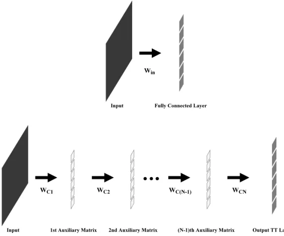
used to extract features that are sent to a pooling layer to reduce the spatial size of the feature maps. A normalization layer is used to decrease covariance shift and then the output is fed to the last 2 Fully Connected (FC) layers. A skipped connection is used from the input to the first FC layer as this was used in the original architecture. . . . 44 3.10 Illustration of an FC layer and its representation in a TT-FC layer

format. The initial layer’s inputs are decomposed into several TT cores that act as unfolded auxiliary matrices to the output. . . 45

4.1 Plot of each ResNet-20 configuration on the Canadian Institute for Advanced Research (CIFAR)-10 dataset averaged over 10 runs with a confidence interval of 99%. Fixed-random refers to the case of trained and fixed-random filters and downsized refers to the case of fewer filter models. The case of Linear refers to the increase of trained weights with each convolutional layer in the network. It’s noted that models with trained and fixed-random filters outperform the downsized versions of the models across all cases. This difference is more noticeable at smaller fractional amounts of trained filters. This is due to the fixed-random filters enabling for a greater feature space to be extracted from in comparison to the downsized models. . . 49

(13)

LIST OF FIGURES

4.2 Statistics plot of each ResNet-20 configuration on the CIFAR-10 dataset averaged over 10 runs with a confidence interval of 99%. The config-urations consist of fixed-random filters in the convolutional layer and downsized models with fewer filters in the convolutional layer. It can be seen that the downsized filter models utilize fewer Giga-FLOPs (GFLOPs) in comparison to the fixed-random and fully trained mod-els. This is because the fixed-random filter models need to backprop-agate the entire network back due to their mix of trained and random filters. In contrast, downsized models demand fewer resources because less filters are utilized in these models as well as fewer operations on the last FC layer. . . 51 4.3 Image of a frog from CIFAR-10. . . 52 4.4 Image of an automobile from CIFAR-10. . . 52 4.5 Activated outputs of each convolutional layer in ResNet-20 on the input

image of a frog from CIFAR-10. Features can be seen to be more distinguishable in the early layers as opposed to the latter layers of the architecture. . . 53 4.6 Activated outputs of each convolutional layer in ResNet-20 on the input

image of an automobile from CIFAR-10. Similarly to the frog, features can be seen to be more distinguishable in the early layers as opposed to the latter layers of the architecture. . . 53 4.7 Plot of each ResNet-20 configuration on the Street View House

Num-bers (SVHN) dataset averaged over 10 runs with a confidence interval of 99%. Fixed-random refers to the case of trained and fixed-random filters and downsized refers to the case of fewer filter models. The case of Linear refers to the increase of trained weights with each convolu-tional layer in the network. Unlike the results from CIFAR-10, random projection shows a surprisingly high performance, while the other mod-els show more comparable performances to one another. This is most likely due to the higher number of training samples and possibly more simple imagery in comparison to CIFAR-10. . . 55

(14)

LIST OF FIGURES

4.8 Statistics plot of each ResNet-20 configuration on the SVHN dataset averaged over 10 runs with a confidence interval of 99%. The config-urations consist of fixed-random filters in the convolutional layer and downsized models with fewer filters in the convolutional layer. The downsized models utilize fewer GFLOPs as less operations are occur-ring in these networks. Additionally, the downsized models require fewer operations in their forward passes leading to a greater decrease in the number of operations and an additional decrease in memory size as fewer parameters are available in these models. The fixed-random models utilize a similar amount of GFLOPs to the fully trained models due to backpropagation occurring across all layers. . . 57 4.9 Plot of each DenseNet100-BC configuration on the CIFAR-10 dataset

averaged over 5 runs with a confidence interval of 99%. Fixed-random refers to the case of trained and fixed-random filters and downsized refers to the case of fewer filter models. The case of Linear refers to the increase of trained weights with each convolutional layer in the network. The performance of random projection shows surprisingly that DenseNet’s concatenating skipped connectivity can be beneficial with random weights as features are extracted and trained on at the last FC layer of the architecture. . . 58 4.10 Statistics plot of each DenseNet100-BC configuration on the CIFAR-10

dataset averaged over 5 runs with a confidence interval of 99%. The configurations consist of fixed-random filters in the convolutional layer and downsized models with fewer filters in the convolutional layer. Similarly to the previous statistic plots, the downsized models show a decrease in GFLOPs and memory size over the fixed-random models. In addition to this, the fixed-random weights for random projection is shown to actually have approximately 12% of the weights trained. This is due to the concatenation skipped connectivity leading to more features trained on the output layer. . . 61 4.11 Activated outputs of every 5 convolutional layers of DenseNet100-BC

on the input image of a frog from CIFAR-10. Features can be seen to be more distinguishable in the early layers as opposed to the latter layers of the architecture. . . 62

(15)

LIST OF FIGURES

4.12 Activated outputs of every 5 convolutional layers of DenseNet100-BC on the input image of an automobile from CIFAR-10. Similarly to the frog, features can be seen to be more distinguishable in the early layers as opposed to the latter layers of the architecture. . . 63 4.13 Plot of each DenseNet100-BC configuration on the SVHN dataset

av-eraged over 5 runs with a confidence interval of 99%. Fixed-random refers to the case of trained and fixed-random filters and downsized refers to the case of fewer filter models. The case of Linear refers to the increase of trained weights with each convolutional layer in the network. In contrast to the results from CIFAR-10, random projec-tion shows high performance comparable to that of the other models. This may be due to the additional samples available to train on for the few trained layers of the network. In addition to this, the other ar-chitectures illustrate near comparable performance to the fully trained model. . . 64 4.14 Statistics plot of each DenseNet100-BC configuration on the SVHN

dataset averaged over 5 runs with a confidence interval of 99%. The configurations consist of fixed-random filters in the convolutional layer and downsized models with fewer filters in the convolutional layer. Similarly to the previous statistic plots, the downsized models show a decrease in GFLOPs and memory size over the fixed-random models. The random projection model with only fixed-random convolutional layers is shown to have approximately 12% of the weights trained due to concatenated features trained on the output layer. . . 66 4.15 Plot of each ResNet-50 transfer learning configuration on the SVHN

dataset averaged over 10 runs with a confidence interval of 99%. Fixed refers to the case of trained and fixed filters, from the pretrained model, and Linear refers to the increase of trained weights with each convo-lutional layer in the network. Fine-tuning the entire network shows increased performance over partial fine-tuning, however, near compa-rable accuracies can be achieved with partial fine-tuning and fewer resources are utilized as fewer memory writes occur. Additionally, the results show that performance over that of Scott et al.’s work [16] can be achieved with the partial fixed networks. . . 67

(16)

LIST OF FIGURES

4.16 Performance of the random projection architectures on the Moving and Stationary Target Acquisition and Recognition (MSTAR) dataset. The CELM network with skipped connectivity to both the FC layers shows the highest test accuracy as more features are available on the output

to train on. . . 70

4.17 Statistics of the random projection architectures on the MSTAR dataset. The architectures utilizing additional layers require more GFLOPs and additional memory to store all of their parameters. It’s important to note that the Tensor-Train Extreme Learning Machine (TT-ELM) and TT-Random Vector Functional Link Neural Network (RVFL) are able to achieve a smaller model with the cost of more GFLOPs due to the additional operations occurring in the layer. . . 71

4.18 Performance of the random projection architectures on the small-NYU Object Recognition Benchmark (NORB) dataset. Similarly to the MSTAR dataset, the Convolutional ELM (CELM) with skipped con-nectivity to both FC layers achieves the highest performance as addi-tional features are trained in this layer. . . 72

4.19 Statistics of the random projection architectures on the small-NORB dataset. The architectures utilizing additional layers require more GFLOPs and additional memory to store all of their parameters. The TT networks achieve a smaller model at the cost of additional GFLOPs due to the additional operations occurring in the layer. . . 73

4.20 Performance of the random projection architectures on the Fashion-MNIST (FFashion-MNIST) dataset. As with the other datasets, the CELM with skipped connectivity to both FC layers achieves the highest per-formance. However, there is less of a distinguishable gap in this more complex dataset. . . 74

4.21 Statistics of the random projection architectures on the FMNIST dataset. The architectures utilizing additional layers require more GFLOPs and additional memory to store all of their parameters. The TT networks achieve a smaller model at the cost of additional GFLOPs due to the additional operations occurring in the layer. . . 75

5.1 Image of an airplane from CIFAR-10. . . 87

5.2 Image of a dog from CIFAR-10. . . 87

(17)

LIST OF FIGURES

5.4 Activated outputs of each convolutional layer in ResNet-20 on the input image of an airplane from CIFAR-10. Features can be seen to be more distinguishable in the early layers as opposed to the latter layers of the architecture. . . 87 5.5 Activated outputs of each convolutional layer in ResNet-20 on the input

image of a dog from CIFAR-10. Similarly to the frog, features can be seen to be more distinguishable in the early layers as opposed to the latter layers of the architecture. . . 88 5.6 Activated outputs of each convolutional layer in ResNet-20 on the input

image of a truck from CIFAR-10. Similarly to the frog, features can be seen to be more distinguishable in the early layers as opposed to the latter layers of the architecture. . . 88 5.7 Activated outputs of every 5 convolutional layers of DenseNet100-BC

on the input image of an airplane from CIFAR-10. Similarly to the other activated images, features can be seen to be more distinguishable in the early layers as opposed to the latter layers of the architecture. 89 5.8 Activated outputs of every 5 convolutional layers of DenseNet100-BC

on the input image of a dog from CIFAR-10. Similarly to the other activated images, features can be seen to be more distinguishable in the early layers as opposed to the latter layers of the architecture. . 90 5.9 Activated outputs of every 5 convolutional layers of DenseNet100-BC

on the input image of a truck from CIFAR-10. Similarly to the other activated images, features can be seen to be more distinguishable in the early layers as opposed to the latter layers of the architecture. . 91

(18)

List of Tables

2.1 Performance achieved when learning only a fraction of filters for the CIFAR-10 dataset for training epochs of 200 on WRN and 300 on densenets. Eff. Params indicates the number of trained parameters, while * indicates the performance when the parameters for random weights were zeroed out [7]. . . 21 2.2 Performance on the Tiny-ImageNet dataset using the WRN model with

various percentages of trained weights [7]. . . 22

4.1 Performance on the CIFAR-10 dataset using the ResNet-20 architec-ture. A dividing line is used to separate networks with trained and fixed-random filters and downsized networks with fewer filters. The network is averaged over 10 runs and a confidence interval of 99% is used. From the results, the fixed-random networks are able to achieve more comparable accuracies to the fully trained model as opposed to the downsized network cases. . . 50 4.2 Performance on the SVHN dataset using the ResNet-20 architecture.

A dividing line is used to separate networks with trained and fixed-random filters and downsized networks with fewer filters. The network is averaged over 10 runs and a confidence interval of 99% is used. The results illustrate clearly how the fixed-random models outperform the downsized models even if marginally. Additionally, the random projection network shows a surprisingly high accuracy. This may be attributed to additional samples and possibly more simple imagery. . 56 4.3 Performance on the CIFAR-10 dataset using the DenseNet100-BC

ar-chitecture. A dividing line is used to separate networks with trained and fixed-random filters and downsized networks with fewer filters. The network is averaged over 5 runs and a confidence interval of 99% is used. From the results, the fixed-random networks are able to achieve more comparable accuracies to the fully trained model as opposed to the zeroed out network cases. In addition to this, the random projec-tion network with a 0 trained fracprojec-tional amount is able to achieve over 88% accuracy. . . 59

(19)

LIST OF TABLES

4.4 Performance on the SVHN dataset using the DenseNet100-BC archi-tecture. A dividing line is used to separate networks with trained and fixed-random filters and downsized networks with fewer filters. The network is averaged over 5 runs and a confidence interval of 99% is used. The results show surprisingly that both fixed-random and down-sized models lead to performance extremely similar to the fully trained model. The random projection case even shows performance akin to the fully trained model. This may be attributed to a greater num-ber of samples available as well as simpler imagery when compared to CIFAR-10. . . 65 4.5 Performance on the CIFAR-10 dataset after training each deep CNN

for additional epochs up until 500 total trained epochs. . . 65 4.6 Performance on the UCM dataset by transfer learning the ResNet-50

architecture. The network is averaged over 10 runs and a confidence interval of 99% is used. A dividing line is used to separate the fixed networks fine-tuned in this work compared to that of Scott et al. [16]. Near comparable accuracies can be achieved with partial fine-tuning in comparison to entire fine-tuning of the network. In all cases, except for only training the FC layer of the network, the accuracy is shown to surpass that of the work of Scott et al. [16]. . . 68

(20)

Acronyms

ANN

Artificial Neural Network

ANNs

Artificial Neural Networks

CELM

Convolutional ELM

CIFAR

Canadian Institute for Advanced Research

CNN

Convolutional Neural Network

CNNs

Convolutional Neural Networks

CP

canonical polyadic

CPUs

Central Processing Units

CRVFL

Convolutional Random Vector Functional Link Neural Network

(21)

Acronyms

DNNs

Deep Neural Networks

ELM

Extreme Learning Machine

ESN

Echo State Network

FC

Fully Connected

FLOPs

Floating Point Operations per Second

FMNIST

Fashion-MNIST

GFLOPs

Giga-FLOPs

GPUs

Graphics Processing Units

LSM

Liquid State Machine

MLP

(22)

Acronyms

MNIST

Mixed National Institute of Standards and Technology

MPP

Moore-Penrose Pseudoinverse

MSTAR

Moving and Stationary Target Acquisition and Recognition

NORB

NYU Object Recognition Benchmark

PCA

Principle Component Analysis

ReLU

Rectified Linear Unit

RVFL

Random Vector Functional Link Neural Network

SGD

Stochastic Gradient Descent

SVHN

Street View House Numbers

TT

(23)

Acronyms

TT-ELM

Tensor-Train Extreme Learning Machine

UAVs

Unmanned Aerial Vehicles

UCM

UC Merced Land Use

VGG

Visual Geometry Group

WRN

(24)

Chapter 1

Introduction

Deep Neural Networks (DNNs) are achieving state-of-the-art performance in several application domains such as image classification [17], target detection [18], and fore-casting tasks [19]. The backpropagation algorithm [20] in these networks can train the weighted parameters to learn important features from their inputs. This enables the network to generalize to new data and classify the data to their respective classes.

1.1

Research Motivation

Unfortunately, the iterative update of these weighted parameters is a computation-ally intensive process with long training times. For example, convolutional neural networks (CNNs) (eg: AlexNet [2] and ResNet [3]), require lengthy training times for complex tasks, such as ImageNet [21]. More recent studies show that training AlexNet on ImageNet for 100 epochs and a batch size of 512 on the powerful DGX-1 station requires 6 hours and 10 minutes [22]. Training ResNet-50 on ImageNet for 90 epochs and a batch size of 256 on a DGX-1 station requires 21 hours [22]. Al-ternatively, with enough computational resources, such as 3,456 Tesla V100 GPUs, ResNet-50 was trained in 2 minutes [23].

Such long training times and massive demand on resources are impractical for a growing subset of applications, such as lifelong learning systems [24] and edge appli-cations [25, 26]. For example, in [27], the authors focus on utilizing Convolutional

(25)

CHAPTER 1. INTRODUCTION

Neural Networks (CNNs) for on-device object detection in Unmanned Aerial Vehicles (UAVs). They observe that conventional DNNs incur high computational costs to process frames of a video on-device. Additionally, in many UAVs, Central Processing Units (CPUs) are used over Graphics Processing Units (GPUs) due to power con-cerns. This work showcases lightweight networks designed for resource constrained applications. A critical design constraint is to design algorithms that can be trained on-device, in real-time, to adapt to dynamic environments. Another example is learn-ing from few samples through methodologies such as meta-learnlearn-ing [28]. In [28], the authors illustrate how specialized training techniques can enable for networks to train on few samples with minimal gradient calculations. This leads to a network that can train quickly for new tasks. This type of training methodology is ideal for continual lifelong learning systems that require learning new tasks quickly in a computationally efficient fashion. In contrast to faster training models, faster inference models with low latency features are available to accelerate the post-deployment phase of DNNs [29, 30]. However, the training time bottleneck for large and small datasets, is still an active research problem [31, 32]. With the evolving need to move training to the edge, it is critical to study compute-lite architectures with fast training times.

1.2

Research Objectives

The central objective of this research is to study how fixed-random weights can poten-tially reduce resources and training time in Artificial Neural Networks (ANNs) and deep CNNs while retaining high performance. In this context, fixed-random weights refer to weights that are initialized to a random value and then left untrained, or fixed, throughout the network’s training process. The utilization of fixed-random weights is one methodology for decreasing training time and resource utilization. Other method-ologies include the usage of compression [33] or pruning [34] to decrease the number of parameters in a pre-trained network or while training the network. This can lead

(26)

CHAPTER 1. INTRODUCTION

to a decrease in the number of Floating Point Operations per Second (FLOPs) for the forward pass of the network, which can be beneficial for inference. However, these techniques do not address the amount of time needed to train these networks as addi-tional computations can occur from the compression or pruning overhead [35, 36, 37]. Alternatively, the use of fixed-random weights can potentially allow for reduced train-ing time while retaintrain-ing the network’s large parameter space. Maintaintrain-ing the large parameter space can be beneficial as the input’s initial dimensionality can be ex-tracted into a larger dimensionality allowing for separability between the data [38]. This can enable the network to optimize its trained weights while leveraging the features extracted from the random weights. To evaluate the use of fixed-random weights, various methodologies are explored in this work, such as setting entire lay-ers of networks to fixed-random weights, setting portions of laylay-ers to fixed-random weights, and setting the first layer of a network to fully random, or 100% random, and then slowly decreasing the percentage of random weights in layers further down throughout the network’s architecture.

In addition to the above methodologies, the second objective of this work is to ex-tend the architecture of random projection networks trained using the Moore-Penrose Pseudoinverse (MPP) [39] to approximate the least squares solution [40, 41, 42, 43, 44, 45]. These networks are shown to train in orders of magnitude faster than stochas-tic gradient descent approaches. In [43] and [44], a CNN is first trained end to end with a softmax classification layer and then transfer learned as a feature extractor for a random projection network that is used in place of the fully-connected layers from the original CNN. This method enabled their models to achieve high performance on digestive organ classification for wireless capsule endoscopy and traffic sign recogni-tion. Unfortunately, these works don’t highlight the memory requirements for the transfer learned models. In [45], the authors train a random projection network with convolution and pooling layers. The network utilized random weights in all layers and

(27)

CHAPTER 1. INTRODUCTION

only trained on the output layer. The authors showed that high performance could be achieved on handwritten digit recognition, but didn’t address the memory required with the addition of each additional layer. Additionally, few works explore the use of skipped connectivity in random projection literature [46, 47, 48]. The use of skipped connectivity was shown to increase performance in these works but this connection was limited to skipped connectivity from the input to the output layer and did not further explore the use of greater connectivity. Increased skipped connectivity may be beneficial to explore as these connections have been shown to boost the performance of many DNNs today [3, 4]. To address these concerns, random projection networks are extended further with additional layers, containing fixed-random weights, as well as concatenating skipped connectivity, similar to that of DenseNet [4]. The use of additional random projection layers are shown to lead to transformations in the data that are beneficial for the trained portion of these networks. Likewise, the use of skipped concatenating connectivity allows for earlier layer features to be utilized in the training process to obtain optimal weights.

The third objective is to use a tensor decomposition technique to support com-pressed layers in an Extreme Learning Machine (ELM) and thereby reduce the model size. Tensor decomposition allows for tensors, or multi-dimensional arrays, to be transformed into their respective low-rank model enabling for an approximation of the original model. This can potentially lead to a decrease in parameters and lead to savings in resource utilization. This idea is utilized in a random projection net-work to decrease the demand on memory and to assess if a high performance model can be achieved with little to no performance drop as compared to its uncompressed counterpart.

To summarize, the main objectives of this work are the following:

1. Empirically evaluate the performance of networks utilizing fixed-random weights and assess the benefits of using this technique in comparison to smaller

(28)

equiv-CHAPTER 1. INTRODUCTION

alent networks.

2. Extensions of feed-forward random projection networks to enable high perform-ing models at fast trainperform-ing times.

3. Exploration of tensor decomposition in random projection networks to minimize the parameter space while retaining performance.

(29)

Chapter 2

Background & Related Work

In this chapter a brief overview of ANNs is initially discussed. The practice of utilizing random weights in ANNs as a means to decrease the number of trained parameters and the training time of these network is then reviewed. The chapter concludes with the usage of pruning and compression techniques in Artificial Neural Network (ANN) literature.

2.1

The Perceptron and Multi-Layer Perceptrons

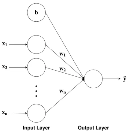
An ANN is a computational model that learns an approximation for a function given a series of inputs [49]. ANNs make use of artificial neurons for computations with synaptic connections between these neurons. These artificial neurons are typically of the Perceptron model introduced by Frank Rosenblatt in [50]. The Perceptron model consists of a neuron with synaptic connections, or weights, connected to its respective inputs. The neuron takes a weighted sum of its inputs and utilizes an activation function to obtain an output. An illustration of the Perceptron can be seen in Figure 2.1 as well as its respective calculation in (2.1).

ˆ y=f( n X i=1 xi∗wi+b) (2.1)

(30)

CHAPTER 2. BACKGROUND & RELATED WORK

Input Layer Output Layer

1

2

ˆ

1 2

Figure 2.1: Illustration of a Perceptron taking the weighted sum of its inputs and an additional bias term.

input to the neuron with its weights, w, and a bias term b, which is added on to offset the boundary decision of the algorithm. yˆ is the predicted output after the weighted sum of the inputs is sent through an activation functionf(). This activation function can be as simple as a threshold value to perform binary classification on an input. To update the weights of the model, a stochastic learning rule was employed as shown in (2.2).

w(t+1) =wt+η(y(i)−yˆ(i))x(i) (2.2)

t is the current training epoch of the model, η is the learning rate to adjust how much the weights would be changed, and y(i) _{is the ground truth observation for}

samplei. The Perceptron by itself could only perform linear separability between its inputs. Therefore, to handle problems that were not linearly separable, the

(31)

Multi-CHAPTER 2. BACKGROUND & RELATED WORK

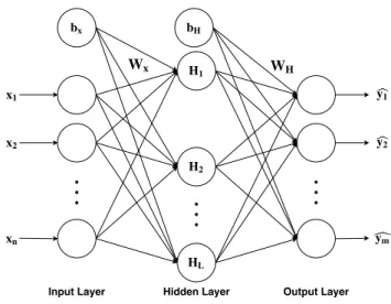
Layer Perceptron (MLP) was created. The MLP, as illustrated in Figure 2.2, makes use of a number of Perceptrons as artificial neurons in an ANN structure. The artificial neurons in this network create a hidden layer that takes the weighted sum of its inputs which is then sent to a nonlinear activation function. A set of common activation functions utilized in ANNs include sigmoid, hyperbolic tangent, or tanh, and Rectified Linear Unit (ReLU)) [51]. The equations for these activation functions can be seen in (2.3), (2.4), and (2.5).

1

2

Input Layer Hidden Layer Output Layer

1 ˆ1

2 ˆ

ˆ 2

Figure 2.2: Illustration of an MLP. In this architecture each progressive layer takes the weighted sum of its inputs.

sig(z) = 1 1+e−z (2.3) tanh(z) = e z₋_e−z ez₊_e−z (2.4) ReLU(z) =max(0,z) (2.5)

Through these activation functions the input’s value is transformed to be within a smaller number range. In the sigmoid activation function the values would be between

(32)

a range of [0, 1], while the tanh function sets the value to be between a range of [-1, 1]. Alternatively, the ReLU activation function keeps the original value if it’s equal to or above 0. These activation functions enable ANNs to learn more complex structures of its inputs. After taking the activated weighted sum of its inputs the network can perform a softmax activation function on the output layer to calculate which class the data is classified to be. The softmax operation can be seen in (2.6).

g(zc) =

ezc

Pc

i=1ezi

(2.6)

The softmax operation takes its inputs,zcand calculates the probability of which

class the input would be associated with. The highest probability would be considered the classified class for the given input. To configure the network such that it classifies its input correctly, a cost, or loss, function needs to be minimized as well as an adjustment to the weights in the network. A number of loss functions have been introduced, but in this work the log loss, or cross-entropy loss function, seen in (2.7), is focused on as it’s commonly used in image classification tasks.

Loss(i) =−log( e (oi_yi) Pc j=1eo i c ) (2.7)

In this loss function,o is the output of the last layer andyiis the correct class, or ground truth, of the sample i across all classes c. To minimize this loss the weights in a network are updated with learning rules, such as Stochastic Gradient Descent (SGD) through the backpropagation algorithm [20]. In this algorithm, each weight of the network is adjusted such that the loss would decrease over the training time. Through the use of multiple layers an ANN could learn to map its inputs to its selected outputs such that the data would be separated.

(33)

2.2

Convolutional Neural Networks

In this section CNNs are discussed as these networks are further explored in this work. Initially introduced in [52], CNNs are ANNs that consist of convolutional layers as well as dense, or Fully Connected (FC), layers used in MLPs. The convolutional layers used in these network are made up of filters with receptive fields, or filter sizes, that convolve over input images at a given stride. For each filter a single value is outputted by taking a weighted sum of its inputs. This allows for a similar operation to the FC layers, as a weighted sum of the inputs is taken, but in a sparse manner. Similarly to FC layers, a non-linear activation is typically applied to the output of a convolutional layer.

The sparse manner of the convolutional layer to the FC layer is illustrated through the calculation of the input weights of both the FC and convolutional layers. The comparison of the number of weights used in an FC layer as opposed to a convolutional layer is illustrated in (2.8) and (2.9) respectively.

Win =w∗h∗d∗N (2.8)

Win =K2∗F∗d (2.9)

The number of weights, denoted by Win, to be calculated in an FC layer would be equal to the product of the input’s width, height, and depth, denoted by w, h, and d, respectively, and the number of neurons in the FC layer, N. Alternatively, a convolutional layer would only require the product of its filter size, K, squared, the number of filters,F, and the depth of the input. This means for a given input image of dimensions 32×32×3 and 64 neurons, a FC layer would require 32∗32∗3∗64 = 196,608 input weights to be trained as opposed to a convolutional layer with 64 filters and

(34)

a filter size of 3× 3 requiring only 3 ∗3∗ 64∗ 3 = 1,701 weights to be trained. Additionally, unlike the FC layers, which require that the input image is flattened down to a vector form, convolutional layers can convolve over an input while retaining the given width, height, and depth allowing for spatial features to be preserved from the input.

In addition to convolutional layers, CNNs typically make use of pooling layers. Pooling layers are sub-sampling layers that decrease the dimensionality of an input. The most common pooling layers are max pooling layers and average pooling layers. In max pooling layers, the highest valued pixel, given a receptive field, is selected as the output. This operation occurs across the entire image to obtain a maximally activated output from an input. In contrast, the average pooling operation takes the average pixels in its receptive field. This allows for a low pass filtering operation on the input. This type of layer is commonly used after convolutional layers to transform and decrease the dimensionality of the input.

[52] illustrated how an end to end Convolutional Neural Network (CNN) could be trained with the backpropagation algorithm. In [1], the LeNet-5 CNN architecture, shown in Figure 2.3, was introduced as an improved version of the original design. This architecture consisted of 2 convolutional layers, 2 pooling layers, and 3 FC layers. Through the use of successive convolutional and pooling layers hierarchical features were able to be extracted from input images and then densely connected through the FC layers. This network was able to effectively learn representations from its input without the need for hand crafted features. It also paved the way for further research into CNNs.

2.2.1 AlexNet

Although LeNet-5 showed the initial potential of CNNs, CNNs were not widely adopted as they required large amounts of data to train on and were expensive in

(35)

Figure 2.3: The LeNet-5 shallow CNN architecture consisting of convolutional, pooling, and FC layers [1].

terms of resources due to the tuning process of the weights, or parameters, in their networks. It wasn’t until the introduction of AlexNet, depicted in Figure 2.4 that CNNs became popularized and widely used. AlexNet was merely a variant on the architecture of LeNet-5. It utilized convolutional, pooling, and FC layers just as LeNet-5 did. However, the authors of the AlexNet paper emphasized how depth played an important role in achieving high performance. They illustrated this by us-ing an 8 layer network, containus-ing 5 convolutional layers and 3 FC layers, as well as an additional 3 max pooling layers after some of the convolutional layers, that achieved state-of-the-art performance on the ImageNet dataset. This led to the beginning of the deep learning era as more researchers began to adopt deep CNN architectures to evaluate the effectiveness of these models on other aspects of computer vision.

Figure 2.4: The AlexNet CNN architecture consisting of multiple convolutional, pooling, and FC layers illustrating the impact of deep neural networks [2].

(36)

of techniques, such as utilizing ReLU activation functions, data augmentation, and dropout [53]. The method of using ReLU activation functions led to faster convergence as opposed to activation functions, such as sigmoid and tanh. While data augmenta-tion and dropout assisted in regularizing the network. All 3 of these techniques have since been utilized on various networks.

2.2.2 VGG

Following AlexNet was the Visual Geometry Group (VGG) Network which achieved state-of-the-art results on ImageNet surpassing AlexNet’s performance [54]. In these VGG networks, many 3×3 filter sizes were used as well as additional convolutional layers leading to variants of the architecture, such as VGG-16 and VGG-19, where the number after the hyphen denotes the number of layers not including the pooling layers. With the additional layers used in this architecture, the number of trained parameters increased as well as the number of resources needed to compute.

2.2.3 ResNet

As research into CNNs continued, researchers found that creating deeper networks didn’t necessarily always increase performance and in most cases would actually lead to decreased performance. This was due to the vanishing and exploding gradient problem [55, 56]. In the vanishing gradient problem, gradients calculated using back-propagation grow closer to 0 in the earlier layers due to saturation in the non-linear activation functions of these deep networks. This leads to little changes to the param-eters space in early layers. In contrast, the exploding gradient problem is where large gradients occur in the network leading to large changes in the parameter space. This can lead to an unstable network that does not converge properly. The ResNet ar-chitecture alleviates these problems through the introduction of residual connections. These residual connections are skipped connections from previous layers that map to

(37)

later layers enabling for identity mapping, depicted in Figure 2.5. More specifically, this skipped connection is an addition operation on a previous input and a current layer’s output. With the usage of these residual connections, the ResNet architec-ture was able to obtain state-of-the-art performance on numerous datasets, including ImageNet and the MS COCO datasets [57]. With these residual connections, much deeper networks could be created while enjoying an increase in performance rather than a degradation.

Figure 2.5: A ResNet residual block consisting of the use of skipped additive connectivity to alleviate the vanishing and exploding gradient problems [3].

2.2.4 DenseNet

Taking inspiration from networks with skipped connectivity, such as ResNet, the DenseNet architecture was formed [4]. This architecture enables for a large number of features to be extracted as all layers were connected through feature map con-catenation, as opposed to ResNet’s summing of feature maps. This leads to L(L₂+1) connections in a network as opposed toLconnections, whereLdenotes the number of layers in a network. In DenseNet architectures few filters are used to extract features for each layer, but as more features are concatenated to the entire amount of feature maps collected a substantial amount of salient feature can be extracted from these dense blocks, as shown in Figure 2.6.

As this dense connectivity can lead to a large amount of parameters, measures are taken to decrease the parameter space. The dense blocks of the network employed the

(38)

Figure 2.6: A DenseNet dense block consisting of the use of skipped concatenating con-nectivity to increase the number of features extracting in each layer [4].

use of bottleneck layers, introduced in [58, 59]. Bottleneck layers consist of applying 1×1 filters prior to 3×3 filters to decrease the number of parameters in the network as opposed to taking direct 3×3 filters on the input. In addition to the bottleneck layers, the number of feature maps between dense blocks were reduced. This meant that the intermediate, or transition, layers could output fewer feature maps to be fed into their next dense block. Through these techniques and the dense connectivity of the network design, a high performing model could be achieved with fewer parameters. This led to state-of-the-art performance surpassing the ResNet on datasets, such as ImageNet. Few networks were able to surpass DenseNet and of those that did many employed the use of large amounts of data augmentation, regularization, or an increased parameter space leading to higher resource utilization.

2.3

Random Weights in ANNs

In this section the use of fixed-random weights in ANNs is discussed. More specifically this section highlights the impact that the architecture has on the performance of a network with and without random weights. It additionally illustrates that comparable accuracies can be achieved in networks utilizing fixed-random weights on a number

(39)

2.3.1 The Importance of Architecture Design

A number of works have explored the usage of fixed-random weights. In this section a brief overview is given for a few of these works. In [60], the authors show that a shallow CNN with random weights and normalization can achieve comparable per-formance to a trained system on the Caltech-101 dataset [61]. The shallow networks consisted of convolution layers with 64 filters in the first layer and 256 filters in the second layer, both with 9×9 kernel sizes, that are then passed to a linear classi-fier. The performance was found to be sub-par in comparison to a trained network when evaluated on a dataset with greater labeled samples, such as the NYU Object Recognition Benchmark (NORB) dataset [13]. However, this work illustrates how random weights still enable features to be extracted from the input to enable fairly high performance.

The authors in [62] delve deeper into the work of [60]. They highlight the fact that random weights only result in a slightly worse performance than trained weights and explore the reasoning for this. The authors find that CNNs with random weights in their convolution and pooling layers can be frequency selective and translation invariant. Through a comparison of various trained and random CNN architectures, it’s found that there are cases where an architecture containing random weights can outperform a different architecture that has been trained. Therefore the authors conclude that the architecture alone plays an important role in key feature extrac-tion from inputs and that the learning algorithm used in these networks may not necessarily need to be the focus in yielding a high performance model.

2.3.2 Random Weights in DNNs Achieving Comparable Performance

In [5], the authors illustrate the usage of fixed-random weights in image reconstruc-tion, synthesizing textures, and utilizing neural style transfer [6]. They make use of a VGG-19 CNN as their chosen network and replace the maximum pooling layers of the

(40)

architecture with average pooling. All weights of the architectures were initially set to random values from a Gaussian distribution with zero mean and a standard deviation of 0.015. After random weights were initialized they stack the network layer by layer with new random weights in a greedy manner. In their new constructed network, they first sample images with an array of random weight combinations to find a set that minimizes the loss for one layer. They then repeat the process until the network leads to ideal random weights. A comparison of the reconstructions of images for the randomized VGG, denoted by ranVGG, and a fully trained VGG net on ImageNet, denoted by VGG, can be seen in Figure 2.7.

Figure 2.7: Reconstructions of 3 images when utilizing a fully random VGG net and a fully trained VGG net [5]. The visualization from the pool5 layer exhibits certain features learned in the trained net that inhibits reconstruction.

A clear difference can be seen perceptually between the fully random and trained VGG nets for the pool5 layer. The image reconstruction for the random network is shown to be more visually appealing. However, the authors take a greedy approach in constructing the ranVGG network. Additional experiments from the author show that textures can be generated as shown in Figure 2.8. Additionally, neural style transferred images can be generated as shown in Figure 2.9.

(41)

Figure 2.8: Generated textures from several images when utilizing a fully random VGG net and a fully trained VGG net [5]. In this figure each row corresponds to a convolutional layer in the random VGG net while a comparison is made between the 4th convolutional layer of both the trained and random nets.

A difference can be seen between both the images of the textures and the neural style transferred images. For example, in the texture images, Figure 2.8, the conv4 1 of the random VGG for the floors shows textures that are not as sharp as trained conv4 1. However, across the other textures, this is visually unnoticeable. Although the textures are not as distinct, in comparison to the trained net, the random net is

(42)

Figure 2.9: Neural style transfer of images when utilizing a fully random VGG net and a fully trained VGG net [5]. The first row depicts the original image, while the second and third rows show the random VGG net and trained VGG net’s content images with the applied style transfer. Note: The reference [13] in this image refers to [6]’s paper.

still able to extract textures from the given input.

This can be additionally seen in the neural style transferred images as the trained net depicts sharper more noticeable changes in the transferred content image for Der Schrei. However, this is not as visually noticeable when utilizing the other style images. These transferred content images are still able to obtain features from both style and content as the architecture enables for various features to be extracted from the input.

To explore the impacts of random weights even further, the authors in [7] exper-iment on training only portions of the weights in CNNs while leaving the untrained weights to their initialized random values. Many previous works explore the usage of layers containing random weights, but this work explores the use of layers containing a mixture of trained and random weights. They observe the effects of training con-volutional layers with a percentage of trained filters while the rest are left untrained. Additionally, these experiments included tests on leaving only a value of k filters trained per convolutional layer. For these experiments the FC layers of each architec-ture consisted of weights that were trained. These experiments on both the Canadian

(43)

Institute for Advanced Research (CIFAR)-10 [8] and CIFAR-100 [8] datasets can be seen in Figure 2.10.

Figure 2.10: Experiments utilizing a percentage and a k amount of trained weights in deep CNN architectures. The white area indicates the percentage of weights trained, while the gray area indicates training on only k number of filters per convolutional layer. The blue line indicates the rest of the weights in the layer were left untrained, while the green line indicates the rest of the weights in the layer were zeroed out [7].

The architectures used in this experiment, from left to right in Figure 2.10, include DenseNet with a depth of 100 and a growth rate of 12, Wide ResNet (WRN) [63] with 28 layers and a widen factor of 4, VGG-19, and AlexNet. The experiments show that each architecture was able to achieve fairly high performance even with a large portion of weights left random. Additionally, across many of the architectures the random weights a small increase in performance over leaving the weights zeroed out. It is also seen that even learning a subset ofk filters while leaving the rest untrained can lead to fairly high performance most notably in the DenseNet architecture.

Unfortunately, in this experiment the authors fail to illustrate the accuracy achieved by a fully trained model after the 10 epochs of training. It’s also unclear if a greater number of training epochs would have substantial effects on the accuracies achieved by these networks with random weights. Fortunately, the authors conduct an

(44)

experi-CHAPTER 2. BACKGROUND & RELATED WORK

ment where they train the WRN model and DenseNet model for 200 and 300 epochs, respectively, as shown in Table 2.1.

Table 2.1: Performance achieved when learning only a fraction of filters for the CIFAR-10 dataset for training epochs of 200 on WRN and 300 on densenets. Eff. Params indicates the number of trained parameters, while * indicates the performance when the parameters for random weights were zeroed out [7].

Method Fraction Eff. Params x 106 Perf Perf* WRN 0.1 3.66 94.12 91.53 WRN 0.4 14.6 95.75 95.49 densenets 0.1 0.09 88.73 82.11 densenets 0.4 0.3 93.33 92.46

In this experiment the WRN and DenseNet models were compared with small fractions of trained convolutional weights and large fractions of random or zeroed out convolutional weights on the CIFAR-10 dataset. It can be seen that the random weights are more influential when a small fraction of weights (0.1) is trained. How-ever, the experiments of zeroing out the weights for the 0.4 trained fraction amount indicates that the random weights only assist the performance marginally (<1%). Another experiment comparing the two networks for 200 and 300 epochs of training, respectively, on the CIFAR-10 and CIFAR-100 datasets can be seen in Figure 2.11.

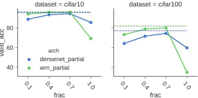
This figure illustrates how even learning 70% of the weights is a substantial amount in enabling for a model that reaches performance comparable to its respective trained equivalent for both the CIFAR-10 and CIFAR-100 datasets. The authors evaluate on one more dataset, namely the Tiny-ImageNet dataset [64]. This dataset is an alternative to the ImageNet dataset and consists of 200 classes with 500 training and 50 validation images for each class. Each image is of RGB color and size 64×64. The experiments conducted on this dataset consisted of training only the WRN model for 45 epochs with an initial learning rate of 0.1 which was decreased by a factor of 10 every 15 epochs. The result of this experiment is shown in Table 2.2.

(45)

Figure 2.11: The WRN and DenseNet networks compared on both the CIFAR-10 (left) and CIFAR-100 (right) datasets at various training fractions per convolutional layer. Green and blue solid lines indicate networks with a fraction of trained weights and the rest left random. Green and blue dashed lines indicate the performance of the WRN and DenseNet networks with trained weights. Note: when frac = 1.0, this is actually when only a single filter is trained per convolutional layer [7].

Table 2.2: Performance on the Tiny-ImageNet dataset using the WRN model with various percentages of trained weights [7].

% Params Top-1 Accuracy (%) # Params

10 21.75 .83M

40 30.13 2.58M

70 33.22 4.33M

100 35.54 6.1M

while all other weights are left random high accuracies can be achieved. This work illustrates how much of an impact the architecture can have on the performance of deep CNNs as initially discussed in [62]’s work.

Overall, the research into the field of fixed-random weights in ANNs illustrates how these networks may not necessarily need to be fully tuned. However, the architectural design of the ANN plays an important role in extracting meaningful features from the input. Additionally, a purely random network can yield comparable performance in some cases to fully tuned networks. This brings into question, though, of how many

(46)

parameters need to truly be tuned in a network? It’s not necessarily true that all parameters need to be tuned as a purely random network illustrates the impact of the architecture. On the other hand, if only portions of a network are tuned then a network can still reach comparable performance to its respective trained model.

2.4

Random Projection Networks

Aside from the works discussed above, many other works highlight the use of random weights in ANNs. In the work of [40], the extreme learning machine (ELM) architec-ture is introduced. This architecarchitec-ture is a feed-forward architecarchitec-ture, similar in design to a single hidden layer MLP, that makes use of random projection from its inputs to a hidden layer and conducts training on the output layer weights. A similar concept is utilized in the form of recurrent ANNs. This concept, better known as reservoir computing, is explored in two works by [41] and [42] through the introduction of the Echo State Network (ESN) and Liquid State Machine (LSM), respectively. In both works the input to hidden layer weights are left as a random projection along with a reservoir layer containing recurrent neurons with random weights and connectivity to other neurons. Through the random nature of the reservoir layer, feedback signals are introduced from temporal inputs enabling for an innate form of fading memory. Similarly to the ELM, the ESNs and LSMs are trained only on their output layer weights.

2.4.1 ELM

The ELM approach to fixed-random weights has become increasingly adopted in the literature [65]. The ELM architecture is a shallow feedforward ANN that makes use of two fully connected (FC) layers, similar to that of the structure of an MLP illustrated previously in Figure 2.2. In this architecture, the input to hidden layer weights are

(47)

a larger more separable space as the hidden layer nodes in the network are typically greater than the number of input nodes. The hidden to output layer weights are then trained using an alternative training paradigm to SGD, namely taking the MPP [39] of the output weights given all training samples. By taking the inverse of a matrix a least squares solution can be calculated. However, the matrix must be square to take the inverse. Unfortunately, it is rare for this to occur given most data. Therefore, by using the MPP, a least squares approximation of the output weights can be computed by taking the generalized inverse of the matrix. The evaluation of the output layer’s weights in an ELM is calculated using (2.10), (2.11), and (2.12).

H†= (HTH+λ_I)−1HT (2.10)

Wout =H†y (2.11)

ˆ

y=HWout (2.12)

Initially the MPP of H is taken using (2.10), where H† is the MPP of H, H is the output of the hidden layer, and λ acts as a regularization term multiplied by an identity matrix,_I. Equation (2.11) then highlights the calculation of the least squares approximation. In this equation the output weight matrix, Wout, is calculated by multiplying H† by y, which is the ground truth labels. Once the output weights are calculated, the output predictions, ˆy, are calculated in (2.12) by multiplying the output of the hidden layer and the output weights. The output predictions are then used to compare to the ground truth labels to evaluate the network’s performance.

(48)

2.4.2 Random Vector Functional Link Network

Prior to the introduction and popularization of the ELM, there was another network that introduced random projection, namely the Random Vector Functional Link Neu-ral Network (RVFL) [46]. In this network, hidden layer nodes were called enhance-ment nodes. The weighted connection between the input and enhanceenhance-ment nodes were set to fixed-random values during the training process while the output weights were trained. The training paradigms used in this network would consist of either a gradient based approach or training in one step through the utilization of the MPP. Many similarities can be seen between the ELM and this network, however, this net-work makes use of an additional link, or skipped connection, from its input to its output. This skipped connection was a concatenation of the input-to-output weights to the enhancement-to-output weights. Therefore, in the calculation of the MPP of the output layer’s weights of the network, theHmatrix of (2.10) would consist of the additional initial inputs. Through the use of this skipped connection, the RVFL was shown to be able to approximate functions well in comparison to a normal MLP.

An in depth evaluation of the skipped connection was studied in [47] for this network. The authors tested this connection on 121 datasets from the UCI machine learning repository [66] to assess the direct input-to-output connection. They found that the connection led to an increase in accuracy for the datasets when compared to an RVFL lacking this connection. They concluded that this link acted as a regularizer for the randomized weights and enhanced the performance of the network.

The authors in [48] introduce the Convolutional Random Vector Functional Link Neural Network (CRVFL), which is a combination of the concepts used in CNN archi-tectures and the RVFL architecture. This architecture made use of a convolutional layer, an average pooling layer, a normalization layer, and a FC layer, as well as the input-to-output skipped connection, to perform visual tracking. Similarly to the

(49)

random. Training only occurred on the output layer and the training paradigm con-sisted of a recursive least squares approach as visual tracking was a task that occurred over time as opposed to image classification which is purely spatial. Using this ar-chitecture, the authors showed results on a 51 video sequence of tracking objects and showed comparable performance to CNN backpropagation methods.

2.5

Tensor Decomposition

In many ANNs today the flow of data is typically represented in terms of vectors or matrices. For example, an MLP with a single hidden layer ofH neurons has weighted connections from its input to a successive layer. The H neurons are represented in the form of a vector, while the weighted connections are represented in the form of a matrix. In mathematics there is another method of representing these matrices through the use of tensors. Tensors are multidimensional arrays where each dimension is a vector space [67]. The dimension of a tensor goes by many names, such as its order, number of ways, or number of modes [67]. These terms are used interchangeably in the literature, however, clarification is given to ensure readability of this work. A clear example of the dimensionality of tensors can be seen in Figure 2.12.

Vector

Matrix

3rd Order Tensor

2nd Order Tensor

1st Order Tensor

Figure 2.12: Illustration of tensors in varying orders, or dimensions.

In this figure tensors in their respective dimensions are shown. A tensor of d = 1 is a vector or 1st order tensor, a tensor of d = 2 is a matrix or 2nd order tensor, a

(50)

tensor of d = 3 is a 3rd order tensor, and lastly a tensor of d = N is an Nth order tensor. Additionally, a tensor of d = 0 is merely a scalar. In this work, tensors of order 3 or higher are denoted with bold upper-case letters, such as X, as opposed to matrices denoted by italicized upper-case letters, such as X. Vectors are denoted by lower case scripted letters, such as a.

Decomposing data, or compressing it, to a smaller or approximate form is ben-eficial as it decreases the dimensionality of the data. Many applications, such as signal processing [68], image compression [69], machine learning [70], etc., require the use of compression techniques to decrease the number of resources used. Therefore, the tensor decomposition has become popularized as it presents effective methods in decomposing high dimensional data [67].

In order to understand tensor decompositions, it’s important to first understand matrix decomposition. In matrix decomposition problems, an initial matrix X is approximated by a low-rank modelM. M is calculated by taking the sum of a subset of rank-one matrices as shown in (2.13).

X ≈M =

r

X

l=1

al⊗bl =AB|= [AB] (2.13)

The outer product, denoted by ⊗, of vectors a and b is taken with l as the index into the vectors across allr, which is the total number of ranks. This is equivalent to

AB|_{, where}_B| _{is the transpose of B.}

Under tensor representations, an Nth order rank-one tensor can be represented as the outer products of its respective 1st order tensors, or vectors. Rank-one tensors refer to an Nth order tensor that can be decomposed into the outer product of

N 1st order tensors. For example, suppose we have a rank-one tensor of order 3,

(51)

tensors, a∈_Rm_,_b _∈

Rn, and c∈Rp, as shown in (2.14).

T=a⊗b⊗c (2.14)

Aside from the example of a rank-one tensor, the rank of a tensor is defined as the summation of the minimum number of rank-one tensors whose summation produce the original tensor [71]. However, determining the rank required to produce an original tensor is found to be an NP-hard problem [72, 73]. Although, determining the rank is an NP-hard problem, the use of tensor decomposition still holds benefits over matrix decomposition as it extends to higher orders.

To gain an understanding of tensor decomposition, one of the more well known and original tensor decomposition is the canonical polyadic (CP) decomposition [74]; also known as the CANDECOMP/PARAFAC decomposition [75, 76]. In this method of decomposing a tensor, a tensor is approximated by respective rank-one tensors. Figure 2.13 illustrates an example of CP decomposition on a 3rd order tensor, T, which is approximated by rank-one tensors, a, b, c. Equation (2.15) presents the calculation for an Nth order tensor.

T

≈

a₁ c₁ b₁ a₂ c₂ b₂ a_r c_r b_r

+

Figure 2.13: Illustration of a tensor decomposition in which an input Tis approximated by the summation of rank-one tensors. These rank-one tensors are calculated from the outer product of 1st order tensorsa,b, andc.

T≈

r

X

l=1

al⊗bl⊗cl = [ABC] (2.15)

(52)

a component and the matrices [ABC] are referred to as factor matrices that describe the 3rd tensorT. By summing the rank-one tensors across rranks the original tensor

T can be approximated. In contrast to matrix decomposition, tensor decomposition holds the benefit of enabling for less rigidness in unique solutions. The matrix decom-position to approximate a low-rank model typically doesn’t hold a unique solution unless additional constraints are made to the matrices. For example, various matri-ces A and B can enable for an approximate model M to be formed [77]. However, tensor decomposition can approximate a low-rank model with less rigid constraints as deterministic approaches can be made to either compute or enable uniqueness in the decomposition [71]. As the mathematical proofs for this uniqueness is out of the scope of this work, the readers are referred to [71] for additional information on this topic. Additionally, a survey on