Turun kauppakorkeakoulu • Turku School of Economics
Bachelor’s thesis
x Master’s thesis
Licentiate’s thesis
Doctor’s thesis
Subject Accounting and finance Date 6.8.2019
Author Marjut Soininen Student number 509850
Number of pages 92
Title Factor selection for multifactor models: Bayesian model averaging approach
Supervisors Prof. Mika Vaihekoski and M.Sc. Valtteri Peltonen
The optimal set of factors for multifactor model has been under discussion in the previous decades. Research has focused mostly on the Fama-French models and the inclusion of some additional factors. Moreover, the research has been mostly limited to fundamental factors and traditional hypothesis testing based on p-values. In this thesis, factor selection is done with the Bayesian approach, where
factors are evaluated based on their posterior probabilities of inclusion rather than their p-values.
Twelve factors are included in the algorithm as potential factors and all possible combinations of these factors are evaluated simultaneously. The model with the highest posterior probability is then chosen. The specific method used is Bayesian model averaging (BMA), which has received good results in previous studies of stock market factor selection. The significance of macroeconomic fac-tors besides fundamental facfac-tors is examined as well. Finally, the predictability ability of the con-structed multifactor model is compared to the Fama-French models and CAPM.
The time period of research is from 2007 to 2018, where 2007−2016 is the in-sample and
2017−2018 the out-of-sample period. All NYSE, AMEX and NASDAQ stocks, which have the rele-vant data available, are included in the research. The following six factors have the highest posterior probability: market premium, size, value, momentum, the changes in long-term interest rate, and oil price change. These factors form the BMA multifactor model. The out-of-sample results show that the BMA multifactor model constructed here has the lowest Mean Squared Error (MSE) value, so it can predict stock returns out-of-sample better than Fama-French models or CAPM. The results are robust for the test portfolios used.
The results are in line with previous findings that the Bayesian approach is a useful tool for factor selection. Widely examined fundamental factors (market, size and value premium) as well as mo-mentum factor still seem to have some predictability ability in the US, and since inclusion of macro-economic factors improves the predictability of model, they should be examined more alongside fun-damental factors in the literature.
Key words Bayesian model averaging, factor selection, multifactor model, US stock market Further
Turun kauppakorkeakoulu • Turku School of Economics
Kandidaatintutkielma
x Pro gradu -tutkielma Lisensiaatintutkielma Väitöskirja
Oppiaine Laskentatoimi ja rahoitus Päivämäärä 6.8.2019
Tekijä Marjut Soininen Matrikkelinumero 509850
Sivumäärä 92
Otsikko Monifaktorimallin faktoreiden valinta bayesilaisella keskiarvoistamisen menetelmällä
Ohjaajat Prof. Mika Vaihekoski ja KTM Valtteri Peltonen
Monifaktorimallit ja faktoreiden optimaalinen valinta ovat kiinnostaneet tutkijoita viime vuosikymmeninä. Tutkimus on keskittynyt lähinnä Fama-French-malleihin ja niihin yhdisteltäviin faktoreihin. Lisäksi tutkimus on rajoittunut suurimmaksi osaksi fundamentaalisiin faktoreihin ja perinteiseen p-arvoihin perustuvaan hypoteesien testaamiseen. Tässä tutkielmassa faktoreiden valinta
suoritetaan bayesilaisella menetelmällä, jossa faktoreita arvioidaan p-arvojen sijaan
posterioritodennäköisyyksillä. Kahdentoista potentiaalisen faktorin kaikki mahdolliset yhdistelmät arvioidaan perustuen näihin todennäköisyyksiin ja malli, jolla on korkein posterioritodennäköisyys, valitaan. Käytetty menetelmä on bayesilainen mallikeskiarvoistaminen (Bayesian model averaging, BMA), jolla on saavutettu hyviä tuloksia aiemmissa faktoreiden valintaan liittyvissä tutkimuksissa. Lisäksi makroekonomisten faktoreiden merkitystä tutkitaan. Muodostetun multifaktorimallin ennustuskykyä verrataan Fama-French-malleihin ja CAPM:iin keskineliövirheellä (MSE) mitattuna.
Tutkimus suoritetaan USA:n markkinoilla 2007−2018, jossa otosikkuna on 2007−2016 ja otoksen
ulkopuolinen ikkuna 2017−2018. Kaikki NYSE:n, AMEX:in ja NASDAQ:in osakkeet, joista on
tarvittava data saatavilla, sisällytetään tarkasteluun. Seuraavilla kuudella faktorilla on korkein posterioritodennäköisyys ja jotka siten sisällytetään BMA monifaktorimalliin: markkinapreemio, koko- ja arvofaktorit, momentum, pitkien korkojen muutos ja öljyn hinnan muutos. Otoksen ulkopuolinen testaus osoittaa, että BMA monifaktorimallilla on pienin keskineliövirhe, joten se pystyy ennustamaan osaketuottoja paremmin kuin Fama-French-mallit tai CAPM. Tulokset ovat robusteja testiportfolioiden valinnalle.
Tulokset ovat linjassa aiempien tutkimusten kanssa ja osoittavat, että BMA menetelmä sopii hyvin faktoreiden valintaan. Lisäksi tulosten mukaan paljon tutkitut fundamentaaliset faktorit näyttävät edelleen selittävän osaketuottoja USA:ssa. Makroekonomisten muuttujien sisällyttäminen parantaa myös mallin ennustekykyä ja niitä tulisi siten tutkia enemmän fundamentaalisten faktoreiden ohella.
Asiasanat bayesilainen tilastotiede, faktorivalinta, monifaktorimalli, USA:n osakemarkkinat Muita tietoja
FACTOR SELECTION FOR MULTIFACTOR
MODELS
Bayesian model averaging approach
Master´s Thesis in Accounting and Finance
Author: Marjut Soininen Supervisors: Prof. Mika Vaihekoski M.Sc. Valtteri Peltonen 6.8.2019 Turku
The originality of this thesis has been checked in accordance with the University of Turku quality assurance system using the Turnitin Originality Check service.
1 INTRODUCTION ... 9
1.1 Background and motivation ... 9
1.2 Research questions and limitations ... 11
1.3 Structure of the thesis ... 13
2 MARKET PREMIUM AND OTHER RISK FACTORS IN MULTIFACTOR MODELS ... 14
2.1 Efficient Market Hypothesis ... 14
2.2 Pricing anomalies ... 16 2.2.1 Size Effect ... 17 2.2.2 Value effect ... 20 2.2.3 Momentum effect ... 22 2.2.4 Macroeconomic factors ... 23 2.2.5 Multifactor models ... 26
3 BAYESIAN APPROACH IN MULTIFACTOR MODELS ... 28
3.1 Bayesian framework ... 28
3.1.1 Advantages and limitations ... 28
3.1.2 The Bayesian theorem... 32
3.1.3 Prior information ... 34
3.2 Bayesian model averaging (BMA) for factor selection ... 38
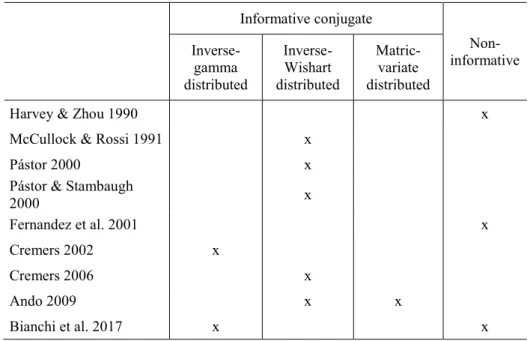
3.3 Previous findings and literature ... 43
3.3.1 Previous literature on factor selection with the Bayesian model averaging method ... 43
3.3.2 Previous literature on factor selection with other Bayesian methods ... 45
4 DATA AND RESEARCH METHODOLOGY ... 51
4.1 Data ... 51
4.2 Methodology ... 55
5 EMPIRICAL RESULTS ... 61
5.1 Descriptive analysis... 61
5.2 Results from Bayesian model averaging ... 66
5.3 Performance of BMA multifactor model by out-of-sample forecasting ability ... 70
6 CONCLUSIONS ... 81 REFERENCES... 83
Table 1 Prior types in different papers ... 38
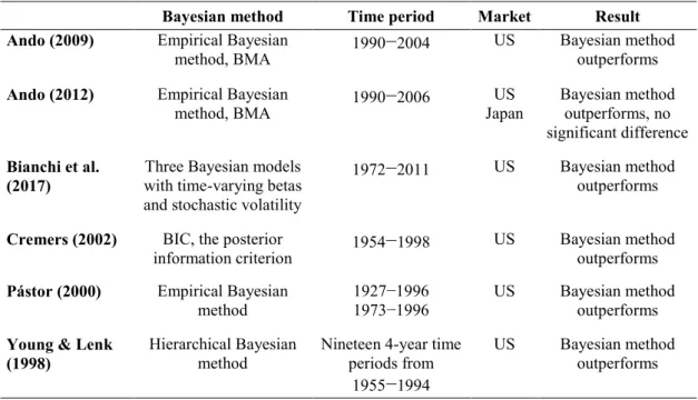
Table 2 Previous studies that compare the standard p-values based and Bayesian methodology in testing multifactor models ... 50
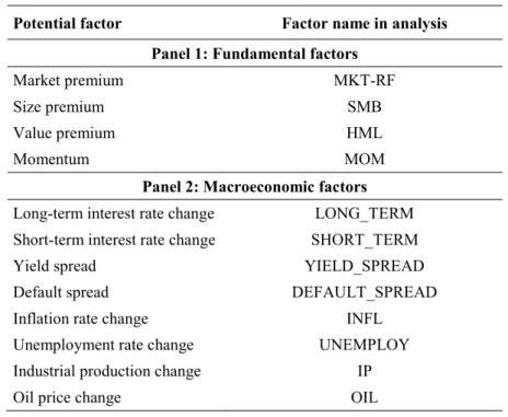
Table 3 BMA factors included in the empirical research ... 51
Table 4 Industry portfolios and their names in the analysis ... 52
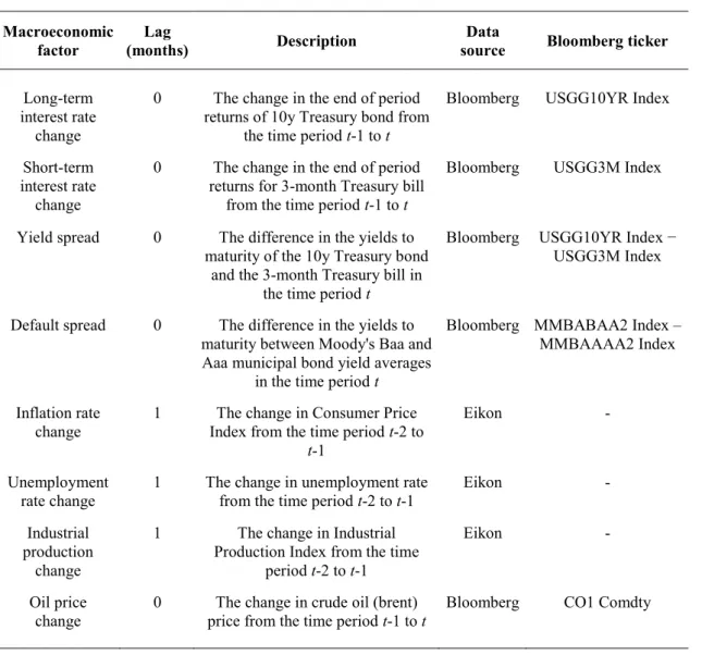
Table 5 The sources and definitions for macroeconomic factors ... 55
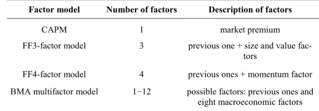
Table 6 An overview of the factor models under comparison ... 57
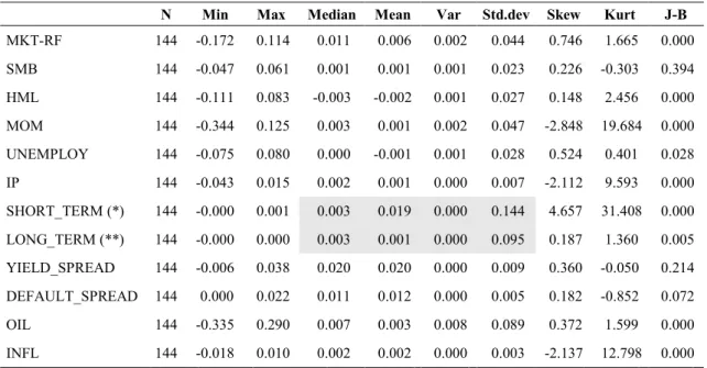
Table 7 Descriptive statistics for potential fundamental and macro-economic factors ... 62
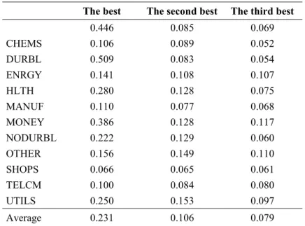
Table 8 Posterior probabilities for the best models in every industry and for the individual factors ... 67
Table 9 Posterior probabilities for the second and third best models ... 68
Table 10 Beta coefficients for the all factors in multifactor models in every industry ... 71
Table 11 Expected factor realizations for 2017−2018 and average values ... 72
Table 12 The expected returns and MSE values with 10-year rolling factor realizations for all factor models ... 76
Table 13 The expected returns and MSE values with previous month´s factor realizations for all factor models ... 77
Table 14 MSE values for ten size portfolios ... 80
LIST OF FIGURES
Figure 1 Premiums for fundamental factors in 2007−2018 ... 641
INTRODUCTION
1.1
Background and motivation
The characteristics of stock returns and portfolio selection are some of the core interests in finance and have always been of interest to both practitioners and academics. One of the most crucial problems is finding a specific model, which adequately expresses the dynamics of asset returns. (Ando 2009, 556; Tsai et al. 2010, 110.) While there are nu-merous papers documenting predictability, there is little consensus across these articles on what the important variables are (Cremers 2002, 1223).
Modern portfolio theory, developed by Markowitz (1952), was one of the first and most important steps in understanding stock behavior (Rubinstein 2002, 1041). Since then various factors have been found and different models tested over the years. In the 60s many researchers focused on the Capital Asset Pricing model (CAPM), which is based
on Markowitz’s theory and was developed independently by Sharpe (1964), Lintner
(1965) and Mossin (1966). The main point in the CAPM was that stock returns can be explained with only one factor, the market premium, to which different assets have dif-ferent loadings (beta coefficients).
The CAPM equilibrium has been criticized since the model was introduced. Many researchers have recognized the problems in testing the model that are caused by the strict
assumptions behind the model. One of the most known critics is the so-called Roll’s critic,
which states that only the efficiency of the market portfolio can be tested with the CAPM and it has no implications on the return-risk-relationship (Roll, 1977). Later Fama and French (2004) received similar results.
Besides the testing errors, the CAPM’s assumption of a one risk factor has been widely
questioned in past decades. Many researchers have found pricing anomalies that generate new risk factors. Some of the most known pricing anomalies are size effect, value effect and momentum effect. (Bender et al. 2013, 4.) Because of these findings, finance re-searchers have focused lately on the multifactor models that consist of various risk char-acteristics and solve the portfolio choice problem with models far more sophisticated than the mean-variance framework of Markowitz or the CAPM one factor model (Ando 2009, 551). Fama and French (1992; 1993; 2004) have made pioneering research among risk factors and developed perhaps the best-known multifactor models.
Researchers and financial professionals mostly agree nowadays that there is more than one risk factor that affects stock returns. A common view however, has not been reached on how many factors and which ones should be included. Some researchers, for example, have suggested that the size effect has disappeared in the last few years although it is still widely used in many funds by practitioners (Ang 2014, 229).
Many different factors have been considered as a component of multifactor models. These factors can be divided into fundamental, macroeconomic and statistical factors. (Connor 1995, 42.) The question now is how to combine these potential factors to achieve the most optimal multifactor model, that is, the combination of factors that explains stock returns most accurately and can thus be used in predicting the stock returns.
The common way to evaluate different factors and risk premiums is to add one or more new factors to the Fama-French models. For example, Carhart (1997) adds a momentum premium to the FFfactor model and reaches better results compared to the original 3-factor model. However, this approach assumes that the combination of 3-factors is fixed and evaluates only one model per time. This method can lead to the better model being compared to universal multifactor models but does not technically focus on factor selec-tion as the set of factors is picked in advance.
To get the most optimal multifactor model all the existing factors and models should be included in testing. Obviously, it is not possible to include all the factors since there are thousands of them in existing literature alone and many of them are strongly correlated with each other. Some methods have been developed to test multiple combinations of factors, which leads us a little bit closer to factor selection analysis and the most optimal multifactor model. (Fernandez 2001, 381.)
One method is to utilize the Bayesian approach, where the main idea is to first select a set of possible factors and then evaluate all the possible combinations of these factors based on their prior and posterior probabilities (Ando 2009). The prior probability refers to the probability, in which the factor is included in the optimal model based on previous knowledge, views, or specific distribution. These probabilities are then updated with the new data, which results in the posterior probabilities. (Puga et al. 2015, 277.)
With these methods it is possible to examine the common problem of finding the most relevant factors and construct a model, where the number of factors is restricted. Bayesian methodologies have several advantages compared to traditional hypothesis testing (for example, the Fama-MacBeth approach). For example, they take into account parameter uncertainty, as they allow a wide range of prior distributions and evaluate all possible combinations of factors to calculate posterior probabilities. (Bianchi et al. 2017, 111.)
Common Bayesian methods however do not take into account model uncertainty, which is another possible problem in classical hypothesis testing. Barnard (1963) was the first one to mention the idea of combining models in statistical literature. Later some other
approaches were developed, like Akaike’s information criterion (AIC). (Hoeting et al.
1999, 384, 398.) Lately, more attention has started to be paid to applying model combin-ing to Bayesian methodology. This has resulted in the Bayesian model averagcombin-ing ap-proach (BMA), which takes into account both parameter and model uncertainty.
Although factor selection is a very important part of constructing multifactor models, previous literature provides very little guidance on it. There is no consensus among re-searchers about what the best factors in predicting stock returns would be. In this thesis, the problem of selecting relevant factors is examined and therefore a set of factors is not decided beforehand. Instead, many fundamental and macroeconomic factors are recog-nized as potential factors and the final set of optimal factors is formed from among them with the Bayesian model averaging method. Macroeconomic factors are included in the study because the existing empirical research has lately mostly focused only on funda-mental factors.
Bayesian model averaging can be used in two ways. First, it can be used to find the most optimal multifactor model among all the competing models based on the posterior probabilities of models. The model that has the highest posterior probability is selected.
Second, the number of competing models can be reduced with the use of Occam’s
win-dow and the remaining models can then be used as portfolio weights based on the poste-rior probabilities of models. (Steel 2011, 33.) This second approach uses all the competing models and greatly reduces model uncertainty.
Bayesian methodology is widely known among statisticians, and has been applied to
many different purposes, but it’s implications on the factor selection problem in
multi-factor models are relatively unknown and a limited number of previous researches are available on the subject. Especially few research papers are available on the Bayesian model averaging approach, although the results have been promising. Moreover, the BMA method has many advantages compared to other, more classical, factor selection approaches. (Young & Lenk 1998; Berger et al. 2001; Fernandez et al. 2001; Ando 2009.) It is interesting to examine how the Bayesian model averaging method works in factor and model selection at the present time and if it is possible to construct better and more accurate multifactor models than the universal FF3 and FF4 factor models.
1.2
Research questions and limitations
The purpose of this thesis is to consider the different factors that have an impact on stock returns and examine the problem of selecting the most optimal factors. The possible fac-tors included in testing are based on the existing literature. The factor selection is done with the Bayesian model averaging approach. The research questions are formed as fol-lows:
Which factors are important for explaining stock returns in the Bayesian model averaging approach and should therefore be included in the optimal multifactor model?
and
Does this Bayesian multifactor model predict stock returns out-of-sample better compared to benchmark models?
The first question is examined with the Bayesian model averaging technique and the
method is constructed mostly based on Ando’s (2009) article about Bayesian portfolio selection. In Ando’s research two different Bayesian approaches are utilized and
com-pared to the mean-variance portfolio selection style. However, in this thesis only one Bayesian construction method is used, the Bayesian model averaging method.
Factor selection is done in-sample and as a result, the optimal multifactor model ac-cording to the Bayesian method is achieved. Other competing models are also briefly analyzed, but only the best model is selected to the out-of-sample testing. In other words, the second method of using Bayesian model averaging, where all the individual models are included in the optimal model based on the weights determined by posterior proba-bilities, is not used in this thesis. This choice can be made because results show that the difference in the posterior probabilities between the best and second-best models is rela-tively large. Therefore, focusing solely on the best model does not significantly reduce the reliability of the study (Steel et al. 2011, 33).
The second research question relates to the usefulness of constructed multifactor mod-els and their ability to predict stock returns compared to benchmark modmod-els. The out-of-sample performance of the formed Bayesian multifactor model is compared to the one factor model (CAPM), and two multifactor models, the FF3-factor model and FF4-factor model. The performance is examined using the mean squared error (MSE), which calcu-lates the difference between the actual returns and the expected returns of the factor model.
Theoretically, in the Bayesian model averaging method, an unlimited number of fac-tors and models can be considered. In this thesis the number of potential facfac-tors is re-stricted to four fundamental and eight macroeconomic factors that have strong academic relevance and logical, but not always rational, reasons for their existence in the markets. All other factors are left to future research.
The testing of the competing factor models is done for the portfolios of stocks rather than for individual assets. The reason for this is that returns need to be stationary in the sense that they have approximately the same mean and covariance and individual stocks are usually very volatile. (Ericsson & Karlsson 2003, 6.) Twelve industry portfolios are therefore used for testing the hypothesis, which is a common method in the literature.
The research is done using U.S. data and all the NYSE, NASDAQ and AMEX stocks, that have the relevant historical data available, are included. The time period for the
in-sample factor construction is ten years, 2007−2016. Monthly data is used, so 120 obser-vations are included in each industry portfolio in the BMA factor selection. The time
period for out-of-sample testing is two years, 2017−2018.
1.3
Structure of the thesis
Section 2 focuses on the theory behind the multifactor models. First, the efficient market hypothesis is introduced and after that the most relevant stock market anomalies and fac-tors. Finally, multifactor models, including the APT and Fama-French models, are dis-cussed briefly based on these factors.
The next section, Section 3, concentrates on the Bayesian approach. First, the basic idea behind the model is introduced and its implications on factor selection are discussed, as well as the advantages and disadvantages of the model and prior information. Second, the Bayesian model averaging method is introduced, and the formulas derived. In addi-tion, the existing relevant literature from the topic and previous findings are discussed in the end of Section 3.
Section 4 focuses on representing the data and methodology that is used for the empir-ical research of this thesis. The results are finally shown in Section 5, first from the Bayes-ian model selection and then the performance of the model compared to the benchmarks. A robustness check is made in the end of Section 5. The conclusions are summarized in Section 6 after which references are shown.
2
MARKET PREMIUM AND OTHER RISK FACTORS IN
MULTIFACTOR MODELS
2.1
Efficient Market Hypothesis
The Efficient Market Hypothesis (EMH) is a theory whereby the securities market is ef-ficient, which means that share prices always fully reflect all available information. The theory assumes that when new information arises, it spreads very quickly and affects share prices without delay. (Malkiel 2003, 59.) Therefore, in efficient markets, fluctuation in share prices should not appear if there is no new information available and stocks should always trade at their fair value on stock exchanges.
EMH was presented by Fama (1970) and it is based on previous findings of investors’
rationality and the idea of a “random walk”. Random walk describes the scenario where all subsequent price changes are unrelated to previous prices. The logic of the theory is
that if all the information is immediately reflected in share prices, then tomorrow’s news
will affect only tomorrow’s price change and be independent of the price changes of
to-day. In addition, news is by definition unpredictable, and thus, price changes are also unpredictable and random. (Malkiel 2003, 59.)
According to EMH, the generation of consistent risk-adjusted excess returns, or alpha,
is impossible in efficient markets. This means that it should be impossible to “win the markets” constantly, that is, outperform the market through stock selection or market tim-ing. In an efficient market, market prices of shares can differ a lot from their real values, but the important thing is that these deviations must be entirely unpredictable and
com-pletely random. Because of this, it is still possible to “win the market” coincidentally even
though a systematic excess return should not be possible in the equilibrium.
According to Fama’s (1970) research, there are three different levels of efficiency in
the markets. These levels are weak efficiency, semi-strong efficiency and strong effi-ciency, and they are determined as follows (Fama 1970, 388; Malkiel 2003, 59):
The weak efficient market hypothesis suggests that today’s stock prices reflect
all historical data, e.g. past stock prices and volume, and therefore technical anal-ysis cannot be effectively utilized to support investors in making trading deci-sions or gaining excess returns. However, if fundamental analysis is used, un-dervalued and overvalued stocks can be recognized. This means that investors can utilize companies' financial statements to increase their chances of gaining higher-than-market-average profits.
The semi-strong efficient market hypothesis is based on the belief that all histor-ical and public information is reflected in stock prices, and hence, investors can-not utilize technical or fundamental analysis to gain consistently excess returns, or alpha, in the market. This version of the market efficiency theory believes that only information that is not available to the public can aid investors in increasing their returns to a level above the market.
The strong efficient market hypothesis states that all information, both the
infor-mation available to the public and insider inforinfor-mation, is completely accounted for in current stock prices. In other words, there is no type of information that could give an investor a market advantage.
There is no consensus among financial economists whether the EMH is true or not. Even after four decades of research and thousands of journal papers, researchers have not yet agreed on whether financial markets are efficient or not. (Findlay & Williams 2000, 196.)
The efficient market theory reached the height of its dominance in the academic world around the 1970s. At that time, the rational expectations revolution in economic theory was a fresh new idea that occupied the center of attention among researchers and it was widely believed that stock prices always incorporated the best information about funda-mental values and that prices changed only because of good, new and sensible infor-mation. (Shiller 2003, 83.)
A simple indicator of market efficiency is the ability of professional fund managers to outperform the market. This is obvious, because if irrational investors and rational esti-mates of the present value of corporations mostly determine market prices, and if it is easy to spot predictable patterns in security returns, then professionals should be able to outperform the market. However, a significantly large body of evidence suggests that professional investment managers are not able to outperform buy-and-hold index funds, which indicates that these markets are at least semi-strong efficient (Malkiel 2003,
76−77). One assumption behind the efficient market hypothesis however, is that there are
no costs or taxes in the market and underperformance of professionals relative to the mar-ket index can be explained by these extra costs. A typical active mutual fund has an ex-pense ratio of just less than 150 basis points whereas index funds can be run with lower expense ratios, less than 20 basis points, even for non-professional individual investors. Furthermore, active managers turn over their portfolio, often as much as 100% each year, which requires additional costs from brokerage costs, bid-asked spreads and market im-pact. (Malkiel 2005, 3.) This leads to the conclusion that the performance of professionals cannot be counted as a reliable indicator of market efficiency.
In past decades, the academic dominance of the efficient market hypothesis has be-come far less universal. Many researchers have begun to believe that stock prices are at
least partially predictable, which is against the random walk theory behind the efficient market hypothesis. (Malkiel 2003, 60.) There seems to be several examples, at least ex-post, where market prices failed to fully reflect available information. Periods of
large-scale irrationality, such as “bubbles” in history, have convinced many researchers that the
efficient market hypothesis should be rejected. (Malkiel 2005, 2; Kartašova et al. 2014,
332.)
Many researchers have recently suggested that stock prices are, to a significant extent, predictable on the basis either of past returns or some fundamental valuation metrics, or both, and have therefore rejected the efficient market hypothesis (Malkiel 2005, 2.) This would mean that new information is not the only factor that influences price changes (Kartašova et al. 2014, 332). Actually, the efficient markets model for the aggregate stock market has never been supported by any study very effectively, linking stock market fluc-tuations with the fundamentals (Shiller 2003, 90). These findings have resulted in the behavioral elements of stock-price determination. Many researchers have even made the far more controversial claim that it is possible to earn excess risk adjusted returns with these predictable patterns. (Malkiel 2003, 60.)
Although many researchers have questioned the EMH and proved that some predicta-bility exists in the markets, some research has stated that even though the aggregate stock market appears to be inefficient, individual stock prices do show some correspondence to EMH. That is, the stock market is micro efficient but macro inefficient, since among the investors there is considerable predictable variation across individual stocks in their pre-dictable future paths of dividends but only a little prepre-dictable variation in aggregate divi-dends in the whole stock market. Thus, it is easier to predict the aggregate stock market than the individual stocks. (Shiller 2003, 89.) It is also clear, that market efficiency should not be expected to be so wrong that immediate profits would continuously be available for investors (Shiller 2003, 101). To conclude, there is surely at least some predictability in stock markets, but also some support to EMH. Today the most common opinion is probably that the markets could be weak form efficient or semi-strong form efficient, but
never strong form efficient. (Kartašova et al. 2014, 332.)
2.2
Pricing anomalies
The Capital Asset Pricing Model, which is based on modern portfolio theory and the ef-ficient market hypothesis, was one of the earliest widely accepted models for stock pric-ing. In the CAPM, stocks have only two main drivers: systematic risk and idiosyncratic risk. Systematic risk refers to the risk that arises from exposure to the market and is
In past decades, many researchers have found different anomalies that explain the var-iation in stock returns and have criticized the CAPM equilibrium (Avramov & Chordia 2006, 1001). The reason these anomalies have gained a wide-spread interest among re-searchers is that their behavioral explanations challenge semi-strong-form market effi-ciency. Another reason for the increased interest in these additional factors is their per-sistence. In theory, all pricing anomalies tend to disappear in efficient markets soon after they have been found, but many researches state that the most known anomalies still exist in the market. (Pätäri & Leivo 2017, 80.)
These anomalies are often behind the additional factors in multifactor models. Re-searchers usually look for factors that have been persistent over time and have strong explanatory power over a broad range of stocks. There are three main types of factors: macroeconomic, statistical, and fundamental. Macroeconomic factors include measures related to, for example inflation, GNP and the yield curve. Statistical factor models iden-tify factors using statistical methods, where the factors are not pre-specified in advance. The mostly widely used factors today are fundamental factors. Fundamental factors cap-ture stock characteristics such as industry membership, valuation ratios, and technical indicators. (Bender et al. 2013, 4.)
The stocks that are related to these stock market anomalies, tend to gain better returns than other stocks in the market on average (for example, small stocks vs. large stocks). This better return can be measured as an absolute return or risk-adjusted return, depending on the definition. (Pätäri & Leivo 2017, 80.) Some researchers believe that only the anom-alies, which capture risk-adjusted extra returns, are real anomalies in the market as this is an indication that the anomaly cannot be entirely explained by the higher riskiness of stocks, and there must be some irrational explanation behind it as well.
The most popular factors are value, size and momentum, which were originally repre-sented by Fama and French (1992; 1993; 2004) and Carhart (1997). In the following sub-sections, these fundamental factors as well as some macro-economic factors, that have a strong academic importance, are introduced.
2.2.1 Size Effect
The size effect is perhaps the most investigated anomaly in finance. According to the risk-return relationship, small firms should, on average, provide higher risk-returns than large firms since they are riskier. However, some researchers have found that small firm stocks actu-ally generate excess returns even after adjusting for risk. This finding indicates that the size effect is inconsistent with efficient market theory. (Patel 2012, 653.) Many research-ers have questioned the existence of the size effect recently. It has been stated that
whereas the effect has mostly disappeared from developed markets, it still remains rather strong in developing markets. (Rutledge et al. 2008, 117.)
The size effect was originally reported by Banz (1981). He investigated the effect with a time period from 1926 to 1980. His evidence showed that small capitalization firms earned higher stock returns on average than large firms. Reinganum (1981) also discov-ered the size effect in his study which showed that small firms have higher returns even after adjusting for risk via the CAPM. This indicated that the null hypothesis, that the CAPM was correct and the market efficient, should be rejected. In addition, Reinganum
(1982) found that during the years 1964−1978, the average return for small capitalization
firms exceeded the return for large firms by more than 0.1 percent per day and over 30 percent per year.
Since these pioneering articles, size effect has been investigated by various research-ers. For example, Fama and French (1992) investigate U.S. stocks from 1963 to 1990 and support the existence of the size effect and later include the size factor in their three-factor model. Marquering et al. (2006) examine CRSP data from 1960 through 2003 and find that small firms generated higher returns than large firms in the later years of their study from 1999 to 2003. Bauman et al. (1998) examine the size effect in international markets from 1986 to 1996 and find support for the size effect in Europe, Australasia and Canada. Mills and Jordanov (2003) discover the size effect in the London Stock Exchange in
1982−1995. Their results showed that small firms had significantly greater excess returns than large firms. Hwang et al. (2014) also find strong evidence that the size effect exists
in UK markets when using the time period of 1985−2012.
Various different explanations for the size effect have been suggested during the years. Traditional explanations are risk-based and usually related to, for example, operational, financial, liquidity and default risks. Higher operational risk is explained by the less di-versified product base, less sophisticated technology and lower customer loyalty. These operational risks lead to greater financial risk exposure, which leads to, for example, higher borrowing costs. (Pandey & Sehgal 2016, 46.) Another risk-based explanation is the higher liquidity risk related to small firms. Amihud (2002) find that small firm returns are sensitive to variation in market liquidity. Amihud and Mendelson (1986) and Liu (2006) also find out that the illiquidity of small stocks is related to the size effect. Small firms are also more sensitive to changes in economic conditions, which can be one expla-nation for higher premiums (Merton 1973; Chen et al. 1986). Vassalou and Xing (2004, 832) among many others argue that the size effect is the result of the higher distress and default risk faced by small capitalization firms.
If these risk-based explanations are the whole truth behind the size effect, one question that arises is if the size effect is an anomaly in the market at all as the higher returns are only compensation for the higher risk. For example, Chen (1983) discover that the size effect is captured by factor loadings of the APT and firms with different sizes do not have
significantly different average returns after adjusting for factor risks. This means that the higher risk of small companies is the explanation for size effect and the market is
there-fore efficient. Chan et al. (1985) confirm Chen’s findings. They examine the size effect
in NYSE stock data from 1953 to 1977 and find that the average return for the smallest size portfolio was 1.513% whereas for the largest size portfolio it was only 0.558%, due
to the small firms’ higher covariations with changing business conditions. This indicates that the size effect arise from the higher risk and is not an anomaly in the market. (Chan
et al. 1985, 456−457, 463.)
Another differing view to the risk-based explanations argues, based on behavioral fi-nance literature, that the size effect is caused by the absence of rational investors who usually drive prices to equilibrium. Markets are dominated by naïve investors who just follow market trends or irrationally use past information for the future. Usually these in-vestors would rather overreact than underreact to past information. (Lakonishok et al. 1994.) Dissanaike (2002) shows that the size effect simply indicates an investor's overre-action. Daniel et al. (1998) provide an explanation for the size effect based on the
inves-tors' overconfidence and self-attribution bias drivingstock prices from their fundamental
values. These behavioral explanations challenge the efficient market hypothesis, but there is no clear consensus in the research on whether these explanations are more likely to be true than the rational explanations described earlier.
One common explanation for the size effect is the role of the January effect. Keim (1983) is one of the first researchers who showcases this relationship. He investigates all the NYSE and AMEX firms from 1963 to 1979 and reports that almost half of the annual difference between returns on small and large capitalization firms occurred in January.
Blume and Stambaugh (1983, 388) use the time period of 1963−1980 and find an even
stronger significance on the January effect than Keim: the size effect averaged about 0.60 percent per day in January and almost zero in other months. Kim and Burnie (2002) also
find the January small firm effect for the period of 1976−1995 as well as Patel (2012,
658) for both developed and emerging markets in 1996−2010.
Recently, the size effect has been questioned among researchers. For example, Chan et al. (2000), Amihud (2002) and more recently van Dijk (2011) in his literature review find that the size effect has disappeared after the early 1980s. Moreover, Cederburg and
O’Doherty (2015) use U.S. data from 1963 to 2011 to find that the size effect relates only to differences between the returns of micro and small size firms.
Some studies show, that the premium did not disappear but has actually changed sign. For example, Dimson and Marsh (1999) examine the size effect in the UK from 1955 to 1997 and do not find small firm premiums after the year 1987. In contrast, they find neg-ative size premiums in the later years of their study. Al-Rjoub et al. (2005) supports Dimson and March and state that there is a size reversal in the US stock market: their results show that large firms had higher returns than small firms in average from 1970
through 1999. However, it has also been argued that a reversed size effect during certain periods does not necessarily imply that the positive size premium has disappeared. In-deed, over long periods of time, small stocks on average generate greater risk adjusted
returns than large stocks. (Chaibi et al. 2015, 35.) Patel (2012, 654−655, 659) examined
the size effect in developed and emerging markets with Russell stock indices from 1996 to 2010 and finds that the size effect and the reverse size effect no longer exists in the stock market.
One common finding is that the size effect might have disappeared from developed markets, but still affects returns in developing markets. For example, Rutledge et al. (2008) find the size effect from the Chinese stock markets over the 6-year period of 1998 to 2003. On the contrary, Wu (2011) studies the size effect in the Chinese stock market
in 1992–2009 and finds no significant size effect. Sehgal et al. (2014) examine the size
effect in developing markets and find the size effect in India, South Korea and Brazil. Using data from 2003 to 2015, Pandey and Sehgal (2016) confirm the presence of a strong size effect in the Indian stock market as well.
2.2.2 Value effect
The value effect is one of the most widely studied stock return anomalies, beside the size effect, and has received substantial attention from both academicians and investment practitioners. The value effect refers to the phenomenon of higher book-to-market equity, or value stocks, earning higher returns than lower book-to-market equity, or growth stocks, on average (Lee et al. 2014, 166). The value premium has been shown to be pre-sent, when various ratios are used: P/E (Basu 1977), book-to-market value (Fama & French 1992), and sales-to-price ratio (Barbee et al. 1996).
Basu’s (1977) paper is one of the first researches that document the value effect. He measures value with E/P portfolios on a risk-adjusted basis in the US market. Later Fama and French (1992) find that the E/P factor actually consists of size and B/P premiums, and therefore, include the B/P factor in their famous three-factor model instead of E/P. More recently, Chan and Lakonishok (2004) use the MSCI EAFE index to find the value effect in developed non-U.S. countries. Dimson et al. (2003) discover a strong value
pre-mium in the UK for the period of 1955–2001 and that the value premium exists within
both the small-cap and large-cap universe. Black and Fraser (2003) investigate the value effect in the US, UK and Japan and find the value effect in those markets for the time
period of 1975−2000. Fama and French (2012) also find international evidence to support
the value effect, when they examine four regions: the US, Europe, Japan and Asia Pacific in their fresher paper.
Explanations for the value effect fall into two main categories: security mispricing and risk compensation, though there is no clear consensus on which explanation dominates (Richardson et al. 2010, 50). Security mispricing is related to behavioral finance literature and implies market inefficiency. It argues that judgement errors made by irrational inves-tors cause the systematic underpricing of value stocks and overpricing of growth stocks.
(Lee et al. 2014, 166−167.) Lakonishok et al. (1994, 1542) suggest that investors often
become over-excited about stocks that have done well in the past and overprice these
“glamour” stocks, while overselling badly preforming stocks leading to an underpricing of value stocks. Hwang and Rubesam (2013, 2369, 2376) find also that value stocks are not riskier than growth stocks and state the value effect to be caused by investor overcon-fidence, which leads to overreactions, especially in noisy markets.
The second explanation, risk compensation, connects the value premium to risk and implies market efficiency. From this perspective, value stocks are riskier than growth stocks, and higher returns of value stocks are compensation to investors for bearing higher
risk. (Lee et al. 2014, 166−167.) Fama and French (1995, 132) suggest that value stocks
have persistently low profitability, which leads to higher risk. Chen and Zhang (1998, 501) state that distress risk, i.e., higher financial leverage and greater earnings uncertainty, causes the value effect while Campbell and Vuolteenaho (2004) suggest that value effect comes from the higher cash-flow betas of value stocks compared to growth stocks. Fi-nally, Galsband (2012) suggests that value stocks are more sensitive to downside risk than growth stocks.
A third possible explanation for the existence of the value premium relies on the data snooping bias and other biases in data (Conrad et al. 2003). It argues that the persistence of the value effect is due to transaction costs. Because arbitrage is costly, any systematic mispricing cannot be quickly and completely traded away as arbitrage costs exceed arbi-trage benefits. (Ali et al. 2003, 356.)
Loughran (1997) and Dhatt et al. (1999), among others, report that the value premium
is strongest for small-cap firms. Houge and Loughran (2006, 16−17) however, examine
value and growth index funds and find that small-cap value funds realize insignificantly lower annual returns than small-cap growth funds. Thus, there is no value premium for small-caps, which can result from the bid-ask spread, transaction costs, and/or the price impact of trading. Finally, Phalippou (2008, 46) finds that most of the value premium comes from stocks that have low levels of institutional ownership.
Although there is no clear consensus among researchers on the reasons behind the value effect, only few articles have questioned the existence of the anomaly. Some re-searchers, however, have argued that the value effect might have weakened after the 1990s or even disappeared. (Chung et al. 2016, 124.) For example, Li et al. (2009) do not find the value effect in the UK over the 1975 to 2001 period. Abhyankar et al. (2009) also indicate that no significant difference is found between the returns of value and growth
portfolios in the UK, France, Germany and Italy. Chung et al. (2016) also discover that the value premium of the Australian and New Zealand markets has become weak in the
sample period of 1998–2014.
2.2.3 Momentum effect
The momentum effect is an anomaly based on the finding that stocks that have performed well in the past will continue to perform well in the future. The momentum effect has been first documented by Jegadeesh and Titman (1993). They examine the time period of
1965–1989 and find that the strategy of buying stocks that have had high returns in the
previous 3–12 months (winners) and selling short stocks that have had low returns
(los-ers), generated approximately 1% of abnormal return per month.
Later Jegadeesh and Titman (2001) confirm the existence of the momentum effect. Griffin et al. (2003) discover the momentum effect in the US and international markets. Scowcroft and Sefton (2005) examine the momentum effect in international markets by
using the stocks of the MSCI World Index in 1992–2003 and find a strong premium.
Fresh research done by Lim et al. (2018) states that the momentum effect still persists in the market, when examining the time-series momentum in US markets from 1927 to 2017. The momentum anomaly has been found in a great number of researches, but some empirical results have also questioned its existence. Hwang and Rubesam (2015) use US data from 1927 to 2010 to state that the momentum premium has been profitable from the 1940s to the 1960s and again from the 1970s to the 1990s, but not since then. They also find that these results are robust to different momentum strategies and asset pricing mod-els. Bhattacharya et al. (2017) do not find significant momentum effect in the US markets after the late 1990s either. By contrast, Barroso and Santa-Clara (2015, 112) suggest that the momentum has not disappeared, and that bad momentum performance is rather due to the high-risk episodes of the past ten years.
The momentum effect is one of the most difficult anomalies to explain rationally. Many other explanations, mostly related to behavioral finance, have been suggested dur-ing the years, but there is no clear consensus among researchers, what is drivdur-ing the
anom-aly (Scowcroft & Sefton 2005, 64). Fama and French (1996) bring up the
“embarrass-ment” of their three-factor model because it cannot explain momentum. In addition, they suggest three different explanations for the anomaly: the results are data specific (the
anomaly disappears when many out-of-sample researches are made), investors’ under
re-action to information, or errors in the three-factor model.
The first explanation can be rejected because many researches have documented the anomaly in many different geographical areas and in different time periods. The second
Jegadeesh & Titman 2001; Chen & Zhao 2012; Lim et al. 2018). Underreaction is related to the conservatism bias: information asymmetry makes investors react to good or bad news more conservatively, which means that investors are slow to update their prior be-liefs when new information occurs. Therefore, new information does not completely re-flect into prices at first but will adjust later. This leads to delayed price adjustment, under-reaction and to the existence of the momentum premium. (Scowcroft & Sefton 2005, 77.)
Although most explanations are related to behavioral finance, some researchers have suggested rational explanations for the momentum effect. Barroso and Santa-Clara (2015, 113) state that momentum returns include a significant crash risk, as they have a very high excess kurtosis and pronounced left skew. This means that momentum returns are volatile and can drop very fast. In addition, Sadka (2006, 27) finds that liquidity risk could be one explanation for the momentum effect. Since momentum can be seen as an inves-tors reaction to news about stock, momentum associated returns are sensitive to shocks in the market-wide information asymmetry environment: they outperform during months of positive liquidity shocks and underperform during months of negative liquidity shocks.
2.2.4 Macroeconomic factors
Many researchers have investigated the relationship between the stock market and mac-roeconomic factors. Most of the previous literature supports the idea that movements in the stock market have an impact on the main macroeconomic factors and vice versa. (Jar-eño & Negrut 2016, 325.) For example, Flannery and Protopapadakis (2002) conclude that there is a clear relationship between the stock market and macroeconomic variables. One explanation behind macroeconomic risk factors is that certain macroeconomic news is released at a prescheduled time, so news release dates are known a long time before-hand, even though investors can obviously not know, what the news will be. Therefore, if stock prices are reacting to this news, the risk of holding stocks that are affected by the
news is realized. (Savor & Wilson 2013, 343−344.)
The reason, why research has lately focused mostly on other than macroeconomic fac-tors, is that while most of the existing literature supports the idea of a connection between macro factors and stock returns, there is only a little empirical support for this relationship (Flannery & Protopapadakis 2002, 751). For example, Maio and Philip (2014) examine
six macroeconomic factors in 1964–2010 and find that including macro factors does not
significantly improve the fit of multifactor models.
Many researches have also found that when fundamental factors are added to the model, macro factors are no longer significant. This indicates that macro effects are al-ready included in fundamental factors. The reason for this can be that fundamental factors are expressed in portfolio returns so they are constructed to mimic economy wide risk
factors and can be viewed then as factor-mimicking portfolios (FMPs). Based on the lit-erature, a model with FMPs will almost always outperform a model with real economic
factors. (Ericsson & Karlsson 2003, 12, 18.) For example, Hooker (2004, 382−383)
ex-amines two macro factors, the short rate and the expected GDP change and shows that when market premium is included, the short rate is no longer significant, and when a full set of financial variables is included, GDP change turns insignificant as well. Similar findings have also been found by Ferson and Harvey (1991) and Petkova (2006).
Many different macroeconomic factors have been suggested to have an effect on stock returns. Among the most examined factors are long and short interest rates, yield spread, default spread, inflation related factors, unemployment rate, industrial production and oil price related factors.
Interest rate factors include, for example, short and long-term interest rates, yield spreads and credit/default spreads and are perhaps the mostly commonly used macroeco-nomic factors in research. Short-term interest rates are often measured by one or three-month Treasury bill rates and calculated by the end-of-period return of the bill. Qi and Maddala (1999) examine the one-month Treasury bill rate as a macroeconomic factor in the US market and find it to be significant and negatively correlated with the stock market
in 1954–1992. Jareño and Negrut (2016) use long-term interest rates as a macro factor to
find that they are significantly priced in the time period of 2008–2014 in US markets.
The yield spread (or term spread) is calculated by the difference between short- and long-term interest rates, typically 10, 20 or 30-year bonds and one- or three-year T-bills. Kaneko and Lee (1995) find the yield spread to be significantly priced in the US
market in 1975–1993. Earlier Chen et al. (1986) had made a similar finding in 1953–
1983. Czaja and Scholz (2007) examine the relationship between term structure and stock
returns in Germany in the period of 1974–2002 and find that term structure predicted
stock returns in all industries, especially in financials and utilities. However, Kang et al.
(2011) do not find it to be priced in the time period of 1963–2005.
The spread between high and low-graded bonds can be calculated as a difference be-tween Baa and Aaa graded bonds (default spread) or as a difference bebe-tween Baa and long-term government bonds, for example the 30y T-bond, (credit spread). Chen et al.
(1986) examine the credit spread in 1953–1983 and find that the factor is significantly
priced in the US market. Ando (2009) includes also credit spread in his factor model and
find that it does not seem to be priced anymore in the US in the time period of 1990–
2004. Kang et al. (2011) examine the default spread among other macroeconomic
varia-bles in 1963–2005 but do not find it to be priced in the markets.
Industrial production and the growth rate of industrial production are widely exam-ined macroeconomic factors. The relationship between these variables and stock market returns has been found to be positive: higher prices in the stock markets are associated with higher values in industrial production. The finding seems to be very intuitive as good
news to the financial economy often means good news to the real economy as well. (Jar-eño & Negrut 2016, 329.) The industrial production factor is often measured by the In-dustrial Production Index (IPI) that measures the productive activity of the inIn-dustrial sec-tor (excluding construction). For example, Cheng (1996) find that industrial production
affects stock returns in the time period of 1965–1988 in the UK and US, and Jareño and
Negrut (2016) confirm this finding in their study from 2008–2014 in US markets. Qi and
Maddala (1999) examine the growth rate of industrial production (measured as a loga-rithmic number) and find a relationship to exist between industrial production and stock returns, but one that seemed to be negatively correlated. Kaneko and Lee (1995) find a
significantly priced growth rate of industrial production in the US market in 1975–1993.
Flannery and Protopapadakis (2002) do not find industrial production to be significant in
the time period of 1980–1996.
Inflation related macro factors typically include different consumer price indexes as well as a pure inflation number. Their relationship with the stock market is uncertain, because it can vary according to the needs of the economy (Jareño & Negrut 2016, 329). Inflation is typically measured by the Consumer Price Index (CPI) or Producer Price In-dex (PPI). Qi and Maddala (1999) examine the relevance of the inflation growth rate with PPI, measured as a logarithmic number, and find it to be significant in US markets in
1954–1992. Flannery and Protopapadakis (2002) use both CPI and PPI in their study to
find that both inflation measures are significant in capturing the stock market returns in
US markets in 1980–1996. Chen et al. (1986) and Kaneko and Lee (1993) use CPI and
find it significant in their studies. However, Jareño and Negrut (2016) who also use CPI in their study to predict stock market returns, do not find it to be significant in their fresher
time period of 2008–2014.
The Unemployment rate is perhaps not as widely examined as other macro factors rep-resented here, but it has been found to have some explanatory power in the stock market.
Cheng (1996) finds the factor in US and UK stock markets in 1965–1988, Flannery and
Protopapadakis (2002) in US markets in 1980–1996 and Jareño and Negrut (2016) in US
markets in 2008–2014. The relationship between the unemployment rate and stock returns
is more complex than with other macro factors. It can be seen that unemployment is neg-atively related to stock returns, because a rising unemployment rate is bad news for the economy and stock markets react to that by falling. However, because higher employment leads to a better economic situation, it can cause higher inflation and higher interest rates that may actually decrease the value of shares. This indicates that the relationship can also
be positive. (Jareño & Negrut 2016, 328−329.) Jareño and Negrut (2016) find the
rela-tionship to be negative in their study.
Oil price and oil price change are also common international macro factors. One
& Gupta 2015, 2). The oil price factor is often measured by changes in the crude petro-leum producer price index. Cheng (1996) finds a significant oil price change effect in UK
and US markets in 1965–1988. Narayan and Gupta (2015) use a long time period of 1859–
2013 to find that oil price changes predict stock returns in US markets. Their results show that both positive and negative shocks are significant but negative changes more so in predicting stock returns. On the contrary, Chen et al. (1986) examine the oil price effect
in 1953–1983 and do not find it significant in US markets, and neither do Kaneko and
Lee (1995) in the time period of 1975–1993.
2.2.5 Multifactor models
Based on the additional risk factors that have been found in the markets, researchers have tried to construct a multifactor model that could explain stock market returns more accu-rately than the simple one-factor CAPM. One of the earliest contributions to multifactor
models is Roll and Ross’s (1980) article on Arbitrage Pricing Theory (APT). They state
that stock returns are affected by various firm-specific and macroeconomic factors instead of only one risk factor. APT model is derived from the following equation (Roll & Ross 1980, 1078, 1085):
𝐸(𝑟𝑖) − 𝑟𝑓 = 𝜆1𝑏𝑖1+ ⋯ + 𝜆𝑘𝑏𝑖𝑘+ 𝑒𝑖,
where the left side of the equation is the excess return for the asset 𝑖 calculated as a
dif-ference of the expected return 𝐸(𝑟𝑖) and the risk-free return 𝑟𝑓. The right hand side of the
equation consists of the non-zero constants 𝜆1, … , 𝜆𝑘, which are factors in the asset
pric-ing model, the coefficients 𝑏𝑖1, … , 𝑏𝑖𝑘, which are factor loadings for these factors in all
assets 𝑖, and 𝑒𝑖 is the error term. Roll and Ross do not specify the number of these factors
or which they are.
The second important step in constructing multifactor models is Fama and French’s
(1992, 1993) researches, which extend the simple one-factor CAPM. They include the size and value effects that have been found earlier in the market with market premium in their asset pricing model. This three-factor model is perhaps the most examined multifac-tor model since its development and has been used by both academicians and practition-ers. The three-factor model can be derived as follows:
𝐸(𝑟𝑖) − 𝑟𝑓 = 𝑎 + 𝑏𝑖(𝑟𝑚− 𝑟𝑓) + 𝑠𝑖𝑆𝑀𝐵 + ℎ𝑖𝐻𝑀𝐿 + 𝑒𝑖,
where the excess return for the asset 𝑖, 𝐸(𝑟𝑖) − 𝑟𝑓, is the sum of three factors multiplied
error term 𝑒𝑖. The first factor, 𝑟𝑚− 𝑟𝑓, is the market premium, 𝑆𝑀𝐵 the size premium and
𝐻𝑀𝐿 the value premium. The coefficients 𝑏𝑖, 𝑠𝑖 and ℎ𝑖 are the factor loadings for the
asset 𝑖.
Carhart (1997) adds the momentum factor to the three-factor model and this four-fac-tor model is another very widely examined model in research. The four-facfour-fac-tor model is defined as follows:
𝐸(𝑟𝑖) − 𝑟𝑓 = 𝑎 + 𝑏𝑖(𝑟𝑚− 𝑟𝑓) + 𝑠𝑖𝑆𝑀𝐵 + ℎ𝑖𝐻𝑀𝐿 + 𝑝𝑖𝑀𝑂𝑀 + 𝑒𝑖,
where 𝑝𝑖 is the factor loading for the momentum factor for asset 𝑖 and 𝑀𝑂𝑀 the
momen-tum factor.
Both the three- and four-factor models have been examined in many different markets during the years and have received quite promising results. For example, Tai (2003)
ex-amines the four-factor model in US markets in 1953–2000 and finds that all the factors
are significantly priced in the markets. Drew (2003) examines the three-factor model in the 90s in Hong Kong, Korea, Malaysia and the Philippines and finds that the three-factor model can predict stock returns in all markets. Das and Barai (2016) find that the
four-factor model can predict stock returns in the time period of 2000–2013 in Indian markets.
Xie and Qu (2016) use the time period of 2005–2012 to find that the three-factor model
fit well into Chinese stock markets. Gaunt (2004) reports significant improvement in the
explanatory power of the three-factor model in the Australian stock market in 1991–2000
compared to the CAPM.
More recently, however, many researchers have started to question these models and
search for better multifactor models (e.g. Fama & French 2015; Skočir & Lončarski
2018). Many different factors, some perhaps more relevant than others, have been found in the research. Therefore, there are hundreds of different combinations of factors being used to form multifactor models in research. Some of the most popular fundamental fac-tors as well as the set of macro-economic facfac-tors were described earlier and are tested later in this thesis. To date, there is still no consensus on a multifactor model that can predict stock market returns better than others.
3
BAYESIAN APPROACH IN MULTIFACTOR MODELS
3.1
Bayesian framework
3.1.1 Advantages and limitations
If portfolio selection is implemented based on the multifactor model discussed in the pre-vious chapters, a set of factors that capture the asset return distribution must be selected. Many different approaches have been introduced for this purpose, but there is no consen-sus in existing literature on what is the best way to select factors and evaluate their rele-vance. (Cremers 2002, 1223.)
Two competing approaches of statistical inference are mainly used in existing litera-ture, the classical and Bayesian approach, which differ from each other by the notion of probability. In the classical framework (based for example on the Wald test or the likeli-hood ratio), which can be seen as a benchmark in existing asset pricing research,
proba-bility is defined as a p-value, which refers to the limit of relative frequency. In other
words, how likely it is the model will be rejected with a given significance level. The competing framework, the Bayesian approach, defines probability as the degree of belief on the values of parameters. (Harvey & Zhou 1990, 221; Puga et al. 2015, 277.)
The Bayesian model selection approaches can provide several advantages compared to other methodologies (Berger et al. 2001). While the generally used classical methods to estimate linear multifactor models fail to lead to sensible conclusions, the Bayesian estimation approach allows for both parameter uncertainty and the instability of factors and risk premia deliver encouraging results (Bianchi et al. 2017, 111).
One classical method to test asset pricing models, which can be expanded to the mul-tifactor world, is the two-stage procedure developed by Fama and MacBeth (1973). In the first stage, the factor betas are estimated for all the factors included in the model by using time-series regressions from historical excess returns on the assets and selected factors. In the second stage, the cross-sectional regressions are run for each of the periods by using ex-post realized excess returns to evaluate the equilibrium restrictions. Here, an intercept should be equal to zero if the model is correctly specified. (Bianchi et al. 2017, 112.)
In the classical method, the model is either rejected or accepted based on the result of a hypothesis test. However, it is not clear what this outcome tells about the usefulness of the model in decision making. If the model is not rejected, should it be seen as absolute truth? If the model is rejected, is it worthless for decisionmakers? Many researchers have criticized the standard Fama-MacBeth method because of its limitations to capture many
aspects of both the model and the data, as well as its relatively simplistic view of the usefulness of models. (Pástor 2000, 179.)
Another difficulty associated with the classical method of hypothesis testing is the problem of determining an appropriate significance level (McCullock & Rossi 1991, 147). Searching for variables with the largest t-statistics puts all the weight on one specific model. This could be problematic, as it clearly ignores a very important issue, the re-searcher´s uncertainty about the correct model, which can lead to overconfident infer-ences and decisions that are riskier than one thinks they are. (Hoeting et al. 1999, 382;
Cremers 2002, 1223; Hooker 2004, 380−381.)
Because of these difficulties, many researchers have stated that it can be reasonable to assume that asset pricing models are neither perfect nor useless. This is also constructed inside the definition of the model, which describes the model as a simplification of reality. Even if the data fails to reject the model, the decision maker may not automatically want to use the model as the absolute truth. At the same time, the view that rejected models are entirely worthless seems rather extreme. The decision maker may want to use the model at least to some degree even if the data rejects the model. (Pástor 2000, 179.)
A Bayesian approach has developed to avoid many of these difficulties with the direct calculation of posterior model probabilities. The decision maker is not forced to either accept or reject a null hypothesis but can represent the strength of sample evidence in a reasonable probability metric. (McCullock & Rossi 1991, 147.) When the decision maker has strong faith in a model's pricing ability, his optimal portfolio can exhibit significant differences from that of another individual with, for example, equally strong faith in an alternative pricing model (Pástor & Stambaugh 2000, 336).
Another question in the existing literature is which factors are relevant for asset pricing and should be chosen for multifactor models. Theory provides very little guidance to this and some widely used factors, like the Fama-French factors, have received a lot of critique nowadays as many researches have questioned their existence. This parameter uncertainty has been taken into account in the Bayesian approach and motivates the use of the frame-work. (Hooker 2004, 380.)
In addition to the parameter uncertainty, decision makers are also uncertain about which model to use. In the Bayesian approach, all the individual models are evaluated by
their posterior model probabilities (Pástor & Stambaugh 2000, 361;Bianchi et al 2017,
123). In the Bayesian method, all the possible combinations of factors are calculated
re-sulting in 2𝑘 models, when 𝑘 different factors are considered (Hooker 2004, 380−381).
This is the main advantage of the Bayesian framework compared to the classical ap-proach, where the uncertainty of the models is ignored. If one wants to reduce the risk related to model uncertainty even more, the model averaging methodology can be used. One model averaging method is Bayesian model averaging (BMA), which calculates the
model posterior probabilities for each competing model and uses these probabilities as weights in the overall multifactor model. (Hoeting et al. 1999, 383.)
The Bayesian framework is attractive from both a sample theoretic and frequentist standpoint. It is a well-known fact, that given a specific significance level, the probability of committing a Type II error approaches zero in the classical framework of hypothesis testing, as the sample size approaches infinity. However, the probability of committing a Type I error in the classical framework does not approach zero, even in large samples. By contrast, Bayesian tests can be shown to be completely consistent, so that the probability
of both Type I and Type II errors disappears asymptotically. (Avramov & Chao 2006,
302.)
The classical methods, for example the two-stage Fama-MacBeth approach, have some other statistical drawbacks. It has been shown that second-stage multivariate regres-sion, which is used to test equilibrium, suffers from obvious generated regressor (error-in-measurement) problems. This is caused by the rolling window beta estimates (esti-mated in the first state of time-varying regression) that are used for cross-sectional re-gressions in the second stage. If cross-sectional estimates for the betas covary with the underlying but unknown risk premia, they may easily yield biased and inconsistent esti-mates of the risk premia themselves. Unfortunately, this covariation is extremely plausi-ble. For example, during business cycle downturns both the sizes of betas and the unit risk prices increase only because recessions are characterized by higher systematic
un-certainty as well as by lower “risk appetite”. In addition, using rolling windows in two-stage regression to capture parameter instability is not only ad hoc but also inefficient. This results from the lack of specific parametric forms, which makes testing for time variation very dependent on hard-to-justify choices of rolling window length. (Bianchi et al. 2017, 112.)
Another possible problem with the classical framework is data snooping. This refers to the use of data analysis in finding statistically significant patterns from data, when in fact there are no real effects. This is caused by multiple separate statistical tests on data and by paying attention only to significant results, instead of stating a single hypothesis before the analysis and then testing it. Many researches have stated that the success of specific factors in existing multifactor research could partly result from data snooping. In the Bayesian approach, although the choice of variables (prior) still suffers from data snooping, the problem is minimized in posterior probabilities, because as demonstrated in the literature, the posterior of a specific model depends more on its Bayesian criterion than the prior, when the sample size is large. (Tsai et al. 2010, 110.) Moreover, the Bayes-ian approach limits the data-snooping problem that arises from using only the best model, which is a result of ignoring the uncertainty of models, as it takes uncertainty into account and compares all possible models simultaneously. (Cremers 2002, 1224; Bianchi et al. 2017, 123.)
One of the advantages in Bayesian methods is that they do not contain the problem of diluting data information as a result of including too many regressors, which is a common issue in other models (Fernandez et al. 2001, 1). Bayesian model selection approaches favor simpler models over more complex ones when the data provides roughly compara-ble fits for the models. Usually more complex models provide better fit to the data but at the same time the problem of overfitting increases. To avoid this problem, a penalty term is often used in non-Bayesian methodologies (for example in AIC), so that when the com-plexity of a model increases, the