2015
Some methods for handling missing data in surveys
Jongho Im
Iowa State UniversityFollow this and additional works at:https://lib.dr.iastate.edu/etd Part of theStatistics and Probability Commons
This Dissertation is brought to you for free and open access by the Iowa State University Capstones, Theses and Dissertations at Iowa State University Digital Repository. It has been accepted for inclusion in Graduate Theses and Dissertations by an authorized administrator of Iowa State University Digital Repository. For more information, please [email protected].
Recommended Citation
Im, Jongho, "Some methods for handling missing data in surveys" (2015).Graduate Theses and Dissertations. 14417.
by
Jongho Im
A dissertation submitted to the graduate faculty in partial fulfillment of the requirements for the degree of
DOCTOR OF PHILOSOPHY
Major: Statistics
Program of Study Committee: Jae-Kwang Kim, Major Professor
Wayne A. Fuller Cindy Yu
Yehua Li Emily Berg
Iowa State University Ames, Iowa
2015
DEDICATION
I would like to dedicate this thesis to my parents Sukgyu Im and Soonbok Kang. I also dedicate this work to my wife, Minkyung Choi, my daughter, Chaeun Im and my sisters, Eunyoung Im and Eunju Im. They have been my cheerleaders and are very supportive of me throughout my dissertation.
TABLE OF CONTENTS
ACKNOWLEDGEMENTS . . . v
ABSTRACT . . . vi
1 OVERVIEW . . . 1
2 PROPENSITY SCORE ADJUSTMENT WITH SEVERAL FOLLOW-UPS . . 3
2.1 Introduction . . . 4
2.2 Basic Setup . . . 5
2.3 Conditional maximum likelihood method . . . 7
2.4 Calibration method . . . 9
2.5 Simulation study . . . 11
2.5.1 Simulation One . . . 11
2.5.2 Simulation Two . . . 13
2.6 Application . . . 14
3 CORRELATION ESTIMATION WITH SINGLY TRUNCATED VARIABLES 18 3.1 Introduction . . . 19 3.2 Basic setup . . . 20 3.3 Proposed method . . . 21 3.4 Simulation Study . . . 26 3.5 Application . . . 29 3.6 Conclusion . . . 32
4 TWO-PHASE STRATIFIED SAMPLING FOR FRACTIONAL HOT DECK IMPUTATION . . . 33
4.1 Introduction . . . 33
4.2 Basic setup . . . 36
4.3 Fractional hot deck imputation . . . 38
4.4 Extension to Multivariate missing data . . . 48
4.5 Simulation Study . . . 52
4.5.1 Univariate missing case . . . 52
4.5.2 Multivariate case . . . 56
4.6 Concluding remarks . . . 58
ACKNOWLEDGEMENTS
I would like to express a lively sense of gratitude to my main advisor, professor Jae-kwang Kim, who guide me onto the right path and support in regard to research and scholarship. Also, I would like to appreciate committee members, Wayne A. Fuller, Cindy Yu, Yehua Li and Emily Berg, for their encouragement and advice. Particularly, I owe many thanks to professor Wayne A. Fuller for his keen comments in writing of this dissertation.
ABSTRACT
Missing data, or incomplete data, inevitably occurs in many surveys. It is mainly due to nonresponse such that sample units do not fully or partly respond for the survey items. It can be also arisen from sample selection. For example, two-phase sampling can be viewed as a missing data problem in the sense that the study variable is not observed in the first-phase. In truncated data that are intentionally selected by researcher, it will be also missing data problem if we are interested in estimation of non-truncated data properties. Many statistical methods for handling missing data can be categorized into two types based on statistical treatment: one is weighting method and the other is imputation method. The weighting method such as propensity score adjustment that uses response probability as compensation for nonresponse is popular for reducing nonresponse bias. Also, the imputation approach is also prevailed to create complete data for statistical estimation or inference of those imputed data. In this thesis we investigate new statistical methods in both of weighting and imputation methods corresponding to three different missing data situations: (i) propensity score adjustment for nonignorable nonresponse data with several follow-ups, (ii) correlation estimation of singly tuncated bivariate samples and (iii) fractional hot deck imputation for multivariate missing data.
1 OVERVIEW
In this thesis, some statistical methods are newly proposed for handling of missing data. In particular we consider two types of missing data with respect to source of missingness. One is due to nonresponse that is a main reason of missing data in many surveys. The other is a truncated data that are selectively observed during data collection.
Nonresponse can be distinguished between unit nonresponse and item nonresponse based on its usability (Kalton and Kasprzyk, 1986). For unit nonresponse, all survey variables are missing or there is no enough information for statistical estimation or inference. In case of item nonresponse, some survey variables are not usable due to refusal or the result of edit failures. Truncated samples are obtained by excluding certain population values. It can be naturally obtained from restrictions on population or intentionally gathered by purpose of researchers or survey goals.
The proposed methods are particularized corresponding to the response mechanism. Re-sponse mechanism can be categorized into three types (Rubin, 1976): (i) MCAR: missing com-plete at random, (ii) MAR: missing at random and (iii) MNAR: missing not at random. MCAR holds if a unit response is independent both of observed and unobserved survey variables. In MAR, the response is dependent on observed variables and independent of unobserved vari-ables. However, the response also depends on unobserved variables for MNAR. The response mechanism is also called ignorable for MCAR or MAR and nonignorable for MNAR.
In Chapter 2, we develop a propensity score weighting adjustment for nonignorable non-response when there are several follow-ups and the final followup sample is also subject to missingness. A method-of-moment type estimator is proposed to estimate parameters of the response probability model. For parameter estimation, we use the generalized method of
mo-ments (GMM) method and variance estimation is also considered with variance estimator of GMM estimator. A limited simulation is conducted to test the proposed method and the results of application for Korean household survey are presented.
Chapter 3 is devoted to estimation of the correlation in a singly truncated bivariate samples. To construct an unbiased estimator of correlation, the joint distribution of bivariate variables are decomposed as a marginal distribution of truncated variable and a conditional distribution obtained from a linear regression model that a truncated variable is used as explanatory vari-able. Then, an unbiased estimator is obtained by multiplying the regression slope coefficient with variance ratio of two variables. The proposed estimator is compare to estimator obtained from bivariate normal assumption in several simulation results. Also, the proposed method is applied to South Sudan children’s anthropometric and nutritional data collected by the World Vision.
In Chapter 4, we propose a fractional hot deck imputation method, under MAR assumption, for handing item nonresponse with arbitrary missing patterns. First, we apply categorization on survey items to construct imputation cells and consider a modified EM algorithm to estimate cell probabilities. After then, the proposed fractional imputation procedure is implemented in spirit of a two-phase stratified sampling in the sense that all possible imputation cells are assigned to the missing items and then imputed values are generated from each imputation cell. Replication variance estimation is discussed and results from two limited simulation studies are presented.
2 PROPENSITY SCORE ADJUSTMENT WITH SEVERAL
FOLLOW-UPS
Modified from a paper to be published inBiometrika1
Jae kwang Kim2and Jongho Im2
Abstract
Propensity score weighting adjustment is commonly used to handle unit nonresponse. When the response mechanism is nonignorable in the sense that the response probability de-pends directly on the study variable, a followup sample is commonly used to obtain an unbiased estimator using the framework of two-phase sampling, where the followup sample is assumed to respond completely. In practice, the followup sample is also subject to missingness. We consider propensity score weighting adjustment for nonignorable nonresponse when there are several follow-ups and the final followup sample is also subject to missingness. We propose a method-of-moment estimator for estimating parameters in the response probability. The pro-posed method can be implemented using the generalized method of moments and a consistent variance estimate can be obtained relatively easily. A limited simulation study shows the ro-bustness of the proposed method. The proposed methods are applied to a Korean household survey of employment.
Key words: Nonignroable nonresponse, Survey sampling, Two-phase sampling, Weighting.
1Reprinted with permission ofBiometrika,101, 439–448 2Department of Statistics, Iowa State University, Ames, U.S.A.
2.1
Introduction
Propensity score weighting is a popular tool for handling unit nonresponse in survey sam-pling. Many surveys use propensity score weighting to reduce nonresponse bias (Fuller et al. , 1994; Rizzo et al. , 1996). If the responses are ignorable in the sense of Rubin (1976), then the propensity scores can be estimated consistently and the resulting propensity-score-adjusted estimator is easily constructed. Kott (2006), Kim and Kim (2007), and Kim and Riddles (2012) have investigated some statistical properties of the propensity-score-adjusted estimators under missing at random case. If the responses are not ignorable, however, esti-mation of the propensity scores is complicated and often requires additional surrogate (Chen et al. , 2008) or instrumental variables (Chang and Kott , 2008; Kott and Chang , 2010) to estimate the model parameters consistently. Generally speaking, parameter estimation in the nonignorable response model can be subject to non-identifiability and often requires additional assumptions (Wang et al. , 2014).
Another way of handling nonignorable response is to use followup samples to obtain fur-ther observations. Deming (1953) used two-phase sampling (Neyman , 1938; Hansen and Hurwitz , 1946) to obtain a followup sample in the nonrespondents’ stratum and obtained a design-unbiased two-phase sampling estimator where the followup sample is treated as a second-phase sample in the two-phase sampling setup, assuming that the followup sample does not suffer from unit nonresponse. Proctor (1977) used a multinomial distribution to model differential response rate in the followup sample. Drew and Fuller (1980); Drew and Fuller (1981) extended the work of Proctor (1977) and developed a maximum likelihood estimation method for a categorical response variable. Alho (1990) extended the approach of Drew and Fuller to continuous response variables by adopting a logistic regression model for the response probability and proposed a maximum likelihood estimator of the model pa-rameters that maximizes the conditional likelihood for the respondents. Wood et al. (2006) compared Alho (1990)’s conditional likelihood method with a fully parametric unconditional
likelihood of categorized outcome variable which can be estimated by the EM algorithm and a Bayesian approach using the Gibbs sampler.
In practice, we often have nonnegligible nonresponse even after followup attempts. In the Korean Labor Force Survey example discussed in Section 2.6, followup attempts were made up to three times. After the fourth attempt, there are still about 10% nonrespondents in the sample. This paper proposes a calibration weighting method for handling nonresponse after several followups.
There are several advantages of the proposed method. First, it is easy to understand and can incorporate additional auxiliary information. Second, consistent variance estimation is ob-tained as a by-product of the generalized method of moments estimation. Third, as is demon-strated in Section 2.5.2, it is quite robust against the failure of the assumed response model. Furthermore, it is directly applicable to complex survey sampling.
2.2
Basic Setup
Let U = {1, . . . , N} be the index set of a finite population with known size N and let A⊂U be the original sample obtained from a probability sampling design. Letyibe the study
variable. Let di be the sampling weight assigned to uniti in the sample so that the resulting
estimator ˆ Yd= X i∈A diyi
is unbiased for the totalY =PN
i=1yi.
Now, suppose that the original sample is not fully observed and there are followups to increase the number of respondents. LetA1 ⊂Abe the set of initial respondents who provided
answers at the initial contact. Suppose that there areT−1followups made to those who remain nonrespondents in the survey. Let A2 ⊂ A be the set of respondents who provided answers
through the first followup. By definition,A2contains those who provided answers in the initial
answers through the second followup. Continuing the process, we can defineA1, . . . , AT such
that
A1 ⊂ · · · ⊂AT.
Followup can be also called call-back. Suppose that there areT attempts, orT −1followups, to obtain the survey responseyi and let δit be the response indicator function foryi at thetth
attempt. If an unit never responds to all attempts, the unit is called hardcore nonrespondent (Drew and Fuller , 1980). Using the definition ofAt, we can writeδit = 1ifi∈Atandδit= 0
otherwise.
When the study variableyis categorical with K categories, Drew and Fuller (1980) pro-posed using a multinomial distribution withT ×K+ 1 cells, with cell probabilities defined by π0 = (1−γ) +γ K X k=1 (1−pk)Tfk, πtk = γ(1−pk)t−1pkfk, t= 1, . . . , T, k= 1, . . . , K,
wherepk is the response probability for categoryk, fk is the population proportion such that
PK
k=1fk = 1 and 1−γ is a proportion of hardcore nonrespondents. Thus, πtk means the
response probability that an individual in categoryk will respond at the tth contact andπ
0 is
the probability that an individual will not have responded after T trials. That is,π0 includes
both hardcore nonrespondents and others who do not respond duringT attempts. Under simple random sampling, the maximum likelihood estimator of the parameter can be obtained by maximizing the log-likelihood
logL = n0logπ0+ T X t=1 K X k=1 ntklogπtk,
wherentkis the number of elements in thekthcategory responding on thetth contact andn0 is
the number of individual who did not respond up to theTth contact. Drew and Fuller (1981) further extended the results to complex survey sampling.
Alho (1990) considered the same problem with a continuous y variable under the sim-ple random sampling. Alho (1990) defined pit to be the conditional probability of δit = 1,
conditional onyi andδi,t−1 = 0, and used the logistic regression model
pit =pr(δit = 1|δi,t−1 = 0, xi, yi) =
exp (αt+xiφ1+yiφ2)
1 + exp (αt+xiφ1+yiφ2)
, t = 1, . . . , T, (2.1) for the conditional response probability withδi0 ≡0, wherexiis the auxiliary variable that is
available throughout the sample.
To estimate the parameters in (2.1), Alho (1990) also assumed that(δi1, δi2−δi1, . . . , δiT−
δi,T−1,1−δiT)follows from a multinomial distribution with parameter(πi1, πi2, . . . , πiT,1−
PT
t=1πit)whereπit =pr(δi,t−1 = 0, δit = 1 |xi, yi).Thus, we can write πit =pit
Qt−1
k=1(1−
pik).Under this setup, Alho (1990) considered maximizing the conditional likelihood,
Lc(φ) = Y δiT=1 ( pr(δi1 = 1|xi, yi, δiT = 1)δi1 T Y t=2 pr(δi,t−1 = 0, δit = 1|xi, yi, δiT = 1)δit ) = Y δiT=1 πi1 1−πi,T+1 δi1 T Y t=2 πit 1−πi,T+1 δit−δi,t−1 (2.2) whereπi,T+1 = 1− PT
t=1πit. For identifiability, Alho (1990) imposed
X
i∈A−At−1
δitexp (−αt−φ1xi−φ2yi) = n−(n1+· · ·+nt), t = 1, . . . , T. (2.3)
The equation (2.3) definesαtgivenφ.
Alho’s method usedPT
t=1πˆit = 1−πˆi,T+1 to compute the propensity-score-adjusted
esti-mator ˆ θPSA = 1 n n X i=1 δiT (1−πˆi,T+1) yi. (2.4)
Alho did not discuss variance estimation for (2.4). Furthermore, Alho’s method does not
make use of the auxiliary variablexi in the nonrespondents.
2.3
Conditional maximum likelihood method
We first consider a generalization of Alho (1990)’s method for parameter estimation in the propensity score model. The basic idea is to maximize the conditional likelihood using the set of respondents, those with δiT = 1, for whom the response probability is reversed in the
sense that, instead of the original probability in (2.1), the conditional probability ofδi,t−1 = 1
given thatδit= 1is considered. The conditional likelihood was also considered by Tang et al.
(2003) and Pfeffermann and Sikov (2011) for the special caseT = 1, i.e., no followup. The approach based on conditional likelihood consists of two steps. In the first step, the reverse conditional probability qit = pr(δit= 1 |δi,t+1 = 1, xi, yi) is derived using Bayes’
formula from the assumed response model. That is, we can obtainqit =Oit/(1 +Oit)where
Oit ≡ pr(δit = 1|xi, yi, δi,t+1 = 1) pr(δit = 0|xi, yi, δi,t+1 = 1) = pr(δit = 1, δi,t+1 = 1 |xi, yi) pr(δit = 0, δi,t+1 = 1 |xi, yi) = pr(δi,t+1 = 1|xi, yi, δi,t = 1) pr(δi,t+1 = 1|xi, yi, δi,t = 0) pr(δit= 1 |xi, yi) pr(δit= 0 |xi, yi) = 1 pi,t+1 ˜ πit 1−π˜it andπ˜it = Ptj=1{pijQj −1 k=1(1−pik)} = Pt
j=1πij. Thus, we can express qit as a function of
α= (α1, . . . , αt)andφin (2.1).
In the second step, the parameter estimator is obtained by maximizing the conditional likelihood based on the reverse conditional probability at timet,
Lt(α, φ) = Y i∈At+1 qδit it (1−qit)1 −δit,
where qit is a function of α = (α1, . . . , αt) and φ in (2.1). For samples obtained from an
unequal probability sampling design, we can consider maximizing the pseudo conditional log-likelihood function lc(α, φ) = T−1 X t=1 X i∈A
diδi,t+1{δitlog(qit) + (1−δit) log(1−qit)}. (2.5)
Under simple random sampling, the conditional log-likelihood in (2.5) is essentially the same
as that of Alho (1990), which is presented in (2.2). Given the identifiability constraint (2.3),
we may add another constraint to incorporate the observed auxiliary information outsideAt,
X i∈A di δiT 1−πi,T+1 xi = X i∈A dixi. (2.6)
Incorporating the constraints into the propensity score estimation is equivalent to finding the solution that is the stationary point of the Lagrangian function
L(α, φ, λ) = l(α, φ) +λTg(α, φ),
where g(α, φ) are the constraint functions in (2.3) and (2.6). Once the parameters are
esti-mated, our final propensity-score-adjusted estimator is ˆ YPSA= X i∈A di δiT (1−πˆi,T+1) yi. (2.7)
Although the conditional maximum likelihood method can lead to efficient propensity-score-adjusted estimator, the computation for constrained optimization is complicated and consistent variance estimation would require very tedious Taylor linearization. Furthermore, maximum likelihood estimation is often sensitive to departures from the assumed response model, as demonstrated in Section 2.5.
2.4
Calibration method
In this section, we propose an approach based on moment conditions to estimate the model parameters in the conditional response model. For simplicity of presentation, we first letT = 2, where there is only one followup from the set of nonrespondents in the original sample.
From the set of initial respondents withδi1 = 1, we have
E ( X i∈A di δi1 pi1 (1, xi, yi) ) = (N, X, Y), (2.8)
where pi1 = pr(δi1 = 1 | xi, yi) and (X, Y)are population totals, (X, Y) =
PN
i=1(xi, yi).
Also, from the set of respondents at timet = 2, we have E ( X i∈A diδi1(1, xi, yi) + X i∈A di (1−δi1)δi2 pi2 (1, xi, yi) ) = (N, X, Y), (2.9) wherepi2 =pr(δi2 = 1|xi, yi, δi1 = 0). Thus, combining (2.8) and (2.9), we obtain
X i∈A di δi1 pi1 (1, xi, yi) = X i∈A diδi1(1, xi, yi) + X i∈A di (1−δi1)δi2 pi2 (1, xi, yi), (2.10)
which can be used to as calibration equations to estimate the model parameters in the response model. Under Alho’s model (2.1), equation (2.10) reduces to
X i∈A diδi1{1 + exp(−α1−φ1xi−φ2yi)}(1, xi, yi) =X i∈A diδi1(1, xi, yi) + X i∈A di(1−δi1)δi2{1 + exp(−α2−φ1xi−φ2yi)}(1, xi, yi), (2.11)
which is a system ofp+q+ 1equations withp+q+ 2parameters, wherep = dim(x)and q = dim(y). To uniquely determine the parameters, we assume N to be known or at least estimated byNˆ =P
i∈Adi, which is equivalent to adding another condition
X i∈A di = X i∈A diδi1{1 + exp(−α1−φ1xi−φ2yi)}. (2.12)
Thus, solving (2.11) and (2.12) simultaneously, we can obtain the parameters of the
re-sponse mechanism consistently. The final estimator ofY is then ˆ Y =X i∈A diδi1 n 1 + exp(−αˆ1 −φˆ1xi−φˆ2yi) o yi
which also equals X i∈A diδi1yi+ X i∈A di(1−δi1)δi2 n 1 + exp(−αˆ2−φˆ1xi−φˆ2yi) o yi
by construction. The proposed method can be called a method-of-moments approach or a calibration equation approach because the weights are constructed to satisfy some moment conditions. When the response mechanism is ignorable, i.e.,φ2 = 0, the calibration equation
approach is popular in the propensity score weighting literature (Folsom , 1991; Ianncchione et al. , 1991; Fuller et al. , 1994; Kott , 2006; Kim and Riddles , 2012).
We now discuss an extension of the calibration equation method to the case with T ≥ 2. The calibration equations can be written as
X i∈A diδi,t−1(1, xi, yi) + X i∈A di(1−δi,t−1) δit pit (1, xi, yi) = (N, X, Y), (2.13)
fort = 1, . . . , T, withδi0 = 0, and
X
i∈A
where (α1, . . . , αT, φ1, φ2) are the parameters in the response model and (N, X, Y) are
un-known parameter to be determined. The left-hand side of (2.13) is an unbiased estimator of
(N, X, Y)obtained from the sample at timet, respectively. Combining (2.13) and (2.14), we
have T + 2p+ 2q+ 1 parameters with (p+q + 1)×T +p+ 1 equations. If T = 2 and p = 0, then the number of equations equals the number of parameters. Otherwise, we have more estimating equations than the parameters. If(N, X)is known, then we can still use the same equations but the number of parameters reduces toT +p+ 2q.
When we have more equations than parameters, we can apply the generalized method of moments technique to compute the estimates. Writing η = (α1,· · · , αT, φ, X, Y), the
generalized method of moments estimatesηˆcan be obtained by minimizing
Q= ˆU(η)TVˆ{Uˆ(η)}−1Uˆ(η) (2.15) whereUˆ(η)is the system of estimating equations derived from (2.13) and (2.14) andVˆ{Uˆ(η)}
is a design-consistent variance estimator ofUˆ(η)for a fixed value ofη. Computational details are presented in Appendix. Under some regularity conditions, the generalized method of mo-ments estimator ofηis approximately unbiased with the asymptotic variance estimated by
ˆ
V(ˆη) =hτˆVˆ{Uˆ(ˆη)}−1τˆTi−1, (2.16) whereτˆ=∂U /∂ηˆ Tevaluated atη= ˆη.
2.5
Simulation study
2.5.1 Simulation One
In this section, we presents the results from two simulation studies. The first compares the statistical efficiency of the estimators and the second compares the robustness of the estimators under nonignorable nonresponse with missing data in the followup samples.
In the first simulation study, we generatedB = 2,000Monte Carlo samples of sizen = 600 with variables(xi, yi)fromxi ∼Uniform(−2,2), Model 1: yi = 0.8 +xi+ei and Model 2:
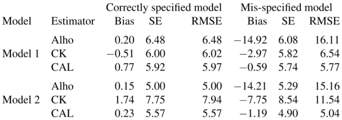
Table 2.1. Performance of three estimators whenn = 600, T = 2. The biases, standard errors, and root mean squared errors are multiplied by100.
Correctly specified model Mis-specified model
Model Estimator Bias SE RMSE Bias SE RMSE
Alho 0.20 6.48 6.48 −14.92 6.08 16.11 Model 1 CK −0.51 6.00 6.02 −2.97 5.82 6.54 CAL 0.77 5.92 5.97 −0.59 5.74 5.77 Alho 0.15 5.00 5.00 −14.21 5.29 15.16 Model 2 CK 1.74 7.75 7.94 −7.75 8.54 11.54 CAL 0.23 5.57 5.57 −1.19 4.90 5.04
CAL, the proposed calibration estimator; CK, Chang and Kott’s estimator; RMSE, root mean squared error; SE, standard error.
yi = 0.4xi+ 0.6x2i +ei, where ei ∼ N(0,1/2). The population correlation betweenxandy
are about 0.85 and 0.42 for Model 1 and Model 2, respectively. We assumed one callback to obtain the followup samples and also assumed the following conditional response model
pit≡pr(δit= 1 |xi, yi, δi,t−1 = 0) ={1 + exp(−αt−φyi)}−1, t = 1,2, (2.17)
where(α1, α2, φ) = (−1,0.5,1). Note thatxi is the nonresponse instrumental variable in this
setup because it is conditionally independent of(δi1, δi2)givenyi.
We computed three estimators ofθ =E(Y): Alho’s estimator obtained from (2.7), Chang
and Kott’s estimator (Chang and Kott , 2008) and the proposed calibration equation estimator obtained by minimizing (2.15). Drew and Fuller (1980) method was not considered in the
simulation because it is applicable only to categorial responses. Chang and Kott’s estimator is ˆ θCK= Pn i=1δiTyi/πˆi Pn i=1δiT/πˆi
where πˆi is obtained by solving
Pn
i=1(δiT/πi−1) (1, xi) = 0with πi = {1 + exp(−α∗ −
φ∗yi)}−1.
Table 2.1 presents the biases, standard errors, and the root mean squared errors of the three estimators under two models with correctly specified response model. All estimators are nearly unbiased except for Chang and Kott’s estimator when the linear relationship betweenyandx
does not hold. Under model 1, both Chang and Kott’s and the proposed calibration equation estimator are more efficient than Alho’s estimator because they directly use the calibration equation, which leads to efficient estimation under a linear relationship. Under Model 2, the linear relationship does not hold and Alho’s estimator is slightly more efficient than the pro-posed estimator because it is based on the maximum likelihood approach. However variance estimation is not easy for Alho’s estimator and, as can be seen in Section 2.5.2, it is not robust against failure of the assumed response model. Chang and Kott’s estimator is very unstable results when the linear relationship betweenyandxdoes not hold. Variance estimation of the calibration equation estimator is computed by (2.16). The relative biases of the variance
esti-mators of calibration equation estimator are less than 5% in both models and are not presented here.
2.5.2 Simulation Two
Under the setup of Simulation One, we considered another type of conditional response model to check the robustness of estimators against mis-specification of this model. In this simulation, we used the distribution as the true response model
pit≡pr(δit= 1 |xi, yi, δi,t−1 = 0) =
Γ(αt+φ)
Γ(αt)Γ(φ)
zαt−1
i (1−zi)φ−1,
where (α1, α2, φ) = (1,0.5,3) and zi = y2i/(1 +y2i). We still used the logistic regression
model (2.17) as the working model for the response mechanism.
Table 2.1 presents the biases, standard errors, and the root mean squared errors of the point estimators under the mis-specified model. Alho’s estimator shows significant biases under both models under the incorrect response model because maximum likelihood estimation is sensitive to departures from the assumed model. Because the proposed calibration equation estimator uses only calibration estimation to estimate the model parameters, the estimated response probability under the incorrect response model still satisfies (2.10) by construction.
Table 2.2 Realized responses in 2009 Korean Local-Area Labor Force survey Status T =1 T =2 T =3 T =4 No response Employment 81,685 46,926 28,124 15,992
Unemployment 1,509 948 597 352 32,350
Not in labor force 57,882 32,308 19,086 10,790
mean squared errors in both models even when the response mechanism is mis-specified.
2.6
Application
In this section, we present an application of the proposed method to the 2009 Korean Local-Area Labor Force Survey. This large-scale labor force survey is designed to get im-proved local-area level estimates. Its samples are a stratified two-stage cluster sample of households in Korea, the primary sampling unit is the segment and the secondary sampling unit is the household. The segments consist of about 30 – 80 households, and are selected with probability-proportional-to-size sampling within each stratum, where the measure of size for the sampling is the number of households based on recent Census information. In the 2009 Korean Local-Area Labor Force Survey data,n= 157,205sample households were contacted with up to four followups. Table 2.2 displays the realized number of respondents for each of the followup attempts.
We assume the conditional response model
pr(δit = 1|δi,t−1 = 0, yi) = {1 + exp(−αt−φyi)}−1, (2.18)
for some(αt, φ), whereyi is the number of unemployed family members in theith household.
We are interested in estimating θ1, θ2 and θ3, which denote the proportion of employment,
unemployment and not in labor force, respectively. Note that θ3 = 1 −θ1 − θ2 and so we
report results forθ1 andθ2 only. Under the assumed response model (2.18), we obtained four
Table 2.3. Estimates for labor force in 2009 Korean Local-Area Labor Force survey
θ1 θ2
Method Estimates(×102) Standard error(×104) Estimates(×102) Standard error(×104)
Naive 58.31 11.05 1.15 2.00
Alho 58.30 10.94 1.19 2.56
Drew & Fuller 58.47 10.90 1.19 2.46
Calibration 58.35 11.05 1.19 2.32
respondents without making any adjustment. The other estimates are computed using Alho (1990)’s method, Drew and Fuller (1980)’s method and our proposed method. Alho’s method uses the model in (2.18). In computing Alho’s method, we use the conditional probability
model (2.18).
Table 2.3 presents the estimates. In Table 2.3, the three more sophisticated methods pro-duce slightly larger estimates for the unemployment rate than the naive method, which implies that the missing rate is higher for unemployed people. Since we do not have any an auxiliary variable that is available throughout the sample in this survey, the three methods show similar results.
Acknowledgement
We thank Dr. Seo-young Kim, two referees, the associate Editor, and editor for construc-tive comments. The research of the first author was supported by a Cooperaconstruc-tive Agreement between the U.S. Department of Agriculture Natural Resources Conservation Service and Iowa State University. The research of the second author was partially supported by Korea National Research Foundation for a study of statistical inference for nonlinear long-memory time series data.
Appendix
Computation for generalized method of moments
To discuss the generalized method of moments computation in Section 2.4, suppose for simplicity that p = 1 andq = 1such that the conditional response probability will be pit =
g(xi, yi;αt, φ1, φ2)fort = 1, . . . , T. Let X = PNi=1xi andY = PiN=1yi. Writingθˆt(x) =
P
i∈Adi{δi,t−1+ (1−δi,t−1)δit/pit}xi, the calibration equation can be expressed as
ˆ θt(1),θˆt(x),θˆt(y) = (N, X, Y) (t= 1, . . . , T), θˆHT(1),θˆHT(x) = (N, X).
Thus, writingθ = (α1,· · · , αT, φ1, φ2), we have estimating formation
U(θ, Y) = X
i∈A
di{ui(1), ui(xi), ui(yi)}T,
where ui(zi) = {ui1(zi), . . . , uiT(zi)} with uit(zi) = {δi,t−1+ (1−δi,t−1)δit/pit(θ)−1}zi
forzi = 1orzi =xi anduit(zi) = {δi,t−1+ (1−δi,t−1)δit/pit(θ)}zi −n−1Y /di forzi = yi
(t= 1, . . . , T).
Writingη = (θ, Y), the covariance matrix ofU(η)is easily computed for a fixed value of ηby ignoring the randomness ofδs. The optimal value ofηcan be obtained by minimizingQ with respect toη
Q=U(η)TV (U)−1U(η). (2.19) We now discuss how to compute the covariance matrixV(U)in (2.19). Let an design-unbiased
estimator of θˆHT(y) = P i∈Adiyi be of the formVˆ = P i∈A P j∈A∆ijyiyj. To estimate the
variance estimator of θˆt(x) = Pi∈Adiηit, where ηit = δit + (1−δi,t−1)δitxi/pit, the naive
variance estimator ˆ Vnaive,t = X i∈A X j∈A ∆ijηitηjt
can be constructed, where∆ij = (πij −πiπj)/(πijπiπj). To see its unbiasedness, note that EVˆnaive,t = E ( X i∈A X j∈A ∆ijE(ηitηjt |At−1) ) = E ( X i∈A X j∈A ∆ijE(ηit|At−1)E(ηjt |At−1) ) +E ( X i∈A X j∈A ∆ijcov(ηit, ηjt |At−1) ) = E X i∈A X j∈A ∆ijxixj ! +E ( X i∈A ∆iivar(ηit|At−1) ) = var X i∈A dixi ! +E ( X i∈A 1−πi π2 i (1−δi,t−1)(p−it1−1)x 2 i ) .
On the other hand,
varnθˆt(x) o = varhEnθˆt(x)|At−1 oi +Ehvarnθˆt(x)|At−1 oi = var X i∈A dixi ! +E ( X i∈A πi−2(1−δi,t−1) (p−it1−1)x 2 i ) .
3 CORRELATION ESTIMATION WITH SINGLY TRUNCATED
VARIABLES
Submitted inStatistical Methods in Medical Research
Jongho Im1, Eunyong Ahn2, Namseon Beck3, Jae-Kwang Kim1and Taesung Park4
Abstract
Correlation coefficient estimates are often attenuated for truncated samples. Motivated from a real data in South Sudan, we consider correlation coefficient estimation in a singly truncated bivariate data. By considering a linear regression model where a truncated variable is used as an explanatory variable, a consistent estimate for the slope can be obtained from the ordinary regression method. A consistent estimator of correlation coefficient is then obtained by multiplying the regression slope coefficient with the variance ratio of the two variables. Two simulation studies were conducted to check the performance of the proposed correlation estimator. The simulation study shows that the proposed estimator is nearly unbiased even un-der non-normal error distributions. The proposed method is applied to South Sudan children’s anthropometric and nutritional data collected by the World Vision.
Key words: A Pearson’s correlation coefficient, outcome dependent sampling, selection bias, truncated regression.
1Department of Statistics, Iowa State University, Ames, U.S.A.
2Interdisciplinary Program in Bioinformatics, Seoul National University, Seoul, South Korea 3International Department, Medair, Echublens, Switzerland
3.1
Introduction
A singly truncated bivariate data are often collected in public health data. For example, we consider in this paper mid-upper arm circumference (MUAC) and weight-for-height Z-score (WHZ) which are often used to determine malnutrition status of infants or young chil-dren. In many cases, children are firstly selected based on MUAC criterion and then WHZ is also measured in the following examinations. On the basis of this process, we have bivariate data (MUAC, WHZ) when MUAC is right truncated and WHZ is not truncated but associated with MUAC. Considering that MUAC is more easily measured than WHZ in the field study at Africa, we are interested in finding how much truncated MUAC is correlated with WHZ. How-ever, the naive approach of computing the sample correlation coefficient estimate is generally biased in a singly truncated data.
One possible way to get an unbiased estimate is to use the maximum likelihood estimator or moment-based estimator under the bivariate normality assumption. In case of singly truncated bivariate data, Aitkin (1964) and Arnold, Beaver and Meeker (1993) proposed a correlation estimator by assuming a bivariate normal distribution. Early works of Cohen (1955), Rosen-baum (1961) and Rao, Garg and Li (1968) were also limited to a bivariate normal distribution. Arismendi (2013) intensively studied the calculation of truncated moments with a multivariate normal distribution.
Here we use a linear regression model rather than the bivariate normal distribution for cor-relation estimation. To consider more general bivariate structures, we decompose the joint probability of two variables as the product of the conditional distribution and the marginal distribution. The conditional distribution is assumed to be a normal linear regression model and the marginal distribution is not necessary to be normal. The linear regression model is constructed so that the singly truncated variable is used as the explanatory variable in the regression model. Then, the regression coefficients are consistently estimated even if the ex-planatory variable is truncated. This desirable result provides an unbiased Pearson’s correlation
coefficient estimator by incorporating variance ratio of the two variables.
In Section 3.2, the basic setup is introduced with model assumptions. In Section 3.3, a correlation estimator is proposed in terms of the product of slope coefficient and variance ratio of variables. Results from a simulation study are presented in Section 3.4 and an application of proposed method to South Sudan children’s anthropometric and nutrition data is conducted in Section 3.5. Concluding remarks are made in Section 3.6.
3.2
Basic setup
Suppose that we have a sample of two random variables(x, y), wherexis right truncated, xi ≤ xc, with knownxc, in the sampling procedure. The truncated sample can be understood
as a sample from two-phase sampling, where the first-phase sample is a random sample and the second-phase sample is a outcome-dependent sample in the sense that the cases withxi > xc
is not selected in the second-phase sampling. Letδi be the sampling indicator for the
second-phase sampling where δi = 1 represents the case when the sample is included in the final
sample andδi = 0otherwise. Outcome-dependent sampling in the context of two-phase
sam-pling is very popular in epidemiology. For example, see Breslow and Cain (1988), Kalbfleisch and Lawless (1988), Wild (1991) and Breslow and Holubkov (1997). Unlike the classical two-phase sampling, we do not have the first-two-phase sample and only have the second-two-phase sample available for analysis.
If our goal is to estimate the regression parameters in the regression ofyonx, we have only to use the final sample for regression analysis without worrying about the sampling procedure. To see this, note that
f(y|x, δ = 1) =f(y|x)R P(δ= 1 |x, y)
P(δ = 1|x, y)f(y|x)dY . (3.1) If the sampling mechanism is a function ofx, then P(δ = 1 |x, y) =P(δ = 1 |x)and (3.1) reduces to
Thus, we can safely ignore the sampling mechanism and apply the standard regression tech-niques to the final data. That is, in estimating the regression parameters, the sampling mecha-nism is non-informative in the sense of Skinner (1994) and Pfeffermann and Sverchkov (1999). However, for estimating the correlation coefficient, the sampling mechanism becomes infor-mative becausef(x, y | δ = 1) 6= f(x, y). Thus, we cannot directly use the standard method to estimate the correlation coefficient.
Early works of correlation estimation with singly truncated data were mostly based on bivariate normal assumption. Aitkin (1964) provided correlation estimator in terms of Mill’s ratio, ˆ ρ= p rR(xc) R(xc)2+ (1−r2)(xcR(xc)−1) , whereR(xc) = exp(x2c/2) Rxc −∞exp(−t
2/2)dt is Mill’s ratio andris a sample correlation
co-efficient of truncated samples. His work is limited to the standard bivariate normal distribution. Arnold, Beaver and Meeker (1993) extended Aitkin (1964)’s work to a general bivariate normal distribution with mean vector(µx, µy), variance vector(σ2x, σ2y)and correlationρ. From
the truncated variablex, they derived the distribution ofyin terms of skew normal distribution. They expressed three moments of untruncated variable y of E(y), var(y) and Skewness(y) with three unknown parameters, µy, σy2 and ρ, and then obtained the method of moments
estimates for the unknown parameters by solving three moment equations. Also they provided likelihood function ofyincluding the skewness parameter (Cartinhour, 1990) which is a non-linear function ofρ. Thus, they also computed the maximum likelihood estimator of ρusing the proposed likelihood function. However, their approach is limited to the specific case, in which a truncated point ofxisE(x).
3.3
Proposed method
We now consider a new approach of parameter estimation of bivariate data (x, y) when the sample is observed with truncated x. We use a marginal distribution and a conditional
distribution to get the joint probability function for(x, y) such thatf(y, x) = f(y | x)f(x). Sincef(y | x, δ = 1) = f(y | x), the parameters in the conditional distribution is easy to be obtained. The marginal distribution ofxis assumed to be parametrically specified withf(x;γ). Parameter γ is obtained by maximizing the observed likelihood that reflects the truncation mechanism.
We assume that the conditional distribution takes the form of a classical linear regression model, given by
y = β0+β1x+e, e∼(0, σe2), (3.3)
whereeis uncorrelated withx.
SinceE(ei | xi, δi = 1) =E(ei |xi) = 0by (3.2), the consistent estimates of( ˆβ0,βˆ1,σˆe2)
can be obtained by the ordinary least squares method. That is, the normality on the error distribution is not needed.
Now, we first consider the case whenxis normally distributed withN(µx, σx2). To estimate
the marginal parameter(µx, σ2x), note that
f(x|δ = 1) =f(x|x < xc) =
φ{(xc−µx)/σx}I(x < xc) {Φ(xc−µx)/σx}
,
whereφis the probability density function andΦ(x) =R−∞x φ(z)dz is the cumulative density function of standard normal distribution, respectively. The observed log-likelihood is
l2(µx, σx2) = − 1 2nlogσ 2 x− 1 2σ2 x X i (xi−µx)2− X i log Φ xc−µx σx . (3.4) Note that the maximum likelihood estimators for (3.4) are the solutions of non-linear equations
which are derivatives ofl2(µx, σx2)with respect to(µx, σ2x). One can also use an EM algorithm
to obtain the MLE (Kim and Shao, 2013).
We now consider the case when xis not normally distributed. Ifxis parametrically spec-ified with a density function f(x;γ) with an unknown parameter γ, then the observed log-likelihood function is l2(γ) = X i logf(xi;γ)− X i logF(xc;γ), (3.5)
whereF(x) = R−∞x f(x)dx is a cumulative density function ofx. The maximum likelihood estimator ofγcan be obtained by maximizing (3.5).
Once we assume a parametric distribution on truncated x, we can make a goodness-of-fit test to reduce mis-specification risks. For the truncated or censored sample version of Kolmogorov-Smirnov goodness-of-fit tests were studied in various ways such as Barr and Davidson (1973), Koziol and Byar (1975), Dufour and Maag (1978) and Fleming et. al. (1980). Here, we consider modified Kolmogorov-Smirnov test assuming the conditional distribution of truncatedxwith an unknown parameterγ,
Dn= sup
−∞≤x≤xc
|Fˆn(x)−F0(x;γ)|, (3.6)
where Fˆn(x) is a empirical cumulative density function with Fˆn(x) = 1n
P
iI(xi ≤ x) and
F0(x;γ)is the cumulative distribution function of truncatedxwhich is defined by
F0(x;γ) = Z x −∞ f(t;γ) F(xc;γ) dt.
Since γ is an unknown parameter, we can use estimated parameters for goodness-of-fit test. Given the estimated parameters, we have a modified test statistic,
Dn(ˆγ) = √ n max x(i),...,x(n) | i n −F0(x(i); ˆγ)|, (3.7) wherexkis thekth largest value amongx1, . . . , xn.
Durbin (1975) showed how the modified Kolmogorov-Smirnov test works when parame-ters are estimated. When the same Kolmogoronov distribution is used to the compute p-value, using the estimated parameters gives more unstable results to specify the distribution of X rather than using true parameters. In practice, one can first consider a normal distribution and perform a goodness-of-fit test. If the test result shows a significant departure from normality, we may consider an alternative model.
We now want to estimate Pearson’s correlation coefficient defined by
ρxy =corr(x, y) =cov(x, y)/
p
Since the regression slope coefficientβ1 can be expressed with cov(x, y)and var(x)under the
linear regression,
β1 =cov(x, y)/var(x),
the Pearson’s correlation coefficient can be driven in terms ofβ1, var(x)and var(y)withρ =
β1
p
var(x)/pvar(y).Thus, the proposed estimator ofρwould be ˆ
ρ= ˆβ1
p ˆ
var(x)/pvar(ˆ y), (3.8) whereβˆ1 is the maximum likelihood estimator obtained by maximizing of the log-likelihood
function of normal distribution andvar(ˆ x)and var(ˆ y) are respectively obtained from the as-sumed distribution ofxandygivenx. Since the variance ofxcould be defined as a function of assumed distribution parameters in general, we can computevar(ˆ x)using those parameter estimates. Also, we can compute var(ˆ y) with the law of total variance, var(y) = E[var(y |
x)] +var[E(y | x)]. For example, we get var(y) = σ2
e +β12var(x)in the linear regression
model (3.3).
Remark 1 Instead of assuming a marginal distribution of x, we may assume a conditional distribution ofxgivenysuch as another simple linear regression ofxonysuch that
x=α0 +α1y+u, u∼N(0, σu2). (3.9)
Then, another unbiased estimatorρˆis
ˆ
ρ= ˆα1βˆ1, (3.10)
whereαˆ1is obtained by maximizing the following conditional log-likelihood function:
lc(α, σ2u) = − 1 2nlogσ 2 u− 1 2σ2 u X i (xi−α0−α1yi)2 −X i log Φ xc−α0−α1yi σu . (3.11)
Even if the log-likelihood (3.11) is not globally concave, it has a unique maximum in the interior of parameter space, if one exist (Orme, 1989). Truncated regression has been largely
studied in economics. For example, see Amemiya (1973), Olsen (1980), Goldberger (1981) and Green (1983).
We now discuss variance estimation of the coefficient estimator in (3.8). Note that we can
express that ˆ ρ= ˆβ1 ˆ σx2 ˆ σ2 e + ˆβ21σˆ2x !1/2 (3.12) and the three estimators,βˆ1,σˆe2, andσˆ2x, are mutually uncorrelated. We can apply Taylor
lin-earization to obtain linlin-earization variance formula. The closed-form estimates for the variance ofρˆin (3.12) is ˆ V( ˆρ) = A2var( ˆˆ β1) +B2var(ˆˆ σx2) +C 2var(ˆˆ σ2 e), (3.13) where A = ˆ σ2x ˆ σ2 y 1/2 1− σˆ 2 x ˆ σ2 y ˆ β12 , B = ˆ β1 2ˆσ2 y σˆ2 y ˆ σ2 x 1/2 1− σˆ 2 x ˆ σ2 y ˆ β12 , C = − βˆ1 2ˆσ2 y ˆ σ2 x ˆ σ2 y 1/2 , andσˆ2
y = ˆσ2e + ˆβ12ˆσ2x. The variance estimates of
n ˆ
var( ˆβ1),var(ˆˆ σe2)
o
can be directly computed from the inverse of expected Fisher information or observed Fisher information with estimated parameters. Furthermore, the variance estimate var(ˆˆ σ2
x) can be also estimated through the
negative Hessian matrix of (3.4) or Taylor linearization based on variance estimates of var(ˆγ)
in (3.5). For the bivariate normal distribution example, we have
ˆ var( ˆβ1) = ˆ σ2 e P i(xi−x¯)2 , ˆ var(ˆσe2) = n 2ˆσ4 e − P i(yi−βˆ0−βˆ1xi)2 ˆ σ6 e !−1 , and{var(ˆˆ µx),var(ˆˆ σx2)}are approximated by the diagonal ofI(ˆµx,σˆx2)−1,
I(µx, σx2) =− I11(µx, σx2) I12(µx, σx2) I12(µx, σx2) I22(µx, σx2) ,
where I11 = − n ˆ σ2 x +n ( (xc−µˆx) ˆfFˆ ˆ σ2 x + ˆf2 ) /Fˆ2, I12 = − P i(xi−µˆx) ˆ σ4 x +n (xc−µˆx)2 2ˆσ4 x − 1 2ˆσ2 x ˆ fFˆ+ (xc−µˆx) 2ˆσ2 x ˆ f2 /Fˆ2, I22 = n 2ˆσ4 x − P i(xi−µˆx)2 ˆ σ6 x −n 3(xc−µˆx) 4ˆσ4 x −(xc−µˆx) 3 4ˆσ6 x ˆ fFˆ− (xc−µˆx) 2 4ˆσ4 x ˆ f2 /Fˆ2, withfˆ= (2πσˆx2)−1/2exp{−(xc−µˆx)2/2ˆσ2x}andFˆ =
Rxc
−∞(2πσˆ
2
x)−1/2exp{−(t−µˆx)2/2ˆσ2x}dt.
3.4
Simulation Study
We conducted two simulation studies to check the performance of the proposed method. In the first simulation, we generated bivariate samples(x, y)with sizenas the first-phase sample and then dropped sub-samples which correspond toxi >1. We used two levels ofn:n = 400
andn = 800. In the first simulation, the classical linear regression ofyonxis assumed:
yi =β0+β1xi +ei,
where ei ∼ N(0,0.5) with (β0, β1) = (1,1) and xi are generated from normal distribution
N(1,1)or gamma distribution Gamma(1,1).
For the second simulation, given the normality of x, we considered non-normal distribu-tions ofygivenxsuch thatefollows a t-distribution or a gamma distribution. Through those simulation studies, we checked how our proposed estimator is robust to mis-specification of regression model assuming normality.
We generated 2,000 Monte Carlo samples for each simulation study and computed three estimators ofρ:
1. ρˆnaive: a naive estimator which is the standard sample correlation estimator with
trun-cated samples, ˆ ρnaive = P i(xi−x¯)(yi−y¯) pP i(xi−x¯)2 P i(yi−y¯)2 .
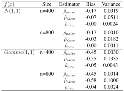
Table 3.1 Monte Carlo Mean bias and variance of( ˆρ)under simulation one f(x) Size Estimator Bias Variance
N(1,1) n=400 ρˆnaive -0.17 0.0019 ˆ ρskew -0.07 0.0511 ˆ ρnew -0.00 0.0024 n=800 ρˆnaive -0.17 0.0010 ˆ ρskew -0.03 0.0182 ˆ ρnew -0.00 0.0011 Gamma(1,1) n=400 ρˆnaive -0.45 0.0030 ˆ ρskew -0.55 0.1335 ˆ ρnew -0.05 0.0043 n=800 ρˆnaive -0.45 0.0014 ˆ ρskew -0.58 0.1000 ˆ ρnew -0.04 0.0024
2. ρˆskew: a maximum likelihood estimate ofρobtained by maximizing the likelihood
func-tion of the skew normal distribufunc-tion (Arnold, Beaver & Meeker, 1993),
L(µy, σy, ρ) = Y i 2 σy φ y−µy σy Φ −λy−µy σy ,
whereλ =ρ(1−ρ2)−1/2. See Azzalini (1985) for details of the skew normal distribution. 3. ρˆnew: an estimate obtained using the proposed estimator (3.8).
Note that if a truncation point is not equal to the expected value ofx, then we have an identifi-cation problem in estimation ofρˆskew. See Arnold, Beaver & Meeker (1993) for details.
Table 3.1presents the Monte Carlo biases and variances of the three estimators under the
first simulation and the result of Table 1 shows that our proposed estimator provides nearly unbiased estimates when the marginal distribution of x is correctly specified. The standard sample correlation estimates seriously underestimate the true correlation for both truncated samples. The maximum likelihood estimates of the skew normal distribution are relatively unbiased for the normal case but they are seriously biased for the non-normal cases. Since the correlationρis a function of skewness parameterλin the skew normal distribution, its estimate
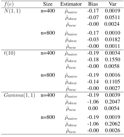
Table 3.2 Monte Carlo Mean bias and variance of( ˆρ)under simulation two f(e) Size Estimator Bias Var
N(1,1) n=400 ρˆnaive -0.17 0.0019 ˆ ρskew -0.07 0.0511 ˆ ρnew -0.00 0.0024 n=800 ρˆnaive -0.17 0.0010 ˆ ρskew -0.03 0.0182 ˆ ρnew -0.00 0.0011 t(10) n=400 ρˆnaive -0.19 0.0034 ˆ ρskew -0.18 0.1550 ˆ ρnew -0.00 0.0058 n=800 ρˆnaive -0.19 0.0016 ˆ ρskew -0.14 0.1105 ˆ ρnew -0.00 0.0027 Gamma(1,1) n=400 ρˆnaive -0.19 0.0039 ˆ ρskew -1.06 0.2047 ˆ ρnew 0.00 0.0054 n=800 ρˆnaive -0.19 0.0019 ˆ ρskew -1.06 0.2062 ˆ ρnew -0.00 0.0026
severely depends on the skewness of truncated samples and this makes the estimates of true correlation very unstable. Also, for variance estimation, the absolute value of relative biases of Vˆ( ˆρnew) in (3.13) are less than 3% in all cases which shows that the proposed variance
estimator is nearly unbiased. The results are not presented here for brevity.
Table 3.2presents the Monte Carlo biases and variances of the three estimators under the
second simulation. Table 3.2 shows that our proposed estimator assuming the normal error
also works well under non-normal error distribution in the linear regression of y on x. For a large sample size(n = 800), the regression slope estimates and its inference are robust to departures from the normal error assumption. That is, we can obtain nearly unbiased estimates ofβ1 and var(y | x)by constructing of a regression with truncated covariate and untruncated
dependent variable for bivariate singly truncated samples. This desirable robustness makes the proposed estimator (3.8) consistent under various model scenarios.
3.5
Application
From 2006 to 2013, the ‘World Vision’ collected the anthropometric and nutritional data from Community-based Management of Acute Malnutrition in South Sudan. Initially these data are recorded as handwriting on the paper sheets, but they are entered into 15 Excel files by the data entering staffs in World Vision East Africa Regional Office. The aim of Community-based Management of Acute Malnutrition program is to reduce the infant or child death due to famine and the procedure of the program is as following. At first, the nutritional status of chil-dren aged less than 5 are screened by measuring the mid-upper arm circumference(MUAC). If the children falls on the criteria of severe acute malnutrition, then they were referred to the community treatment center for treatment. Whenever children visited the nutrition center, the full anthropometric measurements were reassessed and recorded on the patients sheet by the health workers with the treatment center. World Vision South Sudan collected the recorded sheets for years and we were asked to analyze the data statistically to evaluate the current pro-cedures and criteria. The quality control process of the collected data resulted in total 3,488 sets of patients data, but some of them are still subject to missingness in basic anthropometric variables.
The World Health Organization (WHO) and the United Nations Children’s Fund (UNICEF) recommend to use a criteria to determine malnutrition: either mid-upper arm circumference (MUAC)<115mm or weight-for-height Z-score (WHZ)<-3. However, MUAC is mostly used to identify the malnourished children who should be included in the malnutrition program, because it is challenging to measure the height and weight together with MUAC. Thus, this leads to generation of singly bivariate observations for MUAC measurement from the field operation.
In case of the World Vision data, children whose MUAC are larger than 115mm are also non-randomly selected to be enrolled in the malnutrition program as measurement errors by the community workers. Thus, we choose children whose MUAC is less than 115mm and
● ● ● ● ● ● ● ● ● ● ● ● ● ● ● ● ● ● ● ● ● ● ● ● ● ● ● ● ● ● ● ● ● ● ● ● ● ● ● ● ● ● ● ● ● ● ● ● ●● ● ● ● ● ● ● ● ● ● ● ● ● ● ● ● ●● ● ● ● ● ● ● ● ● ● ● ● ● ● ● ● ● ● ● ● ● ● ● ● ● ● ● ● ● ● ● ● ● ● ● ● ● ● ● ● ● ● ● ● ● ● ● ● ● ●● ● ● ● ● ● ● ● ● ● ● ● ● ● ● ● ● ● ● ● ● ● ● ● ● ● ● ● ● ● ● ● ● ● ● ● ● ● ● ● ● ● ● ● ● ● ● ● ● ● ● ● ● ● ● ● ● ● ● ● ● ● ● ● ● ● ● ● ● ● ● ● ● ● ● ● ●● ● ● ● ● ● ● ● ● ● ● ● ● ● ● ● ● ● ● ● ● ● ● ● ● ● ● ● ● ● ● ● ● ● ● ● ● ● ● ● ● ● ● ● ● ● ● ● ● ● ● ● ● ● ● ● ● ● ● ● ● ● ● ● ● ● ● ● ● ● ● ● ● ● ● ● ● ● ● ● ● ● ● ● ● ● ● ● ● ● ● ● ● ● ● ● ● ● ● ● ● ● ● ● ● ● ● ● ● ● ● ● ● ● ● ● ● ● ● ● ● ● ● ● ● ● ● ● ● ● ● ● ● ● ● ● ● ● ● ● ● ● ● ● ● ● ● ● ● ● ● ● ● ● ● ● ● ● ● ● ● ● ● ● ● ● ● ● ● ● ● ● ● ● ● ● ● ● ● ● ● ● ● ● ● ● ● ● ● ● ● ● ● ● ● ● ● ● ● ● ● ● ● ● ● ● ● ● ● ● ● ● ● ● ● ● ● ● ● ● ● ● ● ● ● ● ● ● ● ● ● ● ● ● ● ● ● ● ● ● ● ● ● ● ● ● ● ● ● ● ● ● ● ● ● ● ● ● ● ● ● ● ● ● ● ● ● ● ● ● ● ● ● ● ● ● ● ● ● ● ● ● ● ● ● ● ● ● ● ● ● ● ● ● ● ● ● ● ● ● ● ● ● ● ● ● ● ● ● ● ● ● ● ● ● ● ● ● ● ● ● ● ● ● ● ● ● ● ● ● ● ● ● ● ● ● ● ●● ● ● ● ● ● ● ● ● ● ● ● ● ● ● ● ● ● ● ● ● ● ● ● ● ● ● ● ● ● ● ● ● ● ● ● ● ● ● ● ● ● ● ● ● ● ● ● ● ● ● ● ● ● ● ● ● ● ● ● ● ● ● ● ● ● ● ● ● ● ● ● ● ● ● ● ● ● ● ● ● ● ● ● ● ● ● ● ● ● ● ● ● ● ● ● ● ● ● ● ● ● ● ● ● ● ● ● ● ● ● ● ● ● ● ● ● ● ● ● ● ● ● ● ● ● ● ● ● ● ● ● ● ● ● ● ● ● ● ● ● ● ● ● ● ● ● ● ● ● ● ● ● ● ● ● ● ● ● ● ● ● ● ● ● ● ● ● ● ● ● ● ● ● ● ● ● ● ● ● ● ● ● ● ● ● ● ● ● ● ● ● ● ● ● ● ● ● ● ● ● ● ●● ● ● ● ● ● ● ● ● ● ● ● ● ● ● ● ● ● ● ● ● ● ● ● ● ● ● ● ● ● ● ● ● ● ● ● ● ● ● ● ● ● ● ● ● ● ● ● ● ● ● ● ● ● ● ● ● ● ● ● ● ● ● ● ● ● ● ● ● ● ● ● ● ● ● ● ● ● ● ● ● ● ● ● ● ● ● ● ● ● ● ● ● ● ● ● ● ● ● ● ● ● ● ● ● ● ● ● ● ● ● ● ● ● ● ● ● ● ● ● ● ● ● ● ● ● ● ● ● ● ● ● ● ● ● ● ● ● ● ● ● ● ● ● ● ● ● ● ● ● ● ● ● ● ● ● ● ● ● ● ● ● ● ● ● ● ● ● ● ● ● ● ● ● ● ● ● ● ● ● ● ● ● ● ● ● ● ● ● ● ● ● ● ● ● ● ● ● ● ● ● ● ● ● ● ● ● ● ● ● ● ● ● ● ● ● ● ● ● ● ● ● ● ● ● ● ● ● ● ● ● ● ● ● ● ● ● ● ● ● ● ● ● ● ● ● ● ● ● ● ● ● ● ● ● ● ● ● ● ● ● ● ● ● ●● ● ● ● ● ● ● ● ● ● ● ● ● ● ● ● ● ● ● ● ● ● ● ● ● ● ● ● ● ● ● ● ● ● ● ● ● ● ● ● ● ● ● ● ● ● ● ● ● ● ● ● ● ● ● ● ● ● ● ● ● ● ● ● ● ● ● ● ● ● ● ● ● ● ● ● ● ● ● ● ● ● ● ● ● ● ● ● ● ● ● ● ● ● ● ● ● ● ● ● ● ● ● ● ● ● ● ● ● ● ● ● ● ● ● ● 80 90 100 110 −6 −4 −2 0 2 MUAC WHZ
Figure 3.1 Scatter plot with regression line 1,115 cases are refined with both observed MUAC and WHZ.
Since the bivariate samples are singly truncated by MUAC, we firstly assume a linear re-gression of WHZ on MUAC,
WHZ=β0+β1MUAC+e, (3.14)
wheree∼N(0,1)and MUAC are assumed to be originally generated from truncated normal distribution.
The correlation coefficient estimate is computed by the following four steps: (Step 1) Estimate the parameters in the specified model.
(Step 2) Conduct a goodness-of-fit test on MUAC with estimated parameters.
(Step 3) Estimate regression slope coefficientβ1in (3.14) using the ordinary least squares method.
Table 3.3 Counts for observed and expected MUAC <105 105∼115
Observed 277 838 Expected 290 825
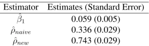
Table 3.4 Regression analysis: MUAC and WHZ Estimator Estimates (Standard Error)
ˆ β1 0.059 (0.005) ˆ ρnaive 0.336 (0.029) ˆ ρnew 0.743 (0.029)
Since MUAC has many ties at specific points as shown in Figure3.1, we used the Pearson’s
chi-squared test instead of the Kolmogorov-Smirnov test. To reduce heaping effect, MUAC is categorized into two bins based on 105 and then we computed observed cases and expected cases. The expected number is calculated using the cumulative density function of conditional distribution with estimated parameters,µˆM U AC = 161andσˆM U AC2 = 426,
n Z c2 −∞ f(x; ˆµx,ˆσx2)dx− Z c1 −∞ f(x; ˆµx,σˆx2)dx / Z 115 −∞ f(x; ˆµx,σˆx2)dx,
wherex represents MUAC, c1 andc2 are determined from (−∞,105,115), andn = 1,115.
Also the expected number is cumulatively rounded to have integer value. We get the chi-squared test statistic (0.79) and p-value (0.37) from the numbers in Table 3.3. This implies
that normal assumption on MUAC is acceptable and it allows us to safely compute correlation coefficient estimate.
Correlation estimation results are summarized in Table3.4. The proposed method produces
a higher correlation coefficient estimate comparing to the naive sample correlation coefficient estimate. The standard error of proposed estimator is calculated using the linearization formula in (3.13).
3.6
Conclusion
Motivated from real data collected by the World Vision, we have considered the Pearson’s correction coefficient estimator for a singly truncated bivariate data. A regression model and parametric marginal distribution are assumed instead of bivariate normal distribution on two variables.
In the parametric model for the marginal distribution, one may consider a candidate distri-bution such as normal distridistri-bution and then use a modified Kolmogorov-Smirnov test to test for goodness-of-fit. Once the specified model is accepted, its parameters can be estimated by maximizing the conditional likelihood described in (3.5). For the regression of untruncated
variable on truncated variable, we assume a classical linear regression model which allows for non-normal error distributions.
Once we compute the variance of truncated variable and the slope coefficient in the regres-sion model, we can estimate the Pearson’s correction coefficient using the simple formula in (3.12). Our simulation study showed that the proposed estimator works well for non-normal
truncated variable and also works when the error distribution of linear regression model is no longer normal.
The proposed method is applied to the real malnutrition data collected by World Vision of Africa which measure two malnutrition indicators, WHZ and MUAC. With truncated data, the correlation between two measurements is usually attenuated. The proposed method is applied to the truncated data and the result shows much higher correlation between the two measurements.
4 TWO-PHASE STRATIFIED SAMPLING FOR FRACTIONAL HOT
DECK IMPUTATION
Jongho Im1, Jae kwang Kim1and Wayne A. Fuller1
Abstract
Hot deck imputation is popular in handling item nonresponse in survey sampling. In hot deck imputation, imputed values are taken from the respondents in the same imputation cell. Imputation cells are used to approximate the imputation model nonparametrically. We extend the fractional hot deck imputation of Kim and Fuller (2004) to the case when some part of imputation cells are also missing. The proposed method of fractional hot deck imputation is performed in two steps and has a similar structure of two-phase stratified sampling. The proposed hot deck imputation method is directly applicable to multivariate missing data with different missing patterns. For variance estimation, we use replication based approach with additional replicates to account for the additional imputation variance. Some numeral results from two simulation studies are also presented.
Key words: Cell mean model; Item nonresponse; EM algorithm, Multivariate missing; Replication variance estimation.
4.1
Introduction
Nonresponse is frequently encountered in survey sampling. Unit nonresponse and item nonresponse are two major types of nonresponse (Kalton and Kasprzyk,1986). While
ing adjustment is commonly used to compensate for unit nonresponse, imputation is preferred to handle item nonresponse. Several different imputation methods have been introduced in the literature. Examples of imputation methods include mean imputation, regression imputation, hot deck imputation and nearest neighbor imputation, and so forth. Hazziza (2009) provides a comprehensive overview of those imputation methods.
In household surveys, hot deck imputation is a very popular imputation method. In hot deck imputation, the imputed values are the real observations taken from the respondents in the same sample. Hot deck imputation is popular because it does not create artificial values and also it does not rely on strong model assumptions unlike the imputation method using parametric models. In hot deck imputation, creating imputation cells to achieve homogeneity within imputation cells is critical. In Brick and Kalton (1996), all auxiliary variables are treated as categorical and imputation cells are formed as a combination of those categorized auxiliary variables. A nearest-neighbor imputation approach uses a metric distance of auxiliary variables that is used to find the set of donors (Cotton, 1991; Rancourt, S¨arndal and Lee, 1994 and Chen and Shao, 2000). Also Hazziza and Beaumont (2007) uses the score estimated by the regression of response on the auxiliary variables or conditional expectation of study variable to create imputation cells.
Variance estimation after hot deck imputation is a challenging problem because it is well known that native approach of treating imputed values as if observed and applying standard variance estimation formula often underestimates the true variance. Rubin (1987) proposed multiple imputation as a general tool for inference with imputed data. In multiple imputation, more than one, say M(> 1), imputed estimates are created for each missing item and then the imputation values are combined using Rubin’s formula for variance estimation. Rubin and Schenker (1986) proposed approximate Bayesian bootstrap (ABB) imputation as a hot deck approach to multiple imputation.
On the other hand, instead of multiple imputation, fractional imputation is also proposed (Kalton and Kish, 1984; Kim and Fuller, 2004) as a way of achieving efficient hot deck
impu-tation. Similarly to multiple imputation, M imputed values are generated in fractional impu-tation, but single data set is created after fractional imputation. Fractional weights are used to handle several imputed values and replication methods are used for variance estimation. Kim and Fuller (2004) and Fuller and Kim (2005) described some properties of fractional hot deck imputation and discussed variance estimation.
In the fractional hot deck imputation of Kim and Fuller (2004), imputation cells are pre-determined and the cell mean model is assumed within imputation cells. The determination of imputation cell is not discussed in the Kim and Fuller (2004). In practice, the imputation cells are chosen to achieve homogeneity within imputation cells but sometimes such assumption is not always easy to verify.
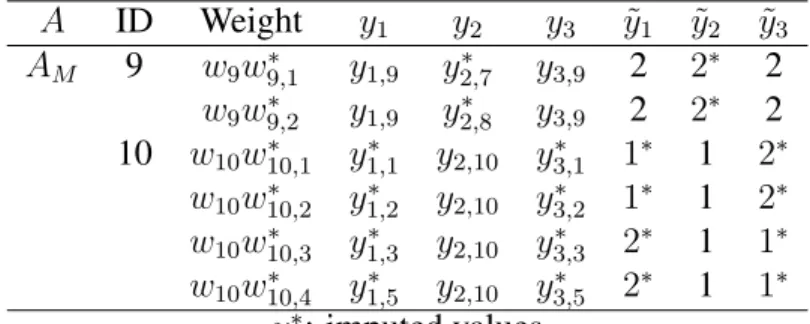
In this paper, we consider an extension of fractional hot deck imputation of Kim and Fuller (2004) in two ways. First, instead of assuming that the imputation cells are given, we allow multiple cells for each missing item to account for full uncertainty associated with cell determi-nation. The procedure can be understood as a nonparametric approximation of the true model by a finite mixture model. The implementation of fractional hot deck imputation under the finite mixture model is made through a two-phase stratified sampling mechanism. Second, the proposed method is applied to multivariate missing data with arbitrary missing patterns, using the proposed two-phase stratification approach to determine the imputation cells and compute fractional weights. The joint distribution of the study items are nonparametrically estimated by using a discrete approximation using imputation cells. The joint probabilities of the cells under missing data are computed from a modified EM algorithm and these estimated joint probabilities are used to determine the weights of imputation cells. The replication jackknife variance estimator is proposed for the variance estimation of imputed estimator.
In Section4.2, the basic setup is introduced. The proposed two-phase stratified fractional
imputation and its variance estimation are discussed for a univariate case in Section 4.3. In
Section4.4, the proposed method is extended to the general case of multivariate missing data.
are made in Section4.6.
4.2
Basic setup
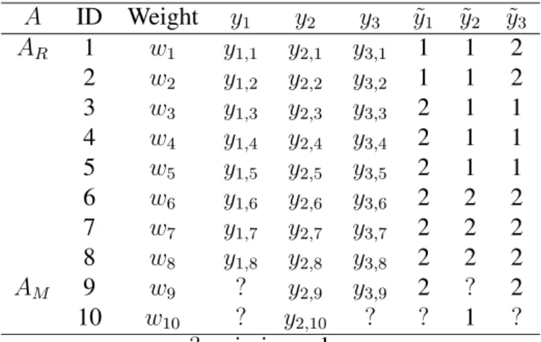
Suppose that we have a finite population of sizeN, indexed byU ={1,2,· · ·, N}, and let Abe the index set for the units in the sample selected by a probability sampling mechanism. LetAbe partitioned intoGgroups based on the auxiliary informationx, wherextakes values on {1,· · · , G}. Thus, we can write A = A1 ∪ · · · ∪ AG. In addition to x, we collect y
andz whereyis the study variable andz is another categorical variable that takes values on
{1,· · · , H}. The cross classification ofxandz forms imputation cell and we assume that yi |(xi =g, zi =h)∼ii(µgh, σ2gh), i∈U, (4.1)
for someµgh andσ2gh > 0, where ∼ iidenotes independently and identically distributed. We
now write zi = (zi1, . . . , ziH)andzih is the indicator function that takes the value one if unit
i ∈ Ag belongs to cell(gh)and is zero otherwise. We assume thatxi is always observed but
(yi, zi)are subject to missingness. Defineδi = 1if(yi, zi)is observed andδi = 0otherwise.
We assume that the response mechanism is missing at random (MAR) in the sense thatδis conditionally independent of(y, z)givenx. That is,
f(y, z |x, δ) =f(y, z |x). (4.2)
Then, from the conditions (4.2), we have
f(y|x, z, δ) = f(y |x, z)f(δ|x)/f(δ|x, z)
= f(y |x, z), (4.3)
where the second equality comes from condition (4.2). Thus, from result (4.3), then model
(4.1) also holds for the responding units. That is,
We now consider a hot deck imputation estimator of YN =
PN
i=1yi under nonresponse.
Since MAR condition (4.2) holds, the following estimator
ˆ YI =
X
i∈A
wi{δiyi+ (1−δi)E(yi |xi, δi = 1)}. (4.5)
is unbiased forYN, wherewi is a sampling weight for uniti.
Now, by the conditions (4.2) and (4.3), we write
f(y|x, δ= 1) = f(y|x) = X z P(z |x)f(y |x, z) = X z P(z |x, δ = 1)f(y|x, z, δ = 1). (4.6)
Model (4.6) takes the form of a finite mixture model. Letπh|g =P(zh = 1 |x=g)be the
conditional probability ofzh = 1givenx=g. Here, the variables(x, z)can be understood as
the imputation cell variables for hot deck imputation. Note that, from (4.6), we have
E(y|x=g) =
H
X
h=1
πh|gE(y|x=g, zh = 1).
To constructE(yi | xi, δi = 1)in (4.5), therefore, we first generatezi∗ fromP(zi | xi, δi = 1)
and then generatey∗i fromf(yi |xi, zi∗).
Thus, if πh|g is known, we can use all the respondents in the cell to estimate E(y | x =
g, zh = 1)to get ¨ YF EF I = G X g=1 X i∈Ag wi ( δiyi+ (1−δi) H X h=1 πh|gy¯Rgh ) , (4.7) where ¯ yRgh = P i∈Agwiδizihyi P i∈Agwiδizih
is the weighted mean of respondents in cell (gh). The imputed estimator of (4.7) uses all
observed values as donors in the imputation cell and this estimator is often called the fully efficient fractional efficient (FEFI) estimator (Kim and Fuller, 2004). Note that FEFI estimator in (4.7) is unbiased forYN =
PN
i=1yi under non-informative sampling design and is